Article

Linear Parameter-Varying Model Predictive Control for Hydraulic Wind Turbine

College of Electrical Engineering and Automation, Shandong University of Science and Technology, Qingdao 266590, China
*
Author to whom correspondence should be addressed.
Actuators 2022, 11(10), 292; https://doi.org/10.3390/act11100292
Submission received: 29 July 2022 / Revised: 29 September 2022 / Accepted: 8 October 2022 / Published: 12 October 2022
(This article belongs to the Special Issue Modern Control in Theory and Practice)

Abstract

:
Wind speed uncertainty and measurement noise affect the control effect in hydraulic wind turbine systems. This paper proposes a model predictive control (MPC) method with a dynamic Kalman filter (KF) based on a linear parameter-varying (LPV) model to address this problem. First of all, the LPV model for a nonlinear system of a hydraulic wind turbine is established using function substitution. Then, a LPV-based KF is introduced into the MPC to provide more precise estimated results and improve the anti-interference ability of the system. According to the current condition of the hydraulic wind turbine, the method updates the Kalman state estimator at each sampling instant and computes the optimal control input by solving a quadratic programming (QP) optimization problem. The performance and the efficiency of the proposed method is validated in simulation and compared with other methods.

1. Introduction

With the increasing tension caused by the global energy demand and the gradual increase in environmental pollution, the development of renewable energy is particularly important. Wind power, as a renewable and clean energy source, has received attention from all over the world. Due to the harsh operating environment of wind turbines and the disturbances caused by environmental factors that are difficult to control in wind power systems, it is necessary to ensure the wind energy conversion efficiency and stable operation of wind farms.
The wind turbine is a relatively complex type of equipment that converts wind energy into electrical energy. According to different transmission systems, wind turbines are divided into traditional gear transmission, gearless direct-drive transmission and hydraulic transmission [1]. Wind speed uncertainty often leads to an increase in gearbox failure rate and high maintenance costs for gear-driven wind turbines [2]. The direct-drive structure of permanent magnet synchronous generators can replace gearboxes. However, rare-earth permanent magnet materials cause the problem of high manufacturing costs of permanent magnet synchronous generators [3]. In addition, a full-power rectifier inverter is required, further increasing the investment cost [4]. In order to overcome the above disadvantages, hydraulic transmission may be a feasible alternative. In the hydraulic wind turbine, hydraulic transmission replaces the gearbox transmission of the traditional wind turbine and transmits the mechanical energy captured by the wind turbine rotor to the generator. In addition, hydraulic transmission can separate the speed of the wind turbine rotor from that of the synchronous generator, and no additional frequency conversion device is required [5,6].
The nonlinearity of hydraulic wind turbines, the uncertainty of the system parameters and the constraints of the system variables are considered important challenges faced by wind turbines in their modeling and control. According to the characteristics of each part of hydraulic wind turbines, the mathematical model of the corresponding part was established to study the dynamic behavior of wind turbines [7,8]. The literature [9] established a nonlinear state space model of a hydraulic wind turbine with two hydraulic pumps, and used it to control the generator speed and track the maximum power point. This literature did not linearize the hydraulic wind turbine model. The nonlinear problem of hydraulic wind turbines was further treated by transforming it into an extended linear form, which was used to design a gain-scheduled linear quadratic regulator (LQR) to achieve the tracking of the desired trajectory [10]. The literature [11,12] used a small-signal linearization method to linearize the hydraulic wind turbine model and analyzed the working area of the power transmission system for the stable adjustment of the transmission power. However, hydraulic wind turbines have nonlinearity and time-varying characteristics due to their own system characteristics and external uncertainties, so the model parameters needed to be adjusted accordingly. Therefore, the LPV was used to model the hydraulic wind turbine. Rugh and Shamm [13] proposed the LPV theory, which introduced variable parameters to establish a mathematical model of linear variable parameters for uncertain parameter problems. The LPV model uses the structural form of a linear system to describe the nonlinear and time-varying system [14]. Therefore, the current linear system-based modeling and control approach could be easily extended to LPV systems. As a bridge between nonlinear and linear systems, LPV systems provide a framework for dealing with nonlinear problems [15]. Three approaches, including Jacobi linearization, state substitution and function substitution, were presented for LPV modeling, and their advantages were compared [16]. In this paper, the method of function substitution is chosen to establish the LPV model of hydraulic wind turbines.
There are also many studies on control strategies for hydraulic wind turbines. The PID method was used to control hydraulic wind turbines without considering the effect of wind speed fluctuations [17]. A fuzzy PID controller was proposed to regulate the pump displacement and obtain the hydraulic pump torque for optimal power tracking [18]. However, this approach required the design of complex fuzzy rules. A Takagi–Sugeno (T–S) control-oriented nominal model was proposed to achieve the fault-tolerant control of hydraulic wind turbines by means of a T–S sliding model observer [19]. However, the sliding model control inevitably suffered from the chattering problem. MPC is capable of handling objects with multiple variables, multiple constraints and complex control processes [20]. The MPC method updates the predictive model in each control horizon and uses the rolling optimization to solve the optimal sequence in the finite horizon of the constrained system. Considering the excellent prediction and optimization capabilities of MPC, it is adopted in this paper to design a controller for hydraulic wind turbines. Model mismatch and unmeasured disturbances in hydraulic wind turbines affect the performance of MPC, so the disturbance observer is required to estimate the state and suppress disturbances. Disturbance observers, such as the KF nonlinear disturbance observers [21], extended state observers (ESOs) [22,23] and sliding-mode observers [24] have good performance in terms of disturbance suppression. The KF is a filtering method with a simple structure and wide application, which can effectively filter out noise interference and optimize the estimated state parameters. Therefore, this paper proposes a method which integrates MPC with a dynamic KF based on the LPV framework for hydraulic wind turbine control to reduce the disturbance’s influence.
The main contribution of the paper consists of the LPV model and MPC method with the KF for the control of hydraulic wind turbines. In view of the nonlinearity and time-varying characteristics of hydraulic wind turbines, this paper uses state variables as scheduling parameters to establish the LPV model for hydraulic wind turbines. The LPV model uses function substitution to transform the nonlinear dynamics of hydraulic wind turbines into linear combinations of functions with scheduling parameters. The scheduling parameters are measured with sensors at each sampling instant, so the LPV model can be considered as a linear form, which further simplifies the design of subsequent controllers. Based on the time-varying characteristics of the scheduling parameters in the LPV model, a dynamic KF is designed for MPC to keep the controller suitably working in case of unexpected wind speed disturbances and measurement noise. The method performance is elaborated with a simulation at different wind speed with turbulence intensities and measurement of noise.
The rest of this paper is organized as follows: Section 2 introduces the mathematical model of hydraulic wind turbines and establishes the LPV hydraulic wind turbine model based on the function substitution method. Section 3 designs a combined KF and MPC controller based on the LPV model. Section 4 validates the proposed method with a simulation and analyzes the results. Section 5 concludes the paper.

2. Mathematical Modeling

2.1. The Nonlinear Model of the Hydraulic Wind Turbine

The hydraulic wind power system is mainly composed of a wind turbine rotor, variable displacement pump, hydraulic transmission circuit and variable displacement motor. A schematic diagram of the hydraulic wind turbine is shown in Figure 1. The mathematical model for each part was established according to its mechanism.

2.1.1. Wind Turbine Rotor

The wind turbine rotor is the power source of the entire hydraulic wind power system. It absorbs wind energy and converts it into mechanical energy. The power of the wind turbine rotor to capture wind energy can be expressed as [25]:
P r = 1 2 ρ π R 2 v 3 C p ( λ , β )
where ρ , R, v and C p ( λ , β ) are the air density, the blade radius, the wind speed and the power coefficient, respectively. As a nonlinear function of the blade pitch angle β and the tip speed ratio λ , the power coefficient C p ( λ , β ) is given by [25]:
C p ( λ , β ) = 0.5176 ( 116 λ i 0.4 β 5 ) e 21 λ i + 0.0068 λ
with
1 λ i = 1 λ + 0.08 β 0.035 β 3 + 1
The tip speed ratio is defined as the ratio between the wind speed v and the angular velocity of the blade tip ω r :
λ = ω r R v

2.1.2. Variable Displacement Pump

The flow equation for a variable displacement pump is determined by [26]:
Q p = D p α p ω p C v p p
where Q p is the pump flow delivery, D p is the pump displacement, α p is a displacement coefficient of the pump, C v p is the pump leakage coefficient, p is the differential pressure across the pump and ω p is the pump angular velocity. The wind turbine rotor is coaxially connected with the pump, so it was assumed that they had the same angular velocity, which is ω p = ω r .
The torque balance equation between the wind turbine rotor and the pump is expressed as [26]:
J p ω ˙ p + B p ω p + D P α p p = T r ( ω p , v )
where the term J p ω ˙ p is the pump inertial torque and J p is the total inertia of the wind turbine rotor and the pump, the term B p ω p is the friction torque and B p is the damping coefficient of the pump and the term D P α p p is the pump reaction torque.

2.1.3. Variable Hydraulic Motor

The hydraulic flow supplied to a variable hydraulic motor can be expressed as [26]:
Q m = D m α m ω m + C v m p
where Q m is the motor flow delivery, D m is the motor displacement, α m is a displacement coefficient of the motor, C v m is the motor leakage coefficient, p is the differential pressure across the motor and ω m is the motor angular velocity. The connection between the motor and the generator is rigid without elastic deformations, so it was assumed that their angular velocity was equal.
The balance equation between the driving torque and braking torque for the motor shaft was obtained by [26]:
J m ω ˙ m + B m ω m + T g = D m α m p
where the term J m ω ˙ m is the motor inertial torque and J m is the total inertia of the rotor in the variable motor and the generator, the term B m ω m is the motor friction torque and B m is the damping coefficient of the motor, the term T g is the generator load torque and the term D m α m p is the motor torque.
The actuator dynamics of the electrohydraulic-controlled displacement units were each considered with a first-order lag element [19]:
α ˙ p = 1 τ p α p + 1 τ p u p α ˙ m = 1 τ m α m + 1 τ m u m
where τ p and τ m are the time constant of the pump and the motor, and u p and u m are the control variables acting on the pump and the motor, respectively.

2.1.4. Hydraulic Transmission Circuit

The following assumptions were determined to establish the model of the hydraulic transmission circuit [27]:
  • The leakage coefficient, density and bulk modulus of the oil were constant, and did not change with temperature or other factors;
  • The charge pump, relief valve and hydraulic lines were not considered;
  • The pressure loss was neglected in the hydraulic line.
According to the continuity equation of fluid mechanics, the compression flow equation can be obtained as [27]:
Q p Q m = C H p ˙
where C H = V / β e , C H is the fluid capacitance of the hydraulic circuits, V is the total compression volume from the hydraulic pump to the hydraulic motor and β e is the effective bulk modulus of hydraulic oil.
Based on Equations (5), (7) and (10), the differential equation for the hydraulic circuits was obtained [27]:
p ˙ = 1 C H ( D P α p ω p D m α m ω m C v p )
where C v = C v p + C v m .

2.1.5. Synchronous Generator

The synchronous generator model was expressed by the first-order differential Equation [19]:
T ˙ g = 1 τ g T g + 1 τ g T g r
where T g r and τ g are the reference torque and the time constant of the generator, respectively.
The power generated by the generator was expressed as [28]:
P g = η g ω m T g
where η g is the generator output efficiency.
Suppose the blade pitch angle β was fixed in this study. When the wind turbine was at the optimum blade tip speed ratio λ o p t , the maximum power captured from the air was [7]:
P r max = 1 2 ρ π R 2 ( ω r R λ o p t ) 3 C p max = K o p t ω r 3 = T r o p t ω r
where K o p t = ρ π R 5 C p max 2 λ o p t 3 is a constant and T r o p t = K o p t ω r 2 is an optimal torque. C p max is the maximum power coefficient.
Based on Equations (6) and (8)–(14), the nonlinear model of hydraulic wind turbines was obtained:
ω ˙ p = 1 J p K o p t ω p 2 B p ω p D P α p p ω ˙ m = 1 J m ( D m α m p B m ω m T g ) p ˙ = 1 C H ( D P α p ω p D m α m ω m C v p ) T ˙ g = 1 τ g T g + 1 τ g T g r α ˙ p = 1 τ p α p + 1 τ p u p α ˙ m = 1 τ m α m + 1 τ m u m

2.2. LPV Model of the Hydraulic Wind Turbine

An LPV system is a linear system in which some parameters vary with the external parameters. An nth order LPV system is defined as:
x ˙ = A ( θ ) x + B ( θ ) u y = C ( θ ) x + D ( θ ) u
where x n is the state vector, u m is the control input, y q is the measured output and θ is the scheduling parameters whose variations are in the compact set P . If the scheduling parameters θ are state variables, the system is called the quasi-linear parameter-varying (qLPV) system. Suppose the state vector x of a qLPV system was composed of scheduling state z n z and nonscheduling state w n w , which is x = z w T . Without a loss of generality, it was assumed that there were no exogenous scheduling variables, thus, θ = z. Therefore, the qLPV model of the nonlinear system was described as [16]:
z ˙ w ˙ = A ( z ) z w + B ( z ) u + F ( z )
Several methods (e.g., Jacobian linearization, state transformation and function substitution) can be used to obtain a LPV or qLPV model. This paper adopted a function substitution method to establish a qLPV model for the hydraulic wind turbine.
The function substitution method selected the equilibrium point as ( z * , w * , u * ) and transformed the state variables into the following form [16]:
δ z = z z * ,   δ w = w w * ,   δ u = u u *
With Equation (17), the nonlinear system of Equation (16) could be rewritten as:
δ z ˙ + z ˙ * δ w ˙ + w ˙ * = A ( z ) δ z δ w + B ( z ) δ u + A ( z ) z * w * + B ( z ) u * + F ( z )
The equilibrium point ( z * , w * , u * ) satisfied the following equation:
0 0 = A ( z * ) z * w * + B ( z * ) u * + F ( z * )
We subtracted Equation (20) from Equation (19) to obtain the following equation:
δ z ˙ δ w ˙ = A ( z ) δ z δ w + B ( z ) δ u + f 1 ( δ z , z * , w * ) + f 2 ( δ z , z * , u * ) + f 3 ( δ z , z * )
where
f 1 ( δ z , z * , w * ) = A ( z ) z * w * A ( z * ) z * w * f 2 ( δ z , z * , u * ) = B ( z ) u * B ( z * ) u * f 3 ( δ z , z * ) = F ( z ) F ( z * )
The objective was to decompose f 1 ( δ z , z * , w * ) , f 2 ( δ z , z * , u * ) and f 3 ( δ z , z * ) into linear functions about δ z . The decomposition result was:
f 1 ( δ z , z * , w * ) = F 1 ( z ) δ z f 2 ( δ z , z * , u * ) = F 2 ( z ) δ z f 3 ( δ z , z * ) = F 3 ( z ) δ z
Assume that A ( z ) = [ A z ( z ) A w ( z ) ] , where A z ( z ) n × n z , A w ( z ) n × n w . Then, we would substitute the decomposition result back into Equation (21) to obtain the final qLPV model of the nonlinear system:
δ z ˙ δ w ˙ = A f ( z ) δ z δ w + B ( z ) δ u
where A f ( z ) = [ A z ( z ) + F 1 ( z ) + F 2 ( z ) + F 3 ( z )   A w ( z ) ] .
For the nonlinear model of the hydraulic wind turbine in Equation (15), we selected the state vector x = [ α p α m ω p ω m p T g ] T , input vector u = [ u p u m T g r ] T , scheduling state z = [ α p α m ω p ] T and nonscheduling state w = [ ω m p T g ] T ; Equation (15) could be rewritten as follows:
α ˙ p α ˙ m ω ˙ p ω ˙ m p ˙ T ˙ g = 1 τ p 0 0 0 0 0 0 1 τ m 0 0 0 0 0 0 B p + K o p t ω p J p 0 A 35 0 0 0 0 B m J m A 45 1 J m 0 0 A 53 A 54 C v C H 0 0 0 0 0 0 1 τ g α p α m ω p ω m p T g + 1 τ p 0 0 0 1 τ m 0 0 0 0 0 0 0 0 0 0 0 0 1 τ g u p u m T g r
where A 35 = D p α p J p , A 45 = D m J m α m , A 53 = D p C H α p , A 54 = D m C H α m .
According to Equation (23), the decomposition results of f 1 ( δ z , z * , w * ) , f 2 ( δ z , z * , u * ) and f 3 ( δ z , z * ) were obtained:
f 1 ( δ z , z * , w * ) = 0 0 0 0 0 0 D p p * J p 0 K o p t ω p * J p 0 D m J m p * 0 D p C H ω p * D m C H ω m * 0 0 0 0 δ α p δ α m δ ω p f 2 ( δ z , z * , u * ) = 0 f 3 ( δ z , z * ) = 0
Therefore, the final qLPV model of the hydraulic wind turbine was obtained:
δ α ˙ p δ α ˙ m δ ω ˙ p δ ω ˙ m δ p ˙ δ T ˙ g = A f ( z ) δ α p δ α m δ ω p δ ω m δ p δ T g + B δ u p δ u m δ T g r
where A f ( z ) = 1 τ p 0 0 0 0 0 0 1 τ m 0 0 0 0 D p p * J p 0 B p + K o p t ( ω p + ω p * ) J p 0 A 35 0 0 D m J m p * 0 B m J m A 45 1 J m D p C H ω p * D m C H ω m * A 53 A 54 C v C H 0 0 0 0 0 0 1 τ g , B = 1 τ p 0 0 0 1 τ m 0 0 0 0 0 0 0 0 0 0 0 0 1 τ g .

3. Model Predictive Control Based on LPV

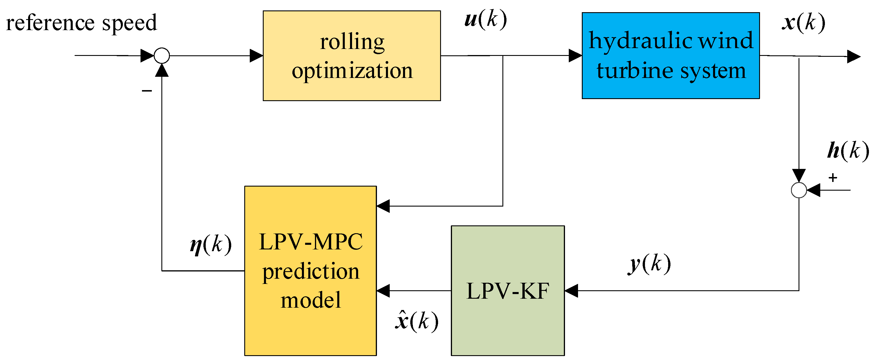
Considering the measurement noise and wind speed uncertainty, the KF was embedded in MPC based on the LPV model. The structure of the LPV-MPC with the KF method for the hydraulic wind turbine is shown in Figure 2. The state variables were estimated with a dynamic KF based on the LPV model to obtain the estimated value x ^ ( k ) . MPC calculated the optimal control input by solving the optimal problem according to the state estimate x ^ ( k ) and the reference speed.
Equation (27) was discretized using the forward Euler method with a sampling time of T s as follows:
x ( k + 1 ) = A d ( z ( k ) ) x ( k ) + B d u ( k ) y ( k ) = C d ( z ( k ) ) x ( k )
where k is the sampling instant, A d ( z ( k ) ) = I + A f ( z ( k ) ) T s , B d = B T s , C d = 0 0 1 0 0 0 0 0 0 1 0 0 .
Considering the noise produced in the hydraulic wind turbine system, the state space equation could be rewritten as:
x ( k + 1 ) = A d ( z ( k ) ) x ( k ) + B d u ( k ) + d ( k ) y ( k ) = C d x ( k ) + h ( k )
where d ( k ) is the system noise and h ( k ) is the measurement noise.
In order to provide more accurate state information to MPC and improve the control accuracy of the controller, the KF was designed to reduce the influence of external disturbances on the system. The KF was based on the LPV model as follows [29]:
x ^ e ( k | k 1 ) = A d ( z ( k 1 ) ) x ^ ( k 1 | k 1 ) + B d u ( k 1 ) P e ( k | k 1 ) = A d ( z ( k 1 ) ) P ( k 1 | k 1 ) A d T ( z ( k 1 ) ) + Q K F K K F ( k ) = P e ( k | k 1 ) C d T ( C d P e ( k | k 1 ) C d T + R K F ) 1 e ( k ) = y ( k ) ( C d x ^ e ( k | k 1 ) ) x ^ ( k | k ) = x ^ e ( k | k 1 ) + K K F ( k ) e ( k ) P ( k | k ) = ( I K K F ( k ) C d ) P ( k | k 1 )
in which the subscript “e” indicates the a priori estimate obtained before the measurement was updated. Q K F is the system noise covariance matrix and R K F is the measurement noise covariance matrix in the MPC state estimator.
In practical applications, the control inputs often adopt the incremental form:
Δ u ( k ) = u ( k ) u ( k 1 )
Therefore, Equations (27) and (30) were combined to construct the new state space expressions [30]:
ξ ( k + 1 ) = A ˜ d ( z ( k ) ) ξ ( k ) + B ˜ d Δ u ( k ) η ( k ) = C ˜ d ξ ( k )
where ξ ( k ) = x ^ ( k ) u ( k 1 ) , A ˜ d ( z ( k ) ) = A d ( z ( k ) ) B d 0 m × n I m , B ˜ d = B d I m , C ˜ d = C d 0 , n is the dimension of the state vector and m is the dimension of the control vector.
Suppose the control horizon was N C , the prediction horizon was N P and N C N P . The system output expression in the prediction horizon would be as follows:
Y ( k ) = Ψ ξ ( k ) + Θ Δ U ( k )
where
Y ( k ) = η ( k + 1 ) η ( k + N C ) η ( k + N P ) , Δ U ( k ) = Δ u ( k ) Δ u ( k + 1 ) Δ u ( k + N C 1 ) Δ u ( k + N C ) , Ψ = C ˜ d A ˜ d ( z ( k ) ) C ˜ d A ˜ d ( z ( k + 1 ) ) A ˜ d ( z ( k ) ) C ˜ d i = 0 N p 1 A ˜ d ( z ( k + i ) )
Θ = C ˜ d B ˜ d 0 0 0 C ˜ d A ˜ d ( z ( k ) ) B ˜ d C ˜ d B ˜ d 0 0 0 C ˜ d i = 1 N p 1 A ˜ d ( z ( k + i ) ) B ˜ d C ˜ d i = 2 N p 1 A ˜ d ( z ( k + i ) ) B ˜ d C ˜ d i = N C N p 1 A ˜ d ( z ( k + i ) ) B ˜ d
The control objective function of MPC was as follows:
J ( k ) = i = 1 N P Δ η ( k + i ) Q 2 + i = 1 N C 1 Δ u ( k + i ) R 2 + γ ε 2
where Q and R are positive definite weighting matrices, Δ η ( k + i ) = η ( k + i ) η r ( k + i ) , η r ( k + i ) is the target output sequence, γ is the weighting factor and ε is the relaxation factor. The last term was to ensure that the solver had a feasible solution for each control cycle.
The output deviation in the prediction horizon was:
E ( k ) = Y ( k ) Y r
where Y r = η r ( k + 1 ) η r ( k + 2 ) η r ( k + N P ) T .
In solving the quadratic programming optimization problem, the objective function needed to be transformed into the standard quadratic form and simplified as:
J ( k ) = 1 2 Δ U T ε T H Δ U T ε + G ( k + 1 | k ) Δ U T ε
where H = 2 Θ T Q Θ + 2 R 0 0 2 γ , G ( k + 1 | k ) = 2 E T Q Θ 0 .
The variable pump and variable motor speed was controlled within a reasonable range; thus, the normal operation of the hydraulic wind turbine could be guaranteed. Therefore, it was necessary to restrict control inputs in the following constraint form:
Δ U min Δ U ( k ) Δ U max U min U ( k ) + A I Δ U ( k ) U max
where U ( k ) = 1 N C u ( k 1 ) and is the Kronecker product.
After solving the quadratic programming in each calculation step, the sequence of incremental control inputs in the prediction horizon was obtained as:
Δ U ( k ) = Δ u * ( k )   Δ u * ( k + 1 )     Δ u * ( k + N C 1 ) T
Then, the control inputs were updated in the process of rolling optimization as follows:
u ( k ) = u ( k 1 ) + Δ u * ( k )
To prove the system stability at the equilibrium point, the Lyapunov function V * ( k ) , which corresponds to the optimal solution Δ u * ( k ) , was defined as [31]:
V * ( k ) = min Δ u i = 1 N P Δ η ( k + i ) Q 2 + i = 1 N C 1 Δ u ( k + i ) R 2
To facilitate analysis, it was assumed that N C = N P = N . Therefore, Equation (42) was simplified as follows:
V * ( k ) = min Δ u i = 1 N Δ η ( k + i ) Q 2 + Δ u ( k + i 1 ) R 2 s . t . Δ η ( k + i ) E Δ u ( k + i ) Δ U Δ η ( k + N ) = 0
where Δ U and E are nonempty sets. The function V * ( k ) was positive-definite.
With the above assumption, we had:
Δ V * ( k ) = V * ( k + 1 ) V * ( k ) = min Δ u Δ η ( k + 1 ) Q 2 Δ u ( k ) R 2 + Δ η ( k + 1 + N ) Q 2 + Δ u ( k + N ) R 2 Δ η ( k + 1 ) Q 2 Δ u * ( k ) R 2 + min Δ u Δ η ( k + 1 + N ) Q 2 + Δ u ( k + N ) R 2
According to the terminal constraint Δ η ( k + N ) = 0 , the following equation was concluded:
min Δ u Δ η ( k + 1 + N ) Q 2 + Δ u ( k + N ) R 2 = 0
Since Δ η ( k + 1 ) Q 2 + Δ u * ( k ) R 2 0 , we could conclude that Δ V * ( k ) 0 . According to Lyapunov’s stability theorem, the equilibrium point was stable.

4. Simulation Study and Results

In order to evaluate the performance of the proposed LPV model and controller, the system was simulated utilizing MATLAB/Simulink version R2018b software with an ode45 solver and quadratic program (QP) solver. The ode45 solver performed the integral solution of the differential equation and the QP solver was used to solve the MPC optimization problem.
The main parameters of the hydraulic wind turbine in the simulation are shown in Table 1. The parameters of the synchronous generator are listed in Table 2.
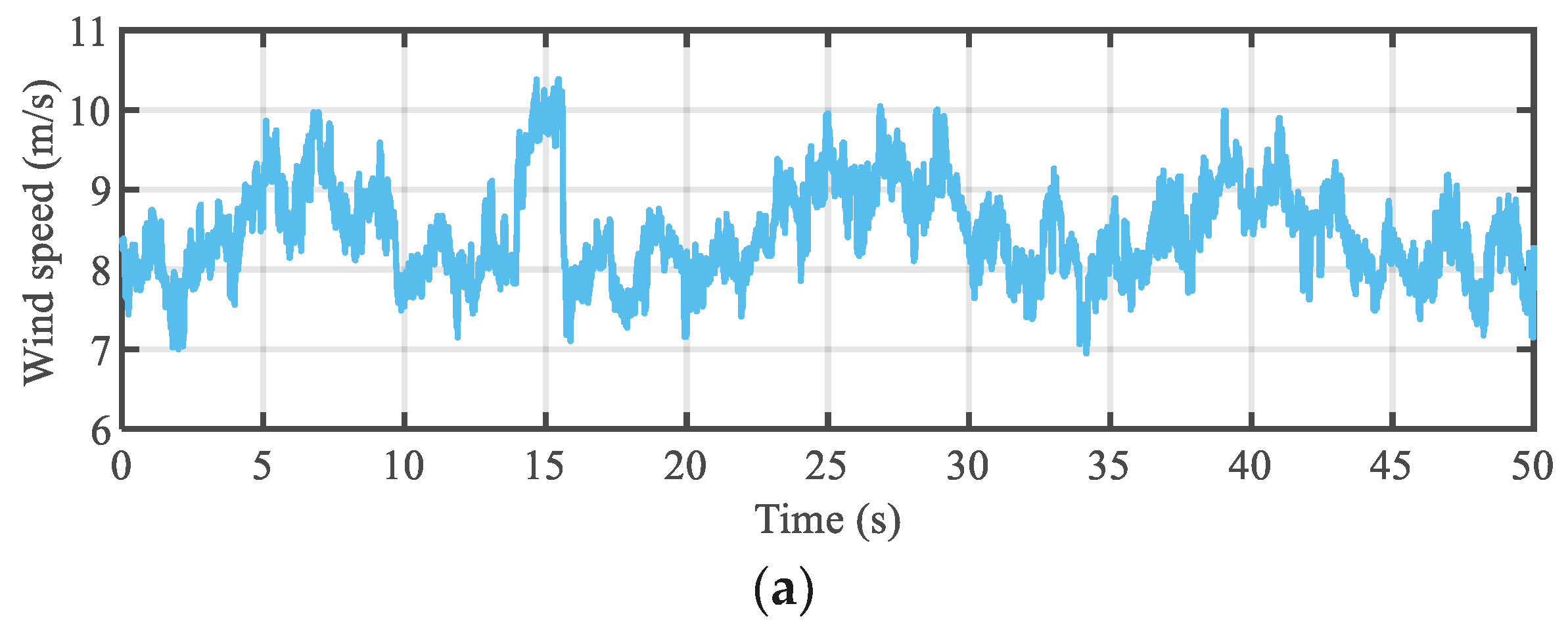
To detect the anti-interference ability of the whole control system when the wind speed changed, the simulations were conducted for 50 s in three simulation scenarios that covered different wind speeds and turbulence intensities.
Scenario 1: Mean wind speed of 8.3 m/s with an approximately 7.2% turbulence intensity.
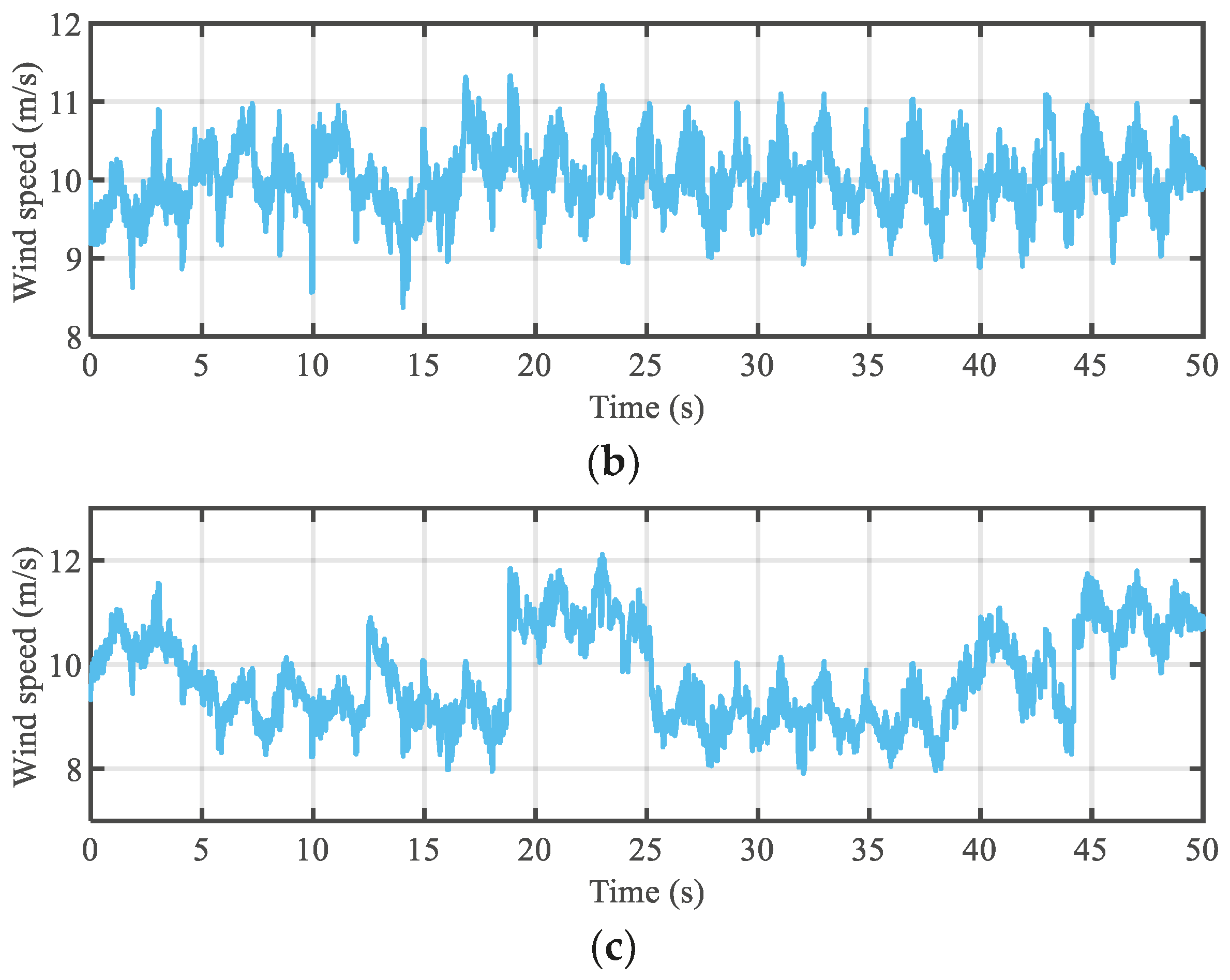
Scenario 2: Mean wind speed of 10 m/s (rated speed wind) with an approximately 5% turbulence intensity.
Scenario 3: Mean wind speed of 10 m/s (rated speed wind) with an approximately 10% turbulence intensity.
The turbulent wind speed curve with mean values 8.3 m/s and 10 m/s is shown in Figure 3. In addition, Gaussian white noise was introduced as the measurement noise in the simulation process.
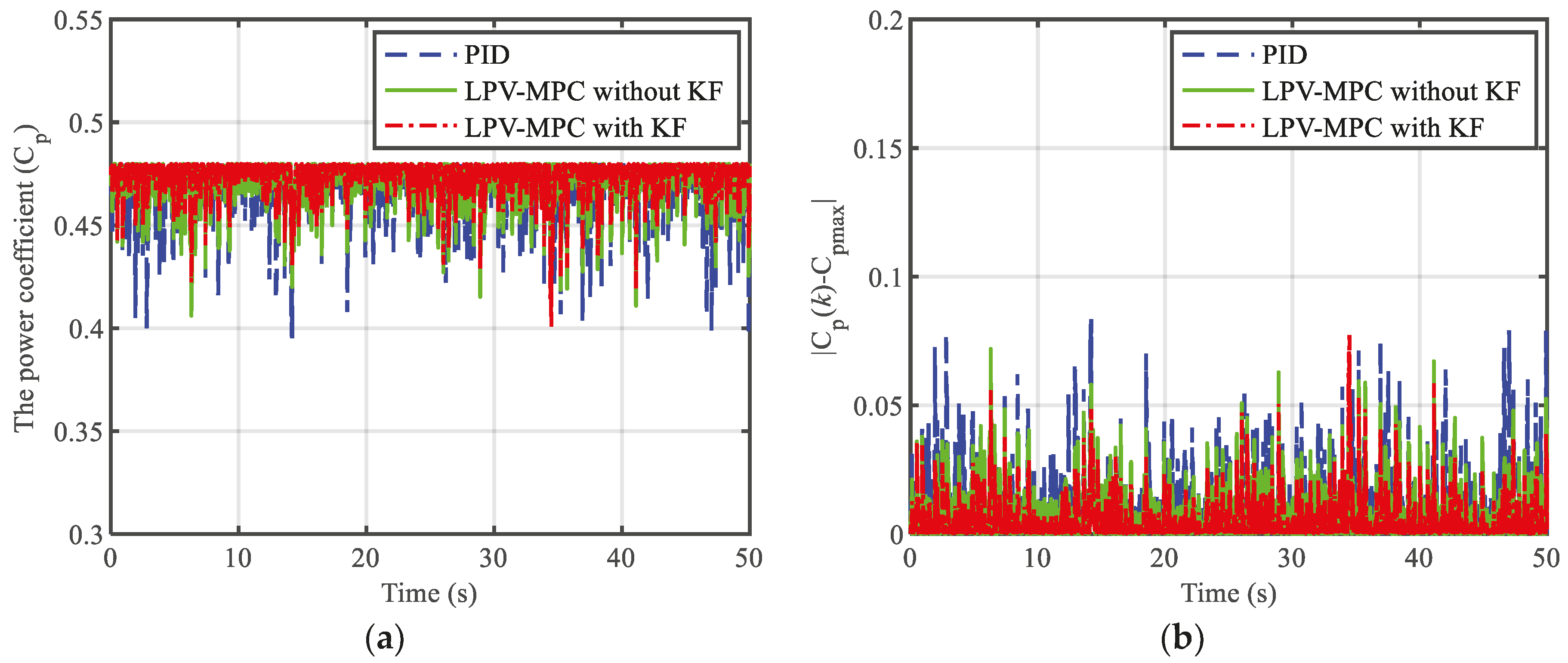
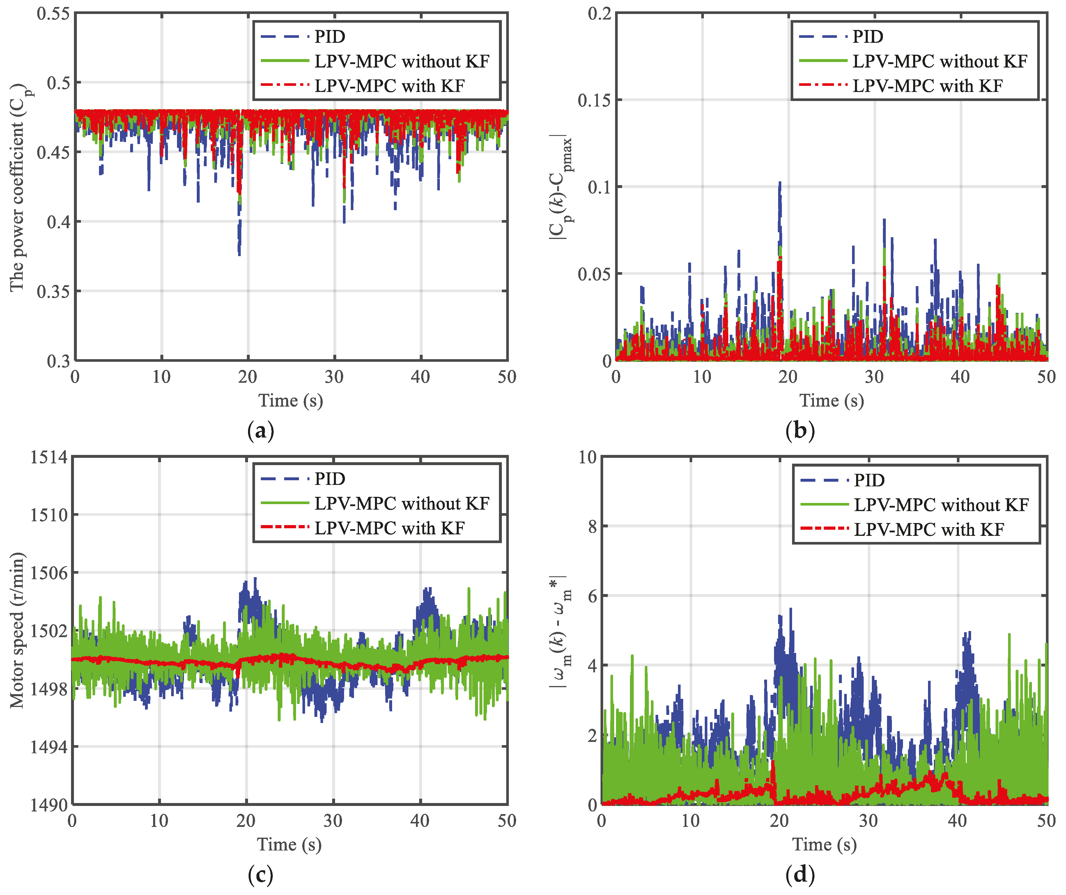
To examine the control performance of the LPV-MPC with the KF method, it was compared with the PID and the LPV-MPC without the KF method. The sampling time was set as T s = 0.01 s for both the LPV-MPC without the KF and the LPV-MPC with the KF in the following simulations. The controller parameters were N P = 6, N C = 3 and C p max = 0.478. The simulation results, including the power coefficients and the variable motor speed in each scenario, are shown in Figure 4, Figure 5 and Figure 6.
As shown in Figure 4, Figure 5 and Figure 6, compared with the PID and LPV-MPC without the KF method, the power coefficient was more stable around its maximum value under the LPV-MPC with the KF method. The variable motor speed was better maintained at the reference values when using the proposed method, whereas the motor speed fluctuated significantly when using the PID and LPV-MPC without the KF method in all scenarios. The results of Figure 5 and Figure 6 indicate that the absolute error of the variable motor speed under three control methods became larger with the increase in the turbulence intensity at the same wind speed. However, the LPV-MPC with the KF method could still keep the speed deviation within 1 r/min in scenario three, whereas the maximum speed deviation was approximately 4 r/min and 5.5 r/min, respectively, under the LPV-MPC without the KF method and PID method.
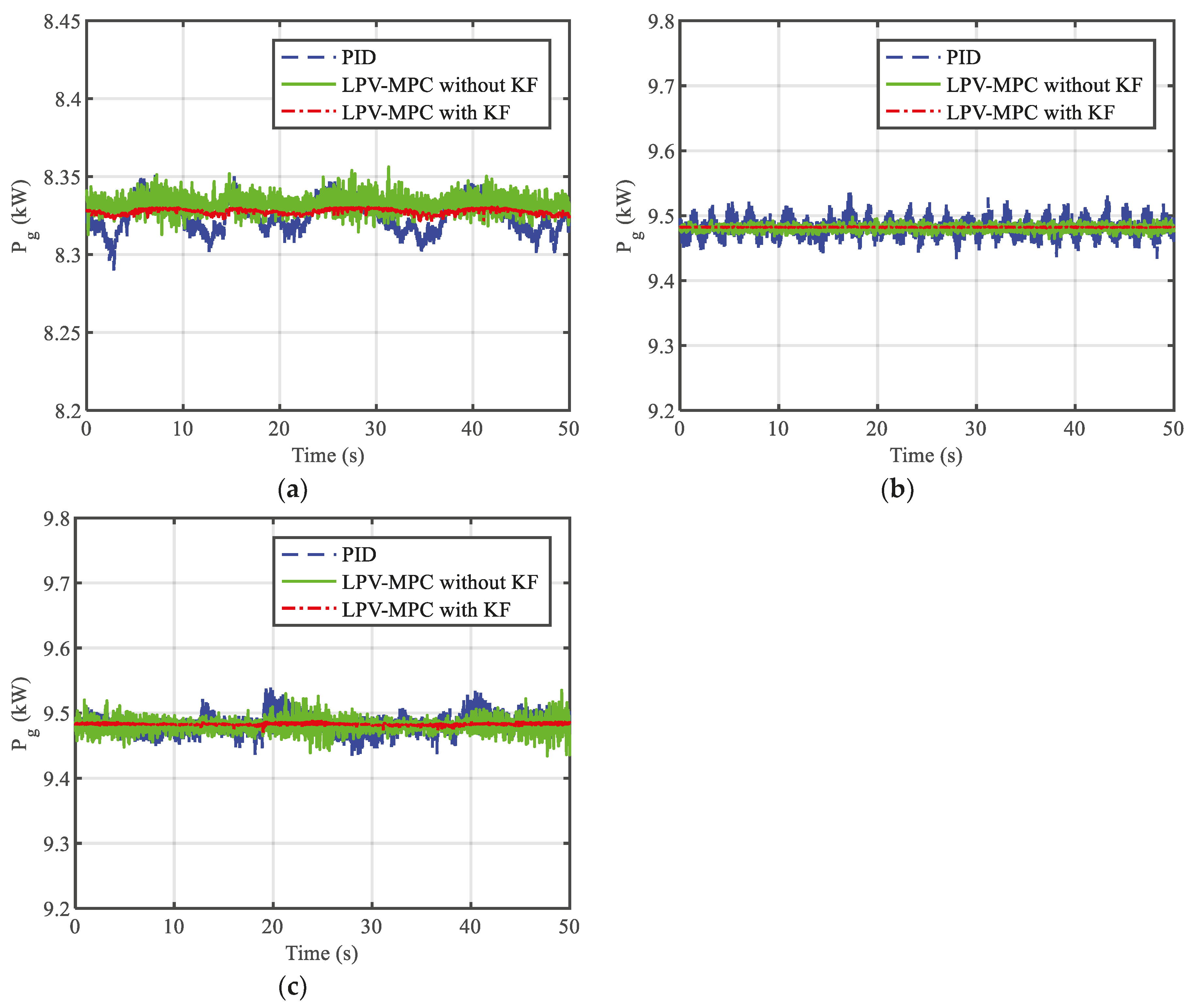
In order to explore the effect of the motor speed fluctuation on generator power, the generator power in all scenarios under the three control methods is shown in Figure 7. Figure 7 indicates that the variable motor speed and generator power had the similar fluctuation trend. The more stable the motor speed, the more stable the generator power. Through a comparison, it was found that the LPV-MPC with the KF method was better at keeping the generator power stable and ensuring the power quality more effectively.
In order to compare the performance of the methods of tracking the reference value in the case of the measurement noise and wind interference, the root mean square error (RMSE) was used to evaluate system control performance. The RMSE of the power coefficient, variable motor speed and generator power was defined as:
R M S E C p = 1 n k = 1 n C p ( k ) C p max 2
R M S E ω m = 1 n k = 1 n ω m ( k ) ω m * 2
R M S E P g = 1 n k = 1 n P g ( k ) P g * 2
where C p ( k ) , ω m ( k ) and P g ( k ) are the sampling values of the power coefficient, variable motor speed and generator power at the sample instant k, respectively. C p max is the maximal value of the power coefficient and ω m * and P g * are the reference values of variable motor speed and generator power at the sampling instant k, respectively. Table 3 summarizes the RMSE of the power coefficient, variable motor speed and generator power at different wind speeds with turbulence intensities.
Table 3 shows that the different turbulence intensity of the same wind speed had effects on the RMSE of the power coefficient, variable motor speed and generator power. The increase in the turbulence intensity of the same wind speed led to the increase in the power coefficient, variable motor speed and generator power fluctuation. Compared with the other two control methods, the hydraulic wind turbine system using the proposed method was more stable under turbulent wind. Take scenario three as an example: the LPV-MPC with the KF method decreased the RMSE of the power coefficient by 48.74% and 19.74%, the RMSE of the variable motor speed by 81.88% and 70.14%, and the RMSE of the generator power by 81.25% and 68.18%, respectively, in comparison with the PID and LPV-MPC without the KF methods. The simulation results indicated that the LPV-MPC with the KF had the best anti-interference performance among the three control methods.

5. Conclusions

In this paper, a LPV-MPC with the KF method was presented to establish a model and control for the hydraulic wind turbine. Firstly, the nonlinear model of the hydraulic wind turbine was transformed into the LPV model using function substitution. Secondly, a dynamic KF was designed to estimate the state variables and minimize model process mismatches based on the LPV model. Finally, the LPV model-based MPC with the KF was designed to control the variable pump speed and variable motor speed. The proposed method was compared with the PID and LPV-MPC without the KF method via a simulation under different wind speed disturbances and measurement noise conditions. The simulation results showed that both the LPV-MPC with the KF and the LPV-MPC without the KF methods outperformed the PID method under different wind speed disturbances. This indicated that the MPC method had the capability to react in advance and choose the optimal control input. The LPV-MPC with the KF used the Kalman filter to suppress measurement noise and wind disturbance, so that it obtained better anti-interference performance relative to the LPV-MPC without the KF method.
This paper studied the control of hydraulic wind turbines under fixed pitch angle conditions. Future research should focus on the combination of the proposed method in this paper and pitch control. Another future direction can be to study the fault-tolerant control method for hydraulic wind turbines based on the LPV in addressing the problem of sensor malfunctions.

Author Contributions

Conceptualization, B.H. and H.G.; methodology, B.H. and H.G.; software, B.H.; validation, B.H.; formal analysis, B.H.; investigation, B.H.; resources, B.H.; data curation, B.H.; writing—original draft preparation, B.H. and H.G.; writing—review and editing, H.G.; visualization, B.H.; supervision, H.G.; project administration, H.G.; funding acquisition, H.G. All authors have read and agreed to the published version of the manuscript.

Funding

This research received no external funding.

Data Availability Statement

Not applicable.

Conflicts of Interest

The authors declare no conflict of interest.

References

  1. Taherian-Fard, E.; Sahebi, R.; Niknam, T.; Izadian, A.; Shasadeghi, M. Wind Turbine Drivetrain Technologies. IEEE Trans. Ind. Appl. 2020, 56, 1729–1741. [Google Scholar] [CrossRef]
  2. Ribrant, J.; Bertling, L. Survey of Failures in Wind Power Systems with Focus on Swedish Wind Power Plants during 1997–2005. In Proceedings of the 2007 IEEE Power Engineering Society General Meeting, Tampa, FL, USA, 24–28 June 2007; pp. 1–8. [Google Scholar] [CrossRef]
  3. de Vries, E. Wind turbine drive systems: A commercial overview. Electr. Drives Direct Drive Renew. Energy Syst. 2013, 139–157. [Google Scholar] [CrossRef]
  4. Polinder, H.; van der Pijl, F.F.A.; de Vilder, G.J.; Tavner, P.J. Comparison of direct-drive and geared generator concepts for wind turbines. IEEE Trans. Energy Convers. 2006, 21, 725–733. [Google Scholar] [CrossRef] [Green Version]
  5. Yin, X.; Zhang, W.; Zhao, X. Current status and future prospects of continuously variable speed wind turbines: A systematic review. Mech. Syst. Signal Process. 2019, 120, 326–340. [Google Scholar] [CrossRef]
  6. Mohanty, B.; Stelson, K.A. Experimental validation of a hydrostatic transmission for community wind turbines. Energies 2022, 15, 376. [Google Scholar] [CrossRef]
  7. Laguna, A.J. Modeling and Analysis of an Offshore Wind Turbine With Fluid Power Transmission for Centralized Electricity Generation. J. Comput. Nonlinear Dyn. 2015, 10, 041002. [Google Scholar] [CrossRef]
  8. Lin, S.; Zhao, X.; Tong, X. Feasibility Studies of a Converter-Free Grid-Connected Offshore Hydrostatic Wind Turbine. IEEE Trans. Sustain. Energy 2020, 11, 2494–2503. [Google Scholar] [CrossRef] [Green Version]
  9. Farbood, M.; Taherian-Fard, E.; Shasadeghi, M.; Izadian, A.; Niknamet, T. Dynamics and Control of a Shared Wind Turbine Drivetrain. IEEE Trans. Ind. Appl. 2018, 54, 6394–6400. [Google Scholar] [CrossRef]
  10. Dolan, B.; Aschemann, H. Control of a wind turbine with a hydrostatic transmission—An extended linearisation approach. In Proceedings of the 2012 17th International Conference on Methods and Models in Automation and Robotics (MMAR), Miedzyzdrojie, Poland, 27–30 August 2012. [Google Scholar] [CrossRef]
  11. Ai, C.; Zhou, G.; Gao, W.; Guo, J.; Jie, G.; Han, Z.; Kong, X. Research on Quasi-Synchronous Grid-Connected Control of Hydraulic Wind Turbine. IEEE Access 2020, 8, 126092–126108. [Google Scholar] [CrossRef]
  12. Gao, W.; Lijuan, C.; Chao, A.; Pengfei, Z.; Xuan, W. Research on Active Power Online Optimal Control for Hydrostatic Transmission Wind Turbine. IEEE Access 2021, 10, 54263–54275. [Google Scholar] [CrossRef]
  13. Rugh, W.J.; Shamma, J.S. Research on gain scheduling. Automatica 2000, 36, 1401–1425. [Google Scholar] [CrossRef]
  14. Hu, Y.; Duan, G.; Tan, F. Finite-time control for LPV systems with parameter-varying time delays and exogenous disturbances. Int. J. Robust Nonlinear Control 2017, 27, 3841–3861. [Google Scholar] [CrossRef]
  15. Morato, M.M.; Normey-Rico, J.E.; Sename, O. Model predictive control design for linear parameter varying systems: A survey. Elsevier Annu. Rev. Control 2020, 49, 64–80. [Google Scholar] [CrossRef]
  16. Marcos, A.; Balas, G.J. Development of Linear-Parameter-Varying Models for Aircraft. J. Guid. Control Dyn. 2004, 27, 218–288. [Google Scholar] [CrossRef] [Green Version]
  17. Liu, Z.; Tao, Y.; Wei, L.; Zhan, P.; Yue, D. Analysis of Dynamic Characteristics of a 600 kW Storage Type Wind Turbine with Hybrid Hydraulic Transmission. Processes 2019, 7, 397. [Google Scholar] [CrossRef] [Green Version]
  18. Fan, Y.J.; Mu, A.L. Adaptive fuzzy Proportion Integration Differentiation control in hydraulic offshore wind turbine for optimal power extraction based on the estimated wind speed. Energy Sci. Eng. 2020, 8, 1604–1619. [Google Scholar] [CrossRef] [Green Version]
  19. Schulte, H.; Gauterin, E. Fault-tolerant control of wind turbines with hydrostatic transmission using Takagi–Sugeno and sliding mode techniques. Annu. Rev. Contr. 2015, 40, 82–92. [Google Scholar] [CrossRef]
  20. Yu-Geng, X.; De-Wei, L.; Shu, L. Model predictive control—status and challenges. Acta Autom. Sin. 2013, 39, 222–236. [Google Scholar] [CrossRef]
  21. Sariyildiz, E.; Oboe, R.; Ohnishi, K. Disturbance Observer-Based Robust Control and Its Applications: 35th Anniversary Overview. IEEE Trans. Ind. Electron. 2020, 67, 2042–2053. [Google Scholar] [CrossRef] [Green Version]
  22. Yang, G.; Yao, J.; Ullah, N. Neuroadaptive control of saturated nonlinear systems with disturbance compensation. ISA Trans. 2022, 122, 49–62. [Google Scholar] [CrossRef]
  23. Yang, G.; Yao, J.; Dong, Z. Neuroadaptive learning algorithm for constrained nonlinear systems with disturbance rejection. Int. J. Robust Nonlinear Control 2022, 32, 6127–6147. [Google Scholar] [CrossRef]
  24. Koch, S.; Reichhartinger, M. Observer-based sliding mode control of hydraulic cylinders in the presence of unknown load forces. e i Elektrotechnik Inf. 2016, 133, 253–260. [Google Scholar] [CrossRef] [Green Version]
  25. Heier, S. Grid Integration of Wind Energy: Onshore and Offshore Conversion Systems, 3rd ed.; John Wiley & Sons: Chichester, UK, 2014; pp. 43–44. ISBN 978-1-119-96294-6. [Google Scholar]
  26. Wei, L.; Liu, Z.; Zhao, Y.; Wang, G.; Tao, Y. Modeling and Control of a 600 kW Closed Hydraulic Wind Turbine with an Energy Storage System. Appl. Sci. 2018, 8, 1314. [Google Scholar] [CrossRef] [Green Version]
  27. Ai, C.; Gao, W.; Chen, L.; Guo, J.; Kong, X.; Plummer, A. Bivariate grid-connection speed control of hydraulic wind turbines. J. Franklin Inst. 2021, 358, 296–320. [Google Scholar] [CrossRef]
  28. Bottiglione, F.; Mantriota, G.; Valle, M. Power-Split Hydrostatic Transmissions for Wind Energy Systems. Energies 2018, 11, 3369. [Google Scholar] [CrossRef] [Green Version]
  29. Uchihori, H.; Cavanini, L.; Tasaki, M. Linear Parameter-Varying Model Predictive Control of AUV for Docking Scenarios. Appl. Sci. 2021, 11, 4368. [Google Scholar] [CrossRef]
  30. Gong, J.W.; Xu, W.; Jiang, Y.; Liu, K.; Guo, H.F.; Sun, Y.J. Multi-constrained model predictive control for autonomous ground vehicle trajectory tracking. J. Beijing Inst. Technol. 2015, 24, 441–443. [Google Scholar]
  31. Maciejowski, J.M. Predictive Control: With Constraints; Prentice-Hall: Harlow, UK, 2002. [Google Scholar]
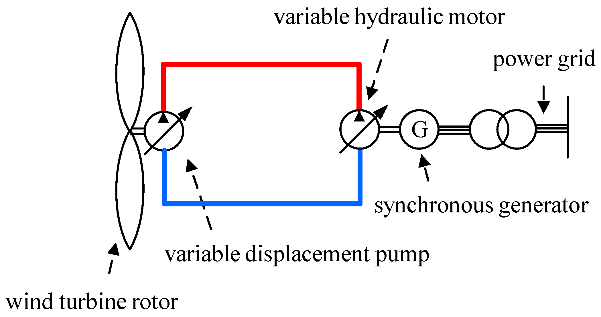
Figure 1. A schematic diagram of the hydraulic wind turbine.
Actuators 11 00292 g001
Figure 2. Structure of the LPV-MPC with the KF method for the hydraulic wind turbine.
Actuators 11 00292 g002
Figure 3. Turbulent wind speed curve: (a) mean wind speed of 8.3 m/s with approximately 7.2% turbulence intensity; (b) mean wind speed of 10 m/s with approximately 5% turbulence intensity; (c) mean wind speed of 10 m/s with approximately 10% turbulence intensity.
Actuators 11 00292 g003aActuators 11 00292 g003b
Figure 4. Comparison of power coefficients and variable motor speeds under different control methods in scenario 1: (a) power coefficient; (b) absolute error of power coefficient; (c) variable motor speeds; (d) absolute error of variable motor speeds.
Actuators 11 00292 g004aActuators 11 00292 g004b
Figure 5. Comparison of power coefficients and variable motor speeds under different control methods in scenario 2: (a) power coefficient; (b) absolute error of power coefficient; (c) variable motor speeds; (d) absolute error of variable motor speeds.
Actuators 11 00292 g005
Figure 6. Comparison of power coefficients and variable motor speeds under different control methods in scenario 3: (a) power coefficient; (b) absolute error of power coefficient; (c) variable motor speeds; (d) absolute error of variable motor speeds.
Actuators 11 00292 g006
Figure 7. Comparison of generator power under different control methods: (a) scenario 1; (b) scenario 2; (c) scenario 3.
Actuators 11 00292 g007
Table 1. Main parameters of the hydraulic wind turbine.
SymbolParameterValueUnit
RRotor radius4m
ρ Air density1.225kg/m3
JpThe total inertia of the rotor in the wind turbine and pump8kg·m2
BpDamping coefficient of the pump0.02N·m/(rad·s−1)
DPPump displacement300ml
DmMotor displacement35ml
BmDamping coefficient of the motor0.009N·m/(rad·s−1)
JmThe total inertia of the rotor in the variable motor and generator0.1278kg·m2
β e The effective bulk modulus of hydraulic oil1.43 × 103MPa
CvTotal system leakage coefficient8 × 10−12m3/(s·Pa)
VThe total compression volume0.05m3
τ g The time constant of the generator0.02s
τ p The time constant of the pump0.1s
τ m The time constant of the motor0.1s
Table 2. Synchronous generator parameters.
ParameterValueUnit
Stator resistance0.645Ω
Inductance3.371mH
Pole pairs2-
Synchronous speed1500r/min
Rated line voltage380V
Rated power10kW
ηg95%-
Table 3. RMSE at different wind speeds with turbulence intensities.
ScenarioWind
Speed
Turbulence
Intensity
RMSEPIDLPV-MPCLPV-MPC with KF
18.3 m/s7.2% R M S E C p 0.01330.01150.0086
R M S E ω m 1.55560.96940.2653
R M S E P g 0.01070.00690.0017
210 m/s5% R M S E C p 0.00780.00670.0049
R M S E ω m 1.22530.68670.0558
R M S E P g 0.01060.00450.0005
310 m/s10% R M S E C p 0.01190.00760.0061
R M S E ω m 1.67851.01880.3042
R M S E P g 0.01120.00660.0021
Publisher’s Note: MDPI stays neutral with regard to jurisdictional claims in published maps and institutional affiliations.