Reliability Analysis of Reinforced Concrete Frame by Finite Element Method with Implicit Limit State Functions


Abstract
1. Introduction
Reliability Analysis Methods
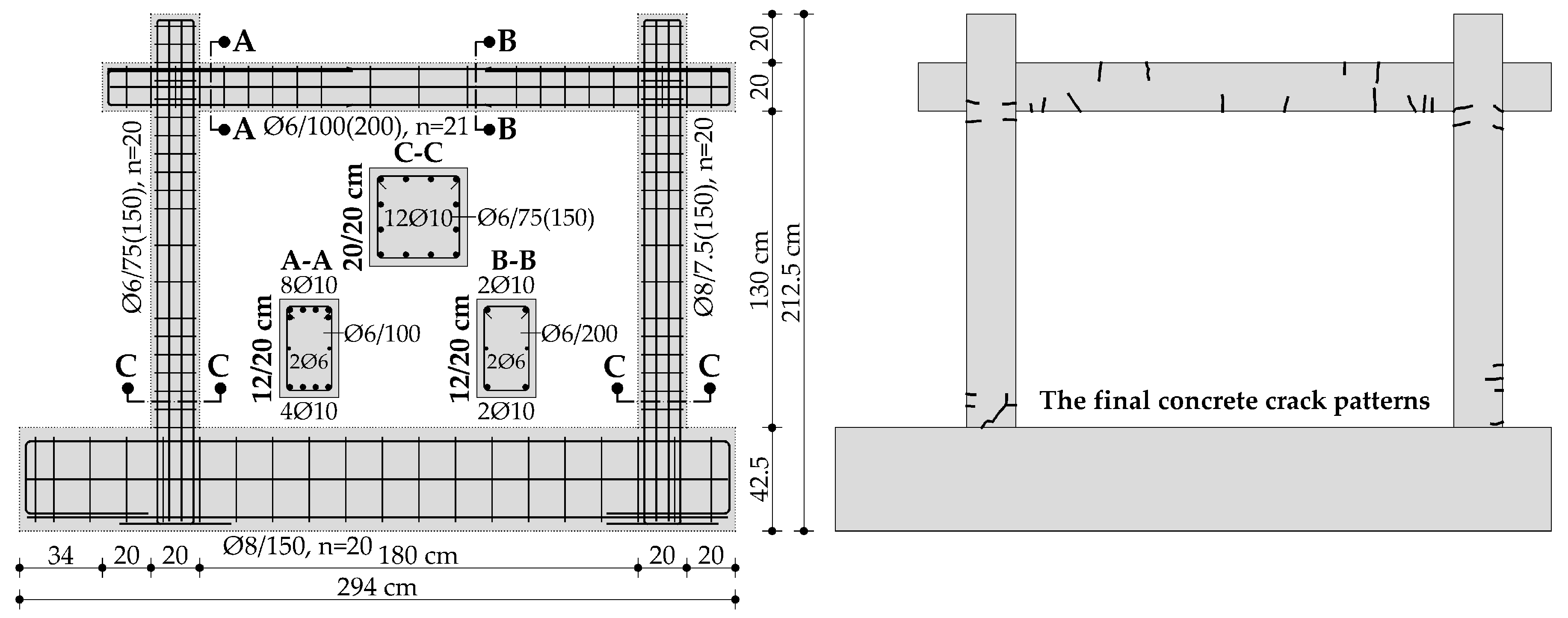
2. Experimental Model
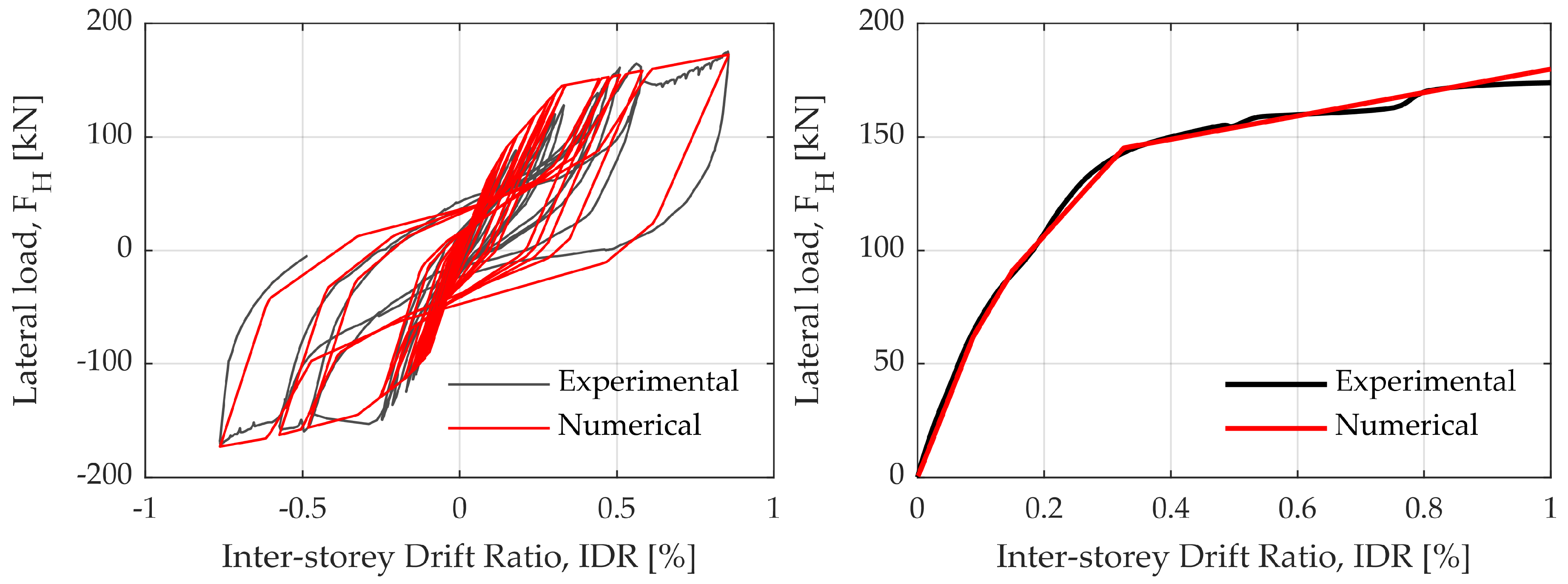
3. Numerical Model
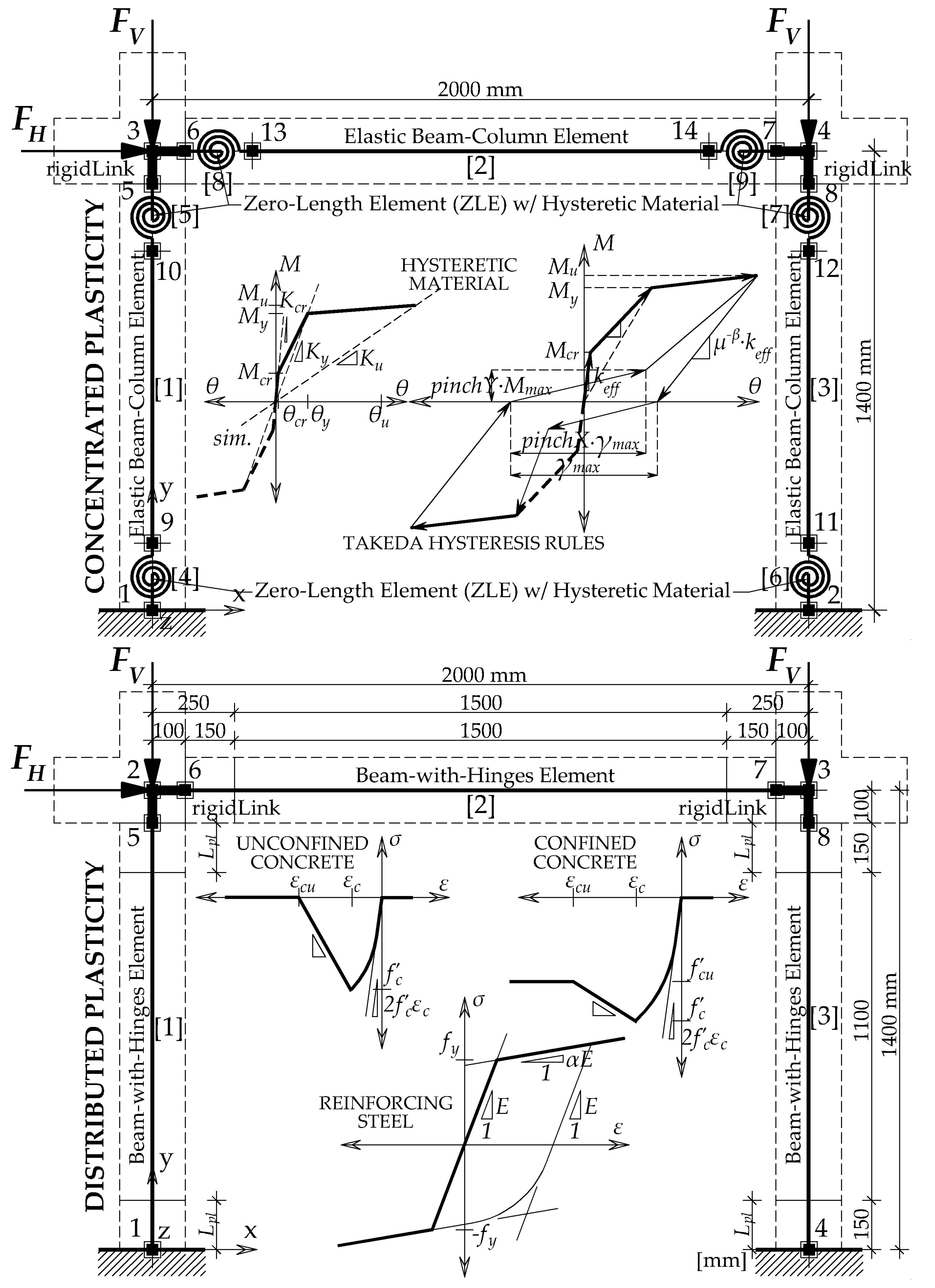
3.1. Concentrated (Lumped) Plasticity Model (CP)
3.2. Distributed Plasticity Model (DP)
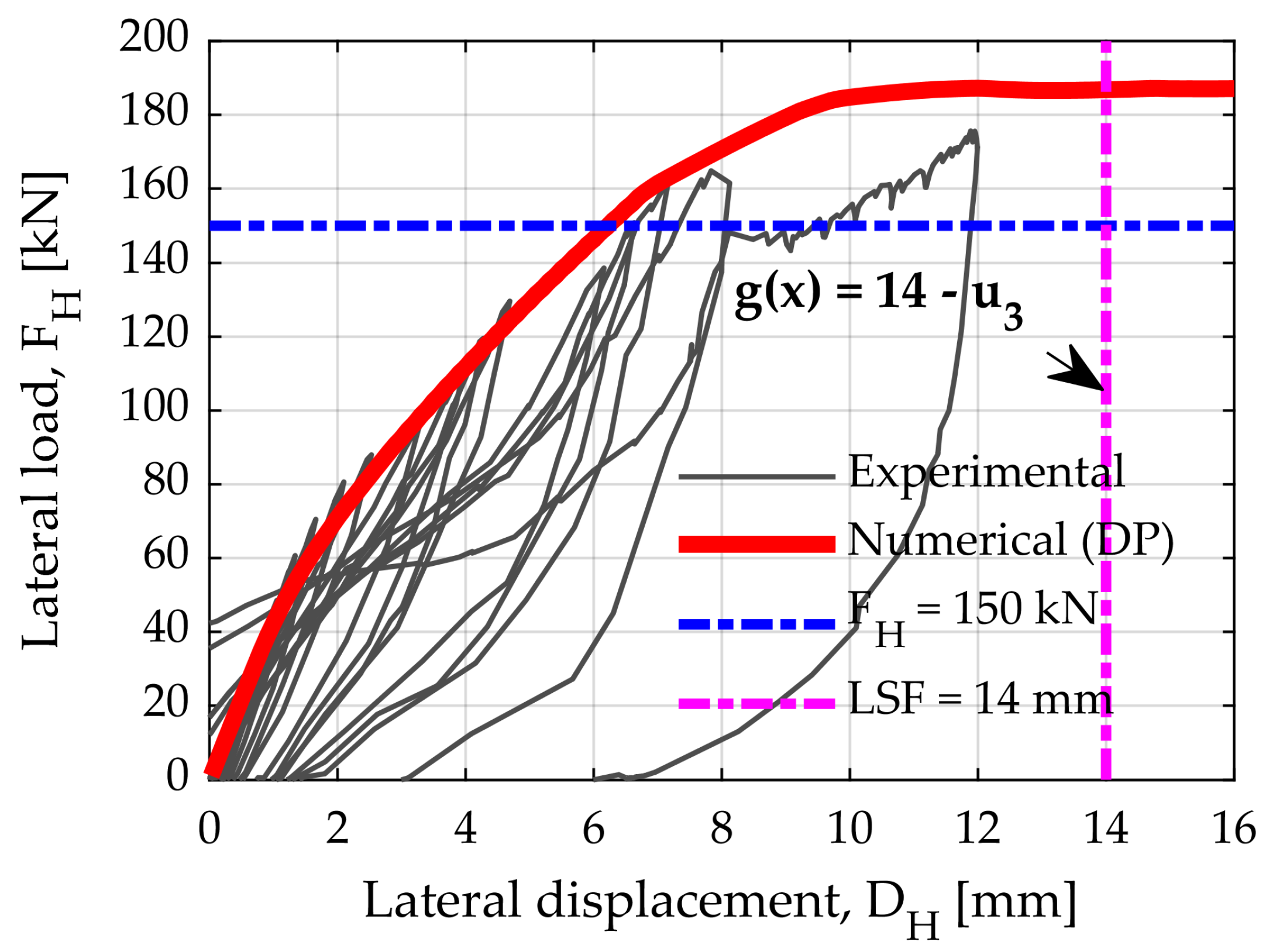
4. Reliability Analysis
5. Reliability Analyses Results
5.1. MVFOSM, FORM, and SORM Analyses
5.2. Monte Carlo Simulations
6. Conclusions
Author Contributions
Funding
Acknowledgments
Conflicts of Interest
Abbreviations
| COV | Coefficients Of Variation |
| CP | Concentrated Plasticity |
| DC | Displacement control |
| DCM | Ductility Class Medium |
| DOF | Degree-Of-Freedom |
| DP | Distributed Plasticity |
| E | Effect (Load) |
| EDP | Engineering Demand Parameter |
| FEM | Finite Element Method |
| FORM | First-Order Reliability Method |
| HLRF | Hasofer–Lind–Rackwitz–Fiessler |
| IDR | Inter-storey Drift Ratio |
| IM | Intensity Measure |
| LC | Load Control |
| LHS | Latin Hypercube Sampling |
| LN | Log-normal distribution |
| LSF | Limit State Function |
| MCS | Monte Carlo Simulation |
| MCS-DC | Monte Carlo Simulation, Displacement control |
| MCS-LC | Monte Carlo Simulation, Load control |
| MPP | Most Probable Point |
| MVFOSM | Mean-Value First-Order Second-Moment |
| N | Normal distribution |
| PACT | Performance Assessment Calculation Tool |
| PBEE | Performance-Based Earthquake Engineering |
| Probability Density Function | |
| PEER | Pacific Earthquake Engineering Research |
| PGA | Peak Ground Acceleration |
| R | Resistance (Bearing Capacity) |
| RC | Reinforced Concrete |
| RSM | Response Surface Method |
| RV | Random Variables |
| SDOF | Single Degree-Of-Freedom |
| SORM | Second Order Reliability Method |
| SORM-CF | Second-Order Reliability Method, Curvature Fitting |
| SORM-FP | Second-Order Reliability Method, First Principal Curvature |
| TDA | Tornado Diagram Analysis |
References
- Huang, C.; El Hami, A.; Radi, B. Overview of Structural Reliability Analysis Methods—Part I: Local Reliability Methods. Incert. Fiabil. Syst. Multiphys. 2017, 17, 1–10. [Google Scholar] [CrossRef]
- Hami, A.E.; Radi, B. Uncertainty and Optimization in Structural Mechanics; John Wiley & Sons, Inc.: Hoboken, NJ, USA, 2013; p. 138. [Google Scholar]
- Lemaire, M.; Chateauneuf, A.; Mitteau, J. Structural Reliability; ISTE Ltd., Wiley: Hoboken, NJ, USA, 2009; p. 485. [Google Scholar] [CrossRef]
- Grubišić, M. Models for Strengthening Assessment of Reinforced Concrete Frames by Adding the Infills for Earthquake Action. Ph.D. Thesis, University of Osijek, Faculty of Civil Engineering Osijek, Osijek, Croatia, 2016. [Google Scholar]
- McKenna, F.; Fenves, G.L.; Scott, M.H.; Mazzoni, S.; Jeremić, B. OpenSees—Open System for Earthquake Engineering Simulation; Technical report; Pacific Earthquake Engineering Research Centre, PEER, University of California: Berkeley, CA, USA, 2000. [Google Scholar]
- Datta, T.K. Seismic Analysis of Structures; John Wiley & Sons (Asia) Pte Ltd.: Singapore, 2010; p. 451. [Google Scholar] [CrossRef]
- Miranda, J. Structural Reliability Analysis with Implicit Limit State Functions; Technical Report; Instituto Superior Técnico, University of Lisbon: Lisbon, Portugal, 2013. [Google Scholar]
- Bozorgnia, Y.; Bertero, V. Earthquake Engineering: From Engineering Seismology to Performance—Based Engineering; CRC Press, ICC (International Code Council): Boca Raton, FL, USA, 2004. [Google Scholar]
- Deierlein, G.G.; Krawinkler, H.; Cornell, C.A. A Framework for Performance-Based Earthquake Engineering. Pac. Conf. Earthq. Eng. 2003, 273, 1–8. [Google Scholar] [CrossRef]
- Günay, S.; Mosalam, K.M. PEER Performance-Based Earthquake Engineering Methodology, Revisited. J. Earthq. Eng. 2013, 17, 829–858. [Google Scholar] [CrossRef]
- FEMA-P58/1. Seismic Performance Assessment of Buildings—Volume 1—Methodology; Technical Report; Applied Technology Council, Ed.; Federal Emergency Management Agency, FEMA & NEHRP: Washington, DC, USA, 2012.
- Sigmund, V.; Penava, D. Influence of Openings, with and Without Confinement, on Cyclic Response of Infilled R-C Frames—An Experimental Study. J. Earthq. Eng. 2014, 18, 113–146. [Google Scholar] [CrossRef]
- Kalman Šipoš, T.; Sigmund, V.; Hadzima-Nyarko, M. Earthquake performance of infilled frames using neural networks and experimental database. Eng. Struct. 2013, 51, 113–127. [Google Scholar] [CrossRef]
- Kabeyasawa, T.; Shiohara, H.; Otani, S.; Aoyama, H. Analysis of The Full–Scale Seven–Story Reinforced Concrete Test Structure. J. Fac. Eng. Univ. Tokyo Japan 1983, 37, 431–478. [Google Scholar]
- EN1992-1:2004. Eurocode 2—Design of Concrete Structures: General Rules and Rules for Buildings; European Committee for Standardization, CEN: Brussels, Belgium, 2004. [Google Scholar]
- EN1998-1:2004. Eurocode 8—Design of Structures for Earthquake Resistance—Part 1: General Rules, Seismic Actions and Rules for Buildings; European Committee for Standardization, CEN: Brussels, Belgium, 2004. [Google Scholar]
- Takeda, T.; Sozen, M.A.; Nielsen, N.N. Reinforced Concrete Response to Simulated Earthquakes. J. Struct. Div. 1970, 96, 2557–2573. [Google Scholar]
- Paulay, T.; Priestley, M.J.N. Seismic Design of Reinforced Concrete and Masonry Buildings, 1st ed.; Wiley, John Wiley & Sons, Inc.: Hoboken, NJ, USA, 1992; p. 735. [Google Scholar] [CrossRef]
- Scott, M.H.; Fenves, G.L.; McKenna, F.; Filippou, F.C. Software Patterns for Nonlinear Beam-Column Models. J. Struct. Eng. 2008, 134, 562–571. [Google Scholar] [CrossRef]
- Yaw, L.L. Co-Rotational Meshfree Formulation for Large Deformation Inelastic Analysis of Two-Dimensional Structural Systems. Ph.D. Thesis, University of California Davis, Davis, CA, USA, 2008. [Google Scholar]
- Denavit, M.D.; Hajjar, J.F. Description of Geometric Nonlinearity for Beam-Column Analysis in OpenSees; Technical report; Northeastern University: Boston, MA, USA, 2013. [Google Scholar]
- Rinchen; Hancock, G.J.; Rasmussen, K.J. Formulation and Implementation of General Thin-Walled Open-Section Beam-Column Elements in OpenSees; Technical Report 961; School of Civil Engineering, The University of Sydney: Sydney, Australia, 2016. [Google Scholar]
- Scott, M.H.; Fenves, G.L. Plastic Hinge Integration Methods for Force-Based Beam-Column Elements. J. Struct. Eng. 2006, 132, 244–252. [Google Scholar] [CrossRef]
- Scott, M.H.; Ryan, K.L. Moment-Rotation Behavior of Force-Based Plastic Hinge Elements. Earthq. Spectra 2013, 29, 597–607. [Google Scholar] [CrossRef]
- Haukaas, T.; Scott, M.H. Shape sensitivities in the reliability analysis of nonlinear frame structures. Comput. Struct. 2006, 84, 964–977. [Google Scholar] [CrossRef]
- Scott, M.H.; Haukaas, T. Software Framework for Parameter Updating and Finite-Element Response Sensitivity Analysis. J. Comput. Civ. Eng. 2008, 22, 281–291. [Google Scholar] [CrossRef]
- Scott, M.H. Evaluation of Force-Based Frame Element Response Sensitivity Formulations. J. Struct. Eng. 2011, 138, 72–80. [Google Scholar] [CrossRef]
- Deng, J.; Gu, D.; Li, X.; Yue, Z.Q. Structural reliability analysis for implicit performance functions using artificial neural network. Struct. Saf. 2005, 27, 25–48. [Google Scholar] [CrossRef]
- Hess, P.E.; Bruchman, D.; Assakkaf, I.A.; Ayyub, B.M. Uncertainties in Material and Geometric Strength and Load Variables. Nav. Eng. J. 2002, 114, 139–166. [Google Scholar] [CrossRef]
- Buonopane, S.G. Strength and Reliability of Steel Frames with Random Properties. J. Struct. Eng. 2008, 134, 337–344. [Google Scholar] [CrossRef]
- JCSS. Probabilistic Model Code Part III; Technical report; Technical University of Denmark, Joint Committee on Structural Safety (JCSS): Kongens Lyngby, Denmark, 2000. [Google Scholar]
- Celarec, D.; Ricci, P.; Dolšek, M. The sensitivity of seismic response parameters to the uncertain modelling variables of masonry-infilled reinforced concrete frames. Eng. Struct. 2012, 35, 165–177. [Google Scholar] [CrossRef]
- Ellingwood, B.; Galambos, T.; MacGregor, J.; Cornell, C.A. Development of a Probability—Based Load Criterion for American National Standard A58; Technical Report; National Bureau of Standards: Washington, DC, USA, 1980.
- El-Reedy, M.A. Reinforced Concrete Structural Reliability; CRC Press, Taylor & Francis Group: Boca Raston, FL, USA, 2013; p. 369. [Google Scholar]
- Robertson, L.E.; Naka, T. Tall Building Criteria and Loading; American Society of Civil Engineers: New York, NY, USA, 1980; p. 900. [Google Scholar]
- Mishra, D.K. Compressive Strength Variation of Concrete in a Large Inclined RC Beam by Non-Destructive Testing; Technical report; Associated Cement Companies Ltd.: Mumbai, India, 1990. [Google Scholar]
- Obla, K. Variation in Concrete Strength Due to Cement—Part III of Concrete Quality Series. Improv. Concr. Qual. 2014, 9, 7–16. [Google Scholar] [CrossRef]
- Sundararajan, C. Probabilistic Structural Mechanics Handbook: Theory and Industrial Applications; Springer: New York, NY, USA, 1995; p. 745. [Google Scholar] [CrossRef]
- Bartlett, F.M.; MacGregor, J.G. Assessment of Concrete Strength in Existing Structures; Technical Report; Department of Civil Engineering, University of Alberta: Edmonton, AB, Canada, 1994. [Google Scholar]
- Haukaas, T.; Kiureghian, A.D. Finite Element Reliability and Sensitivity Methods for Performance—Based Earthquake Engineering; Technical report, Pacific Earthquake PEER Report 2003/14; Engineering Research Centre, PEER, University of California: Berkeley, CA, USA, 2004. [Google Scholar]
- Porter, K.A.; Beck, J.L.; Shaikhutdinov, R.V. Sensitivity of Building Loss Estimates to Major Uncertain Variables. Earthq. Spectra 2002, 18, 719–743. [Google Scholar] [CrossRef]
- Celarec, D.; Dolšek, M. The impact of modelling uncertainties on the seismic performance assessment of reinforced concrete frame buildings. Eng. Struct. 2013, 52, 340–354. [Google Scholar] [CrossRef]
- Porter, K. A Beginner’s Guide to Fragility, Vulnerability, and Risk; Technical report; University of Colorado Boulder: Boulder, CO, USA; SPA Risk LLC: Denver, CO, USA, 2019. [Google Scholar]
- EN1990-1:2002. Eurocode 0—Basis of Structural Design; European Committee for Standardization, CEN: Brussels, Belgium, 2002. [Google Scholar]
- Python. Python Language Reference; Version 3.6.8, [MSC v.1916 64 bit (AMD64)]; Python Software Foundation: Wilmington, DE, USA, 2018. [Google Scholar]
- MATLAB. The MathWorks, Inc.; Version 9.4 (R2018a); The MathWorks, Inc.: Natick, MA, USA, 2018. [Google Scholar]
- Lee, T.H.; Mosalam, K.M. Probabilistic Seismic Evaluation of Reinforced Concrete Structural Components and Systems; Technical report, PEER Report 2006/04; Pacific Earthquake Engineering Research Centre, College of Engineering, PEER, University of California: Berkeley, CA, USA, 2006. [Google Scholar]
- Huang, Y.; Whittaker, A.S.; Luco, N. Performance Assessment of Conventional and Base-Isolated Nuclear Power Plants for Earthquake and Blast Loadings; Technical Report MCEER-08-0019; University of Buffalo: Buffalo, NY, USA, 2008. [Google Scholar]


| RV | Param. | Mean, | St. Dev., | COV | Units | Distr. | References for COV |
|---|---|---|---|---|---|---|---|
| 101 | 550 | 44 | 0.08 | (MPa) | LN | Experiment + [30,31,32] | |
| 102 | 210,000 | 12,600 | 0.06 | (MPa) | LN | Experiment + [26,29,30] | |
| 103 | −65 | −9.75 | 0.15 | (MPa) | N | Experiment + [30,33,34,35,36] | |
| 104 | −0.005 | −0.0008 | 0.15 | (−) | N | Experiment + [30,33,34,35,36,37] | |
| 105 | −50 | −7.5 | 0.15 | (MPa) | N | Experiment + [30,33,35,36] | |
| 106 | −0.002 | −0.0003 | 0.15 | (−) | N | Experiment + [30,33,37] | |
| 107 | −11.5 | −2.3 | 0.20 | (MPa) | N | Experiment + [30,33,34,35,36] | |
| 108 | −0.0085 | −0.0017 | 0.20 | (−) | N | Experiment + [30,33,34,35,36,37] | |
| 109 | −10 | −2 | 0.20 | (MPa) | N | Experiment + [30,33,35,36] | |
| 110 | −0.0035 | −0.0007 | 0.20 | (−) | N | Experiment + [30,33,37] | |
| 111 | 365 | 36.5 | 0.10 | (kN) | N | Experiment + [32,34] | |
| 112 | 1400 | − | 0.01 | (mm) | N | [30,34,38] | |
| 113 | 15 | − | 0.25 | (mm) | N | [30,34,38] | |
| 114 | 200 | − | 0.05 | (mm) | N | [30,34,38] | |
| 115 | 200 | − | 0.05 | (mm) | N | [30,34,38] | |
| 116 | 2000 | − | 0.01 | (mm) | N | [30,34,38] | |
| 117 | 15 | − | 0.10 | (mm) | N | [30,34,38] |
| Param. | Units | Mean, | Design Point, | Importance, | Importance, | |
|---|---|---|---|---|---|---|
| RV 103 | (MPa) | |||||
| RV 114 | (mm) | |||||
| RV 104 | (MPa) | |||||
| RV 116 | (mm) | |||||
| RV 101 | (MPa) | |||||
| RV 113 | (mm) | |||||
| RV 115 | (mm) | |||||
| RV 109 | (−) | |||||
| RV 111 | (kN) | |||||
| RV 112 | (mm) | |||||
| RV 110 | (−) | |||||
| RV 102 | (MPa) | |||||
| RV 107 | (MPa) | |||||
| RV 108 | (MPa) | |||||
| RV 105 | (−) | |||||
| RV 117 | (mm) | |||||
| RV 106 | (−) |
| Param. | Units | Mean, | Design Point, | Importance, | Importance, | |
|---|---|---|---|---|---|---|
| RV 103 | (MPa) | |||||
| RV 114 | (mm) | |||||
| RV 101 | (MPa) | |||||
| RV 116 | (mm) | |||||
| RV 109 | (−) | |||||
| RV 113 | (mm) | |||||
| RV 115 | (mm) | |||||
| RV 111 | (kN) | |||||
| RV 112 | (mm) | |||||
| RV 102 | (MPa) | |||||
| RV 104 | (MPa) | |||||
| RV 107 | (MPa) | |||||
| RV 105 | (−) | |||||
| RV 110 | (−) | |||||
| RV 117 | (mm) | |||||
| RV 108 | (MPa) | |||||
| RV 106 | (−) |
| Analysis | Reliability Index, | LSF #1, mm | LSF #2, mm | LSF #3, mm |
|---|---|---|---|---|
| MVFOSM | () | 4.816 | 2.511 | 0.205 |
| FORM | () | 3.161 | 2.304 | 0.318 |
| SORM–FP | () | 3.161 | 2.304 | 0.318 |
| SORM–CF | () | 3.165 | 2.310 | 0.321 |
| Total MCS, | LSF #1, mm, | LSF #2, mm, | LSF #3, mm, | Running Time (h:m:s) |
|---|---|---|---|---|
| 50 | 0.0000 | 0.0000 | 0.2560 | 0:00:01 |
| 100 | 0.0000 | 0.0000 | 0.2720 | 0:00:02 |
| 250 | 0.0000 | 0.0032 | 0.3424 | 0:00:03 |
| 500 | 0.0016 | 0.0040 | 0.2896 | 0:00:04 |
| 1000 | 0.0008 | 0.0048 | 0.3288 | 0:00:06 |
| 2500 | 0.0016 | 0.0048 | 0.3072 | 0:00:11 |
| 5000 | 0.0013 | 0.0059 | 0.3102 | 0:00:22 |
| 10,000 | 0.0006 | 0.0064 | 0.3077 | 0:00:39 |
| 100,000 | 0.0008 | 0.0068 | 0.3058 | 0:06:23 |
| 500,000 | 0.0008 | 0.0072 | 0.3024 | 0:35:20 |
| 0.0000 | 0.0060 | 0.4186 | 0:00:01 | |
| 0.0008 | 0.0106 | 0.3751 | 0:00:03 | |
| 0.0008 | 0.0106 | 0.3751 | 0:00:06 | |
| 0.0008 | 0.0105 | 0.3741 | 0:00:19 |
© 2019 by the authors. Licensee MDPI, Basel, Switzerland. This article is an open access article distributed under the terms and conditions of the Creative Commons Attribution (CC BY) license (http://creativecommons.org/licenses/by/4.0/).
Share and Cite
Grubišić, M.; Ivošević, J.; Grubišić, A. Reliability Analysis of Reinforced Concrete Frame by Finite Element Method with Implicit Limit State Functions. Buildings 2019, 9, 119. https://doi.org/10.3390/buildings9050119
Grubišić M, Ivošević J, Grubišić A. Reliability Analysis of Reinforced Concrete Frame by Finite Element Method with Implicit Limit State Functions. Buildings. 2019; 9(5):119. https://doi.org/10.3390/buildings9050119
Chicago/Turabian StyleGrubišić, Marin, Jelena Ivošević, and Ante Grubišić. 2019. "Reliability Analysis of Reinforced Concrete Frame by Finite Element Method with Implicit Limit State Functions" Buildings 9, no. 5: 119. https://doi.org/10.3390/buildings9050119
APA StyleGrubišić, M., Ivošević, J., & Grubišić, A. (2019). Reliability Analysis of Reinforced Concrete Frame by Finite Element Method with Implicit Limit State Functions. Buildings, 9(5), 119. https://doi.org/10.3390/buildings9050119