Abstract
Understanding how the built environment relates to urban ecological resilience is essential for resilience-oriented planning in high-density cities. Using Wuhan, China, as a case study, we constructed a 1 km grid-based Ecological Resilience Index (ERI) by integrating ecosystem resistance, adaptability, and recovery, and we confirmed significant spatial autocorrelation in ERI. We then applied a Bayesian-optimized XGBoost model (v2.0.3) with block-based spatial cross-validation to improve robustness under spatial dependence, and used SHAP to interpret nonlinear, threshold-like patterns and interactions among predictors. The results indicate that building coverage ratio (BCR), nighttime light intensity (NTL), elevation (ELE), mean building height (MBH), and precipitation (PRE) were the most influential predictors of ERI. SHAP main effects indicate clear non-monotonic and threshold-like response patterns across key predictors. SHAP interaction analysis further suggests that, under high BCR, the SHAP interaction term tends to be positive when MBH is below approximately 10 m, whereas the interaction between high NTL and low MBV is predominantly negative. This study provides fine-scale empirical evidence to inform the optimization of three-dimensional urban morphology to support urban ecological resilience.
1. Introduction
Ecological resilience (ER) serves as a fundamental concept for assessing the capacity of ecosystems to maintain their essential structures, functions, and key processes under external disturbances [1,2,3]. With the continued intensification of urbanization and anthropogenic activities, ecosystem functions can be progressively degraded and natural capital depleted, posing substantial challenges to ecosystem stability, as highlighted by the Millennium Ecosystem Assessment (MA) [4]. Against this backdrop, ER has become a key analytical framework for identifying ecosystem risks, informing ecological restoration, and supporting sustainable urban development. This role is particularly salient in high-density urban settings.
Cities are spatial systems in which human activities are highly concentrated and natural processes are tightly coupled with anthropogenic disturbances. Rapid urbanization has reshaped the built environment through land-use conversion, vertical densification, and functional agglomeration, while simultaneously constraining ecological space and intensifying environmental pressures [5,6]. As a result, urban ecosystems face multiple, persistent, and interacting disturbances. However, growing evidence suggests that urbanization does not inevitably erode ecosystem resilience. With appropriate planning strategies and spatial governance, the built environment can be optimized to sustain ecosystem services and adaptive capacity through more rational spatial organization and functional configuration [7,8,9]. Understanding how the built environment is associated with urban ecological resilience has therefore become a central topic in urban science and sustainable city research.
The current literature recognizes that ecological resilience is a dynamic, process-oriented capacity rather than a static ecosystem attribute [10]. Natural environmental conditions, including climate, topography, and hydrological regimes, provide the biophysical context and constraints within which ecosystems operate and evolve. At the same time, the built environment, shaped by land development, infrastructure provision, and spatial organization, continually modifies ecosystem structure and function in urban areas [11]. For example, habitat fragmentation associated with urban expansion has been identified as a key mechanism linked to reduced ecosystem resilience [12,13].
At the urban scale, the built environment exhibits pronounced internal heterogeneity; accordingly, we conceptualize it as an integrated system comprising human activity, urban morphological characteristics, and natural conditions [14,15,16]. Human activity reflects the intensity of socioeconomic pressures imposed on urban ecosystems [17]. Urban morphology provides the physical and spatial substrate for these activities, manifested in land-cover composition, spatial configuration, and both two- and three-dimensional form. Rather than exerting direct pressures, urban morphology typically influences ecological resilience indirectly by modulating ecological processes and local environmental conditions [18].
Empirical studies show that two-dimensional morphological characteristics, such as vegetation cover and the proportion of impervious surfaces, can substantially influence land surface temperature, hydrological processes, and evapotranspiration, thereby reshaping the environmental baseline of urban ecosystems [19,20]. In addition, three-dimensional morphological characteristics, including building height, density, and spatial configuration, affect urban microclimates by regulating airflow, radiative exchange, and heat retention [21,22].
Existing studies generally acknowledge that ecosystem responses to external disturbances are nonlinear [11,13,18]. Some studies have explored threshold-like patterns using parametric nonlinear specifications. For example, Chen et al. employed a restricted cubic spline (RCS) model to characterize threshold relationships among physical geographic factors, anthropogenic drivers, and ecological resilience; however, RCS is limited in its ability to represent interactions among predictors [11]. More recently, machine-learning frameworks have been increasingly adopted to capture complex nonlinearities [23,24]. Using an XGBoost–SHAP approach, Wu et al. examined the nonlinear threshold patterns in the relationship between environmental regulation and ecological resilience [25]. Nevertheless, studies investigating nonlinear relationships between the urban built environment and ecological resilience remain limited.
Wuhan, China, provides a representative case for examining the relationship between the built environment and urban ecological resilience in a high-density urban context [26,27]. As a rapidly urbanizing metropolis, Wuhan has undergone substantial changes in built environment characteristics alongside rising ecological pressures, making ecological resilience a key concern for sustainable urban development [28,29,30,31]. Focusing on Wuhan allows us to examine how distinct dimensions of the built environment relate to intra-urban variation in ecological resilience. Although the analysis is based on a single city, the findings may offer insights applicable to other high-density cities with broadly similar development trajectories.
Building upon this framework, we use Wuhan, China, as a case study and integrate multi-source spatial datasets. We apply a Bayesian-optimized XGBoost model with SHAP interpretation to quantify fine-scale nonlinear relationships and interactions between built environment characteristics and ecological resilience. To avoid overly optimistic estimates caused by spatial autocorrelation, we incorporate spatial block-based cross-validation during model training [32,33,34]. Accordingly, this study aims to: (1) describe the fine-scale spatial patterns of urban ecological resilience in Wuhan; (2) evaluate the relative importance of urban built environment indicators in predicting ecological resilience; and (3) identify nonlinear response patterns, delineate threshold ranges, and characterize dominant interaction structures among key built environment indicators.
2. Study Area and Data Resources
2.1. Study Area
Wuhan is situated at the juncture of the middle and lower reaches of the Yangtze River Plain and the eastern Jianghan Plain. It covers 8569.15 km2 and comprises 13 administrative districts (Figure 1). In 2023, Wuhan had a permanent population of 13.774 million, with an urbanization rate of approximately 85%. The city features a complex hydrological system with a dense network of lakes and rivers that underpins key ecological functions, including water regulation, flood mitigation, and habitat maintenance.
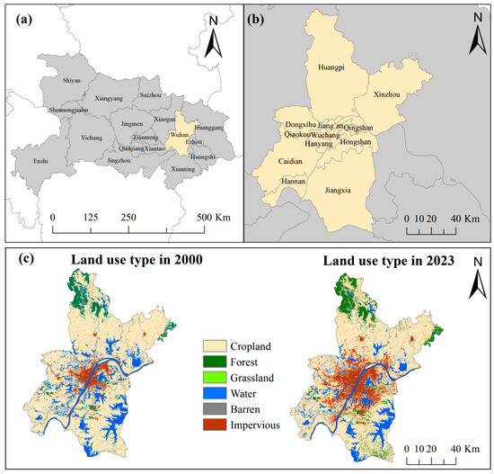
Figure 1.
Study area and spatial context of Wuhan, China. (a) Location of Wuhan within Hubei Province and surrounding regions. (b) Administrative districts of Wuhan. (c) Land-use/land-cover patterns in Wuhan in 2000 and 2023.
With rapid industrialization and urban expansion, Wuhan’s ecosystems have been under sustained anthropogenic pressure. Large areas of ecological land have been converted, and lake- and wetland-dominated landscapes have contracted substantially. Previous studies indicate that since the late 1980s, the lake area in Wuhan’s central urban districts has decreased by approximately 56.9% [35]. This long-term loss of ecological land has weakened ecosystem service provision and reduced the capacity of ecosystems to buffer and regulate external disturbances, thereby posing increasing challenges to urban ecological resilience [36,37].
2.2. Data Sources
The datasets include land-use, human activity, natural environmental conditions, and three-dimensional urban morphology. For datasets that are updated regularly (e.g., nighttime lights and CO2 emissions), we used the most recent releases consistent with the 2023 reference year. Detailed specifications and sources are summarized in Table 1.

Table 1.
Summary of the datasets used in this study.
Three-dimensional urban morphological variables were obtained from the 3D Global Building Footprint (3D-GloBFP) dataset, which provides globally consistent, building-level vector data describing urban 3D morphology for the 2020 reference year [42]. The 3D-GloBFP product was developed by integrating multi-source remote sensing features with derived morphological attributes compiled across multiple years. It therefore represents a temporally consistent snapshot of global building morphology for 2020 and does not provide annual updates for subsequent years. Using the 2020 snapshot is methodologically appropriate because key morphological attributes (e.g., building height and building volume) typically change gradually over short time horizons, and built environment effects on urban ecological processes often exhibit time-lagged responses [43,44].
In this study, we assessed ecological resilience for three benchmark years (2000, 2011, and 2023) to describe its long-term spatiotemporal evolution in Wuhan. The subsequent nonlinear analysis focused on the 2023 cross-section and examined the associations between built environment characteristics and the most recent ecological resilience outcomes.
To ensure spatial consistency across datasets, we first projected all raster layers to the WGS 1984 Albers equal-area coordinate system. Because the datasets have heterogeneous native resolutions, we resampled all raster variables to a common 1 km resolution. Categorical variables (e.g., land-use/land cover) were resampled using nearest-neighbor assignment to preserve class integrity. Continuous variables were resampled using bilinear interpolation to retain smooth spatial gradients while minimizing resampling artifacts. For vector datasets (e.g., road networks) and building-level morphology from 3D-GloBFP, we aggregated the original features onto the same 1 km × 1 km grid rather than interpolating.
A uniform 1 km × 1 km grid was used as the basic analytical unit to partition the study area, yielding 9005 grid cells across Wuhan. The ecological resilience index was calculated for each grid cell, and incomplete grids were excluded, yielding a final sample of 7440 valid grid cells.
3. Methods
3.1. Study Framework
As shown in Figure 2, this study followed a seven-step workflow to investigate the nonlinear associations between the built environment and urban ecological resilience at a 1 km grid scale. Step 1 constructed the Ecological Resilience Index (ERI) by integrating ecosystem resistance (Res), adaptability (Ada), and recovery capacity (Rec). Step 2 compiled built environment indicators encompassing human activity and urban morphology, as well as natural factors. Step 3 assessed spatial autocorrelation to quantify the spatial dependence in ERI. Step 4 performed variable preprocessing and implemented block-based spatial cross-validation strategies; specifically, 1 km grids were grouped into 10 km blocks with unique IDs, enabling spatially stratified splitting (GroupShuffleSplit) into training and test sets. Step 5 conducted Bayesian hyperparameter optimization for the XGBoost model using the Optuna (v4.4.0) framework, employing internal 5-fold GroupKFold spatial cross-validation within the training blocks. Step 6 trained the final model using the optimal hyperparameters, generated predictions for the testing set, and reported performance metrics (RMSE, R2, and MAE). Finally, Step 7 applied SHAP to interpret the model outputs, including feature importance, nonlinear response curves, and pairwise interaction patterns.
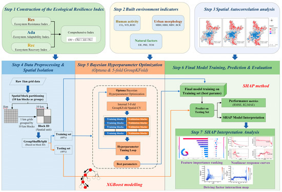
Figure 2.
Flow chart of the research framework.
3.2. Construction of the Ecological Resilience Index
Urban ecological resilience refers to the integrated capacity of ecosystems to maintain structural and functional stability, recover from disturbances, and adapt to environmental change. Following established assessment frameworks, we conceptualize ecological resilience as a multidimensional construct comprising resistance, adaptability, and recovery capacities [45,46,47]. To ensure comparability across indicators with heterogeneous units, we normalized each component to the [0, 1] range and then calculated the Urban Ecological Resilience Index (ERI) as the geometric mean of the three capacities. This multiplicative form reflects the premise that a deficiency in any single component can constrain overall resilience, consistent with prior index-based resilience assessments [10,48].
3.2.1. Ecosystem Resistance Index
Ecosystem resistance (Res) refers to the ability of urban ecosystems to absorb external disturbances, withstand environmental stressors, and maintain system stability. Prior studies suggest that resistance is closely linked to the provision of essential ecosystem services [49]. Accordingly, we selected five ecosystem service indicators: carbon storage, food production, biodiversity conservation, soil retention, and water yield. These indicators were quantified using the InVEST model [11,50]. We then constructed an integrated ecosystem services index to represent urban ecosystem resistance.
In this equation, ES denotes the composite ecosystem services index; fi represents the weight assigned to ecosystem service i (set to 0.2); and ESi denotes the normalized value of ecosystem service i.
3.2.2. Ecosystem Adaptability Index
Urban ecological adaptability (Ada) refers to the capacity of ecosystems to adjust their structures and functions in response to internal and external stressors, thereby reducing adverse impacts and supporting adaptive regulation and recovery processes [47]. The stability of landscape structure is closely correlated to the spatial organization and connectivity of landscape patterns, which reflect ecosystem heterogeneity and functional integrity [51,52]. Accordingly, we used landscape pattern indices to operationalize urban ecological adaptability through three dimensions: landscape heterogeneity, connectivity, and structure. Specifically, these dimensions were quantified using Shannon’s Diversity Index (SHDI), Shannon’s Evenness Index (SHEI), Interspersion and Juxtaposition Index (IJI), Contagion Index (CONTAG), Landscape Division Index (DIVISION), and Area-weighted Mean Fractal Dimension (FRAC_AM), as summarized in Table 2.
Table 2.
Landscape pattern indices.
Within this framework, ecological adaptability operationalized using three composite landscape attributes. Landscape heterogeneity (LH) captures the diversity and richness of landscape composition, reflecting structural complexity. Landscape connectivity (LC) describes the spatial continuity and functional linkages among landscape patches that enable ecological flows and species movement. Landscape structure (LS) characterizes the spatial organization and degree of fragmentation in landscape patterns, indicating the integrity and stability of ecosystem configuration.
The selected landscape pattern indices were computed using FRAGSTATS 4.3. Indicator weights were determined using a hybrid scheme that integrates the entropy weight method and the CRITIC method, capturing both information variability and inter-indicator contrast.
3.2.3. Ecosystem Recovery Index
Urban ecological recovery (Rec) refers to the ability of urban ecosystems to restore their structures and functions through self-regulation after natural or anthropogenic disturbances [46,47]. To quantify ecosystem recovery, this study adopted the land-use-based recovery model proposed by Peng et al. [52], with resistance and recovery weights set to 0.4 and 0.6, respectively. These weights reflect the extent to which each land-use type can withstand external disturbances and restore ecosystem health [53]. This index-based approach has been widely used in ecological resilience and ecosystem health assessments to represent relative recovery potential across heterogeneous landscapes [11,13,54].
where n denotes the number of land-use categories; Pi represents the proportion of area occupied by a given land-use category; and Recoi and Resisti denote the recovery and resistance coefficients associated with land-use type i, respectively. The specific values of these coefficients are summarized in Table 3. The resistance and recovery coefficients used in this study are empirical parameters derived from established land-use-based ecosystem resilience and health assessment literature. These coefficients are intended to represent relative differences in recovery potential and resistance capacity among land-use categories rather than exact recovery rates [11].
Table 3.
Ecosystem resilience coefficients for each landscape type.
Although the resistance (Res), adaptability (Ada), and recovery (Rec) are conceptually related, they are intended to capture distinct dimensions of urban ecosystems. Specifically, Res is measured using ecosystem-service indicators quantified with the InVEST model, which primarily represent functional outputs and biophysical processes. Ada is measured using landscape pattern metrics that emphasize spatial configuration, heterogeneity, and connectivity. Rec captures on land-use-based restoration potential. Accordingly, we treat these three components as complementary yet distinct dimensions in constructing ERI. To further examine potential redundancy among the three composites (Res, Ada, and Rec), we calculated variance inflation factors (VIFs). The VIFs were 1.03 (Res), 1.16 (Ada), and 1.14 (Rec), indicating negligible multicollinearity. This diagnostic supports interpreting Res, Ada, and Rec as complementary but empirically distinct components of ERI.
3.3. Selection of Built Environment Indicators
In line with the research objectives and data availability, we selected indicators to examine nonlinear associations between the built environment and urban ecological resilience. From an urban science perspective, the built environment is conceptualized as a multidimensional system that reflects how human activities are organized, concentrated, and physically manifested in urban space. It encompasses both anthropogenic activities and the spatial and morphological structures that serve as their physical carriers [11,14]. Accordingly, built environment indicators were grouped into two primary dimensions: human activity and urban morphological characteristics. Human activity indicators capture the magnitude and spatial concentration of socioeconomic pressures on urban ecosystems, whereas urban morphological indicators describe the built environment’s physical form, spatial configuration, and vertical structure [18,19]. In addition to built environment indicators, we incorporated natural environmental variables as background conditions rather than focal predictors. Climatic, topographic, and hydrological factors define the biophysical context in which urban development occurs and constrain ecosystem sensitivity and adaptive capacity. Including these background variables helps distinguish built environment associations from environmental constraints and supports a more comprehensive assessment of how built environment characteristics interact with natural conditions to shape urban ecological resilience [11].
3.3.1. Human Activity Indicators
Human activity captures the functional and socioeconomic dimensions of the built environment and reflects the magnitude of anthropogenic pressures on urban ecosystems. We used three indicators: CO2 emissions (CO2), nighttime light intensity (NTL), and road density (ROD) (Table 4). CO2 emissions serve as a proxy for the intensity of regional industrial development by reflecting energy consumption and the concentration of industrial activities. They also indicate potential ecosystem stress associated with production-related emissions and resource use [55,56]. Nighttime light intensity reflects urban infrastructure development, the concentration of commercial activities, and energy consumption, and it is therefore widely used as a proxy for regional economic vitality and anthropogenic activity intensity [57,58,59]. Road density measures the intensity of transportation infrastructure, which can reshape land-use patterns and contribute to habitat fragmentation, the diffusion of pollution, and increased human disturbance. Areas close to dense road networks are thus more likely to experience anthropogenic pressures that disrupt ecosystem connectivity and structure [60,61].
Table 4.
Summary of human activity indicators used in this study.
3.3.2. Urban Morphology Indicators
Urban morphology describes the physical and spatial form of the built environment and provides the structural basis through which human activities are embedded in urban space and interact with ecological processes. Based on prior empirical studies, four indicators were selected: building coverage ratio (BCR), mean building height (MBH), maximum building height (HBH), and mean building volume (MBV) [24,44,62]. Detailed definitions are provided in Table 5 and Figure 3. BCR measures the proportion of ground surface occupied by buildings within each 1 km grid cell and reflects horizontal built intensity [63]. MBH represents the overall level of vertical development, whereas HBH captures height extremes that may signal localized vertical intensification [22,44]. MBV represents three-dimensional built mass by combining building footprint and height information, providing a volumetric measure of built form [62,64]. All morphology indicators were computed at the 1 km grid scale.
Table 5.
Definition of urban morphology indicators used in this study.
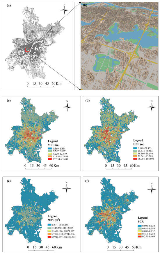
Figure 3.
Grid-based characterization of urban morphological features in Wuhan. (a) Spatial distribution of buildings in Wuhan. (b) 3D visualization of the urban built environment in a representative local area. (c) Mean building height (MBH). (d) Height of the tallest building (HBH). (e) Building volume (MBV). (f) Building coverage ratio (BCR).
3.3.3. Natural Environmental Indicators
Natural environmental conditions define the biophysical context in which the built environment operates and may modulate the associations between built environment characteristics and ecological resilience. Accordingly, we included elevation (ELE), precipitation (PRE), and air temperature (TEM) as background variables (Table 6) [65,66,67].
Table 6.
Summary of natural environmental indicators used in this study.
3.4. Spatial Autocorrelation Analysis
Global Moran’s I measures the overall degree of spatial autocorrelation and indicates whether urban ecological resilience is spatially clustered, dispersed, or randomly distributed across the study area. To identify localized clustering patterns, we applied univariate local Moran’s I (LISA) and classified grid cells into four types: high–high (HH), low–low (LL), high–low (HL), and low–high (LH). HH and LL indicate spatial clustering of similar resilience levels, whereas HL and LH represent spatial outliers [32,45].
Given the regular grid structure of the study area, we defined spatial relationships using Queen’s contiguity, treating grid cells sharing a common edge or corner as neighbors. This specification captures local interactions between adjacent urban units and is widely used in grid-based urban analyses [68,69,70]. The resulting spatial autocorrelation patterns were interpreted descriptively to characterize intra-urban spatial structure and to provide contextual support for subsequent machine-learning analyses.
3.5. Bayesian-Optimized XGBoost–SHAP Model
To account for the pronounced spatial dependence of ecological resilience, we adopted a block-based spatial cross-validation strategy for model calibration and evaluation. Because the data are gridded, spatial autocorrelation among adjacent cells can yield overly optimistic performance estimates if conventional random cross-validation is used [32,71].
Specifically, we aggregated 1 km grid cells into spatially contiguous blocks based on their projected centroid coordinates, and assigned all cells within each block a unique block ID. For an independent evaluation, we first split the dataset into spatial training (60%) and spatial testing (40%) sets by assigning entire blocks to either set using a block-based strategy [72]. The held-out test set was excluded from all subsequent model calibration and hyperparameter optimization. We determined the blocking scale via sensitivity analyses across candidate block sizes (5–20 km) and used the selected scale in the main experiments [73,74].
Model calibration was performed exclusively on the spatial training set using five-fold GroupKFold cross-validation, where folds were defined by spatial block membership rather than random sampling. Although each 1 km grid cell was treated as an individual observation, cross-validation was conducted at the block level to maintain spatial independence between training and validation folds. Bayesian hyperparameter optimization was performed using the Tree-structured Parzen Estimator (TPE) algorithm implemented in Optuna [23,24,75,76,77]. Hyperparameter tuning was conducted entirely within the training set via the same five-fold spatial cross-validation, ensuring that parameter selection relied on spatially independent validation results. Compared with conventional random cross-validation, this spatially explicit strategy provides a more conservative and realistic estimate of model performance under spatial heterogeneity.
After identifying the optimal hyperparameter configuration, we retrained the final XGBoost model on the full spatial training set and evaluated it on the spatially independent test set. Model performance was quantified using the coefficient of determination (R2), mean squared error (MSE), root mean squared error (RMSE), and mean absolute error (MAE) [24].
In these equations, denotes the observed value of the i-th sample, denotes the corresponding model-predicted value, refers to the mean of all observed values, and n denotes the total number of samples.
To improve the interpretability of the machine-learning results, we used the Shapley Additive Explanations (SHAP) framework, grounded in cooperative game theory, to quantify each predictor’s contribution to ERI [78]. SHAP values were computed as follows:
where ϕᵢ denotes the Shapley value associated with feature i, representing its marginal contribution to ERI prediction. N d denotes the full set of input features, and S represents any subset of features excluding feature i. The total number of features is denoted by n. The function v(S) corresponds to the model output using only the features in subset S, whereas v(S∪{i}) represents the predicted outcome after incorporating feature i.
4. Results
4.1. Analysis of Land-Use Change
As shown in Figure 4 and Table 7, Wuhan’s land-use structure changed substantially between 2000 and 2023. Overall, the period was characterized by rapid expansion of built-up land, sustained declines in cropland and water bodies, and a gradual increase in forest land. Cropland decreased from 6238.65 km2 in 2000 to 5552.42 km2 in 2023, a net loss of 686.23 km2, representing the largest absolute reduction among all land-use types. Water bodies declined from 1303.58 km2 to 1098.50 km2, a net decrease of 205.09 km2. In contrast, forest land increased from 509.10 km2 to 666.02 km2, a net gain of 156.92 km2. Built-up land exhibited the most pronounced expansion, increasing from 525.76 km2 to 1263.18 km2, for a net increase of 737.42 km2.
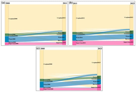
Figure 4.
Land-use transitions in Wuhan. (a) 2000–2011. (b) 2011–2023. (c) 2000–2023.
Table 7.
Land-use transfer matrix for Wuhan from 2000 to 2023 (km2).
Regarding land-use transitions (Table 7), cropland exhibited the most extensive conversion to other categories, primarily to built-up land, water bodies, and forest land. Among these transitions, the conversion from cropland to built-up land totaled 674.63 km2, representing the largest contribution to built-up land inflows and the dominant pathway of urban expansion. Conversions from water bodies to cropland and to built-up land were also evident, amounting to 285.61 km2 and 69.01 km2, respectively. Transitions between forest land and grassland occurred at relatively small scales; nonetheless, forest land showed an overall net gain.
4.2. Spatiotemporal Variation and Clustering of ERI
Figure 5 shows the temporal evolution of the three ecological resilience subdimensions in Wuhan from 2000 to 2023. Overall, ecological adaptability remained relatively stable, with only minor fluctuations over time. In contrast, ecological recovery exhibited a sustained decline. Ecological resistance decreased initially and then rebounded in the later period.
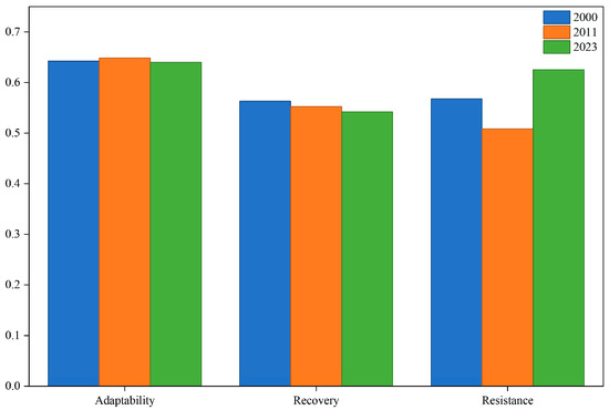
Figure 5.
Temporal and spatial changes in the ecological resilience at the subsystem level.
Figure 6 presents the ERI classification and its spatiotemporal patterns in Wuhan. Using the Jenks natural breaks method, ERI was classified into five levels: weak (0 < ERI ≤ 0.4276), relatively weak (0.4277 < ERI ≤ 0.5364), moderate (0.5365 < ERI ≤ 0.6104), relatively good (0.6105 < ERI ≤ 0.6726), and good (ERI > 0.6727). Temporally, the share of areas classified as weak or relatively weak increased markedly from 2000 to 2011, whereas the shares of relatively good and good classes rebounded from 2011 to 2023. Spatially, central districts (e.g., Jiang’an, Jianghan, Qiaokou, Wuchang, and Hongshan) exhibited comparatively lower ERI, while peripheral districts (e.g., Huangpi, Xinzhou, Jiangxia, and Caidian) showed higher overall ERI.
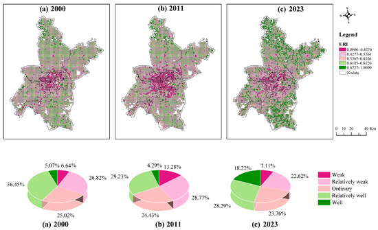
Figure 6.
Spatial-temporal change in ERI. (a) 2000. (b) 2011. (c) 2023.
Figure 7 shows significant and persistent positive spatial autocorrelation of urban ecosystem resilience in 2000, 2011, and 2023. Global Moran’s I values were 0.5197, 0.5951, and 0.5945, respectively, and all were positive and statistically significant (p ≤ 0.001). The LISA maps further revealed clear high–high (HH) and low–low (LL) clusters, indicating pronounced intra-urban spatial heterogeneity. HH clusters were mainly concentrated in the forest-rich northern, northeastern, and southeastern peripheral areas, whereas LL clusters were primarily located in the central built-up area. In 2023, we identified 1818 HH cells and 1538 LL cells; in contrast, spatial outliers were rare, with only 124 high–low (HL) and 44 low–high (LH) cells.
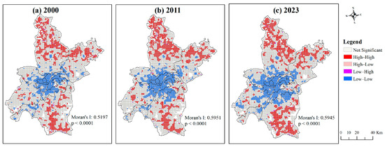
Figure 7.
LISA maps and Global Moran’s I values of ERI. (a) 2000. (b) 2011. (c) 2023.
4.3. Correlation Analysis and Multicollinearity Diagnostics
We examined intercorrelations among the predictors using Pearson correlation analysis (Figure 8) and assessed potential multicollinearity using variance inflation factors (VIFs) (Table S1). Most variable pairs had absolute correlation coefficients below 0.80. In addition, all predictors had VIF values below 10, indicating that severe multicollinearity was unlikely.
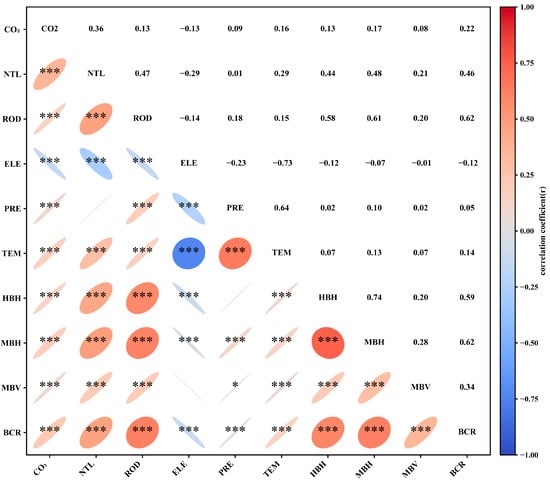
Figure 8.
Pearson correlation analysis among variables. * p < 0.05; ** p < 0.01; *** p < 0.001.
4.4. Key Predictors Identified by XGBoost
Model implementation and parameter optimization were conducted in Python 3.9. XGBoost (v2.0.3) was used as the core learning algorithm, Optuna (v4.4.0) was used for Bayesian hyperparameter optimization, and SHAP (v0.47.0) was used to interpret model predictions. Hyperparameter search ranges and the corresponding optimal configurations under different spatial blocking scales are summarized in Table 8.
Table 8.
Optimal parameter settings of the Bayesian-optimized XGBoost.
Model performance was evaluated using four standard metrics, including mean squared error (MSE), root mean squared error (RMSE), mean absolute error (MAE), and the coefficient of determination (R2), as reported in Table 9. To avoid overly optimistic performance estimates driven by spatial autocorrelation, we employed a block-based spatial validation strategy that assigns entire spatial blocks to either the training or testing set. The blocking scale was selected through a sensitivity analysis across candidate block sizes (5, 10, 15, and 20 km) while keeping the modeling and optimization workflow unchanged. Test performance was comparable under 5–10 km blocking (R2 ≈ 0.50), but declined markedly at coarser scales (R2 = 0.39 at 15 km and 0.22 at 20 km), suggesting that overly coarse blocking reduces the effective number of spatially independent training groups and poses a more stringent cross-block generalization task. Based on this robustness check, we adopted 10 km blocks for the main analyses. Under this setting, the Bayesian-optimized XGBoost model achieved R2 = 0.6091 on the training set and 0.5014 on the spatially independent test set, with corresponding RMSE values of 0.06024 and 0.06759, respectively. For completeness, results from conventional random cross-validation are reported in the Supplementary Materials. As expected, random cross-validation yields more optimistic performance estimates than spatially blocked evaluation.
Table 9.
Model performance of Bayesian-optimized XGBoost.
According to the XGBoost feature importance results (Figure 9a), BCR exhibited the largest substantial contribution to the model-predicted ERI, followed by NTL, ELE, MBH, PRE, and TEM. In the SHAP summary plot (Figure 9b), each point represents a 1 km grid cell; the x-axis position indicates the magnitude and direction of the SHAP value, and the color encodes the corresponding feature value.
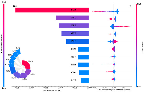
Figure 9.
Relative importance of explanatory variables in the XGBoost model. (a) Feature importance ranking. (b) SHAP summary plot.
BCR made the largest contribution to the model output (30.8%) and was predominantly distributed on the negative side of the SHAP axis, with higher BCR values generally corresponding to more negative SHAP values. NTL contributed 13.9%, with a similar distribution: higher values were mostly associated with negative SHAP values, and lower values clustered near zero. ELE accounted for 12.7% of the total contribution. MBH contributed 11.6%, with relatively higher positive SHAP values concentrated at intermediate building heights. PRE accounted for 9.6% and exhibited a non-monotonic SHAP pattern, clustering primarily at intermediate precipitation levels, with negative values at both low and high precipitation levels. TEM contributed 4.7%, with SHAP values tightly clustered around zero, indicating a minimal contribution to the model output.
As an additional robustness check, we replaced nighttime light intensity (NTL) with population density (POP) as an alternative proxy for human activity intensity, while maintaining the 10 km spatial blocking protocol and unchanged modeling workflow. The POP-substituted model produced comparable spatial test performance (test R2 = 0.5080, RMSE = 0.06714) to the baseline NTL model (test R2 = 0.5014, RMSE = 0.06759), and the SHAP-based interpretation remained consistent with the original mechanism.
4.5. Nonlinear Main Effects Revealed by SHAP
Figure 10 presents SHAP partial dependence plots for selected indicators, illustrating how their contributions to the ERI vary across the observed value ranges. The marked intersection points indicate changes in the relative position of SHAP values along the x-axis and are interpreted as descriptive features of the response curves rather than fixed breakpoints.
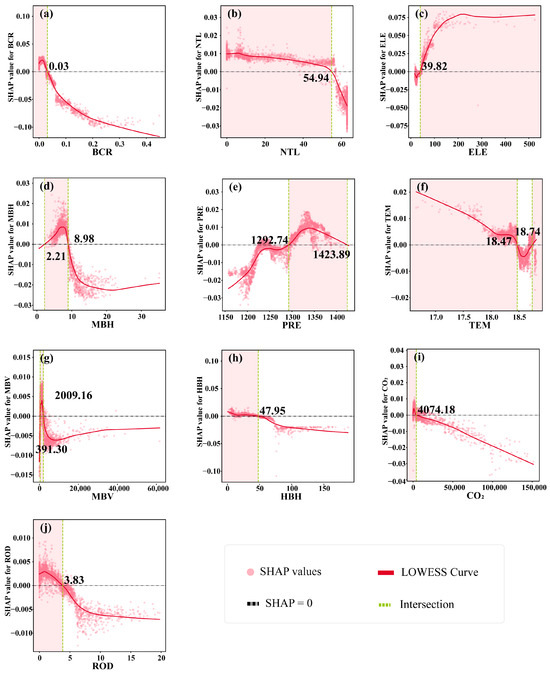
Figure 10.
Nonlinear and threshold effects of ERI drivers revealed by SHAP analysis. (a) BCR; (b) NTL; (c) ELE; (d) MBH; (e) PRE; (f) TEM; (g) MBV; (h) HBH; (i) CO2; (j) ROD. Each panel shows the SHAP dependence plot with the LOWESS trend line and the identified turning region (intersection).
For BCR, values below approximately 0.03 were associated with positive contributions to ERI, whereas higher values were associated with negative contributions. NTL showed positive contributions at lower levels, but the contribution turned negative as values exceeded about 54.94. ELE showed a negative contribution at lower elevations and a positive contribution at higher elevations, with a transition around 39.82 m. MBH showed positive contributions to predicted urban ecological resilience mainly between about 2.21 m and 8.98 m, whereas values below or above this interval were associated with negative contributions. PRE showed negative contributions below about 1292.74 mm, positive contributions between about 1292.74 mm and 1423.89 mm, and negative contributions again at higher levels. TEM presented a localized reduction in contribution around 18.47–18.74 °C. MBV showed negative contributions as values exceeded about 391.30 m3. HBH exhibited negative contributions at values above about 47.95 m. CO2 emissions, as an indicator of industrial development intensity, showed negative contributions beyond about 40,741.18 t·km−2·yr−1. ROD showed positive contributions at lower values but negative contributions above about 3.83 km·km−2.
4.6. SHAP Interaction Effects Among Built Environment Drivers
We used SHAP interaction values to quantify pairwise joint contributions of predictors to ERI. Figure 11 shows scatter plots for the six predictor pairs with the largest SHAP interaction values, illustrating how interaction contributions vary across the observed ranges of the two variables.
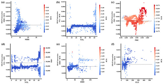
Figure 11.
Scatter plot of SHAP interaction between characteristics (top 6). (a) MBH × BCR. (b) NTL × BCR. (c) PRE × TEM. (d) NTL × MBV. (e) HBH × BCR. (f) ELE × BCR. Point colors indicate the value of the second feature in each interaction pair.
Regarding urban morphology, under high BCR, interaction contributions were more often positive when HBH exceeded approximately 50 m or when MBH is below approximately 10 m. A similar pattern was observed at lower elevations (ELE < 50 m): high BCR was associated with positive interaction contributions, whereas low BCR was associated with negative contributions. Regarding human activity, when NTL is above approximately 50, interaction contributions varied with MBV: high NTL combined with high MBV was mainly associated with positive interaction values, whereas high NTL combined with low MBV or with low BCR was mainly associated with negative interaction values. For the PRE × TEM interaction, when PRE exceeded approximately 1300 mm, lower TEM co-occurred with predominantly negative SHAP interaction values.
5. Discussion
5.1. Nonlinear and Threshold Effects of Built Environment Indicators on the ERI
The XGBoost results suggest that human activity indicators are generally associated with negative contributions to the model-predicted urban ecological resilience. This pattern is consistent with ecological theory, which posits that intensified human activities (e.g., industrial development and urban expansion) can place sustained pressures on ecosystems by reshaping land-use patterns and increasing resource consumption [11,79]. In line with these model-derived associations, previous studies have reported that such pressures often coincide with ecological fragmentation and disruptions to ecological processes, which may undermine structural integrity and reduce the capacity to sustain ecosystem functions [80,81].
From an urban-form perspective, BCR in Wuhan showed a positive SHAP contribution to the predicted ERI when BCR was below approximately 3%; as the BCR increased, the contribution shifted from positive to negative. This nonlinear pattern is consistent with prior research suggesting that high building coverage can intensify surface sealing, thereby limiting rainfall infiltration and soil-moisture replenishment, and can also impede natural airflow within dense building clusters [82,83,84]. The model-inferred turning region is further supported by Yang et al., who reported that high-density built-up patterns tend to reduce neighborhood-scale air exchange efficiency and increase thermal stress, potentially compromising ecological resilience [85]. These values should be interpreted as turning regions in the SHAP response curves at the 1 km grid scale rather than universal cutoffs for site-level regulation.
Additionally, MBH exhibited an inverted U-shaped relationship with the predicted ERI, with positive contributions concentrated in the range of approximately 2.21–8.98 m. This interval is derived from 1 km grid-mean values and should not be interpreted as a rigid constraint on individual buildings. Rather, it may reflect areas with moderate development intensity that tend to co-occur with higher shares of blue–green infrastructure, where shading and evapotranspiration can reduce thermal loads, and where building geometry and height configuration can influence street-canyon ventilation and radiative exchange [86].
5.2. SHAP Interaction Effects Among Built Environment Indicators on the ERI
Beyond individual predictors, SHAP interaction analysis suggests that under high BCR, interaction contributions are more often positive when HBH exceeds approximately 50 m or when MBH is below approximately 10 m. Importantly, these interaction patterns are conditional on BCR and should not be interpreted as evidence that high density is universally beneficial. Previous studies suggest that, compared with dispersed outward expansion, more compact and concentrated development may, in some scenarios, reduce additional fragmentation of remaining ecological space and help maintain ecological patch connectivity [87,88]. However, any potential benefits are likely context dependent and may be constrained by local conditions, including ventilation, the thermal environment, and stormwater capacity [24,89].
The NTL × MBV interaction suggests two distinct patterns in the model. When NTL was high but MBV was low, interaction contributions were generally negative. This pattern may reflect areas with high activity intensity but limited vertical built mass, where constrained ventilation can promote the accumulation of heat and pollutants; moreover, higher NTL may also capture pressures related to energy consumption and light pollution [90,91]. In contrast, when both NTL and MBV were high, interaction contributions tended to be positive. This model-derived pattern may correspond to vertically intensified and functionally concentrated development, in which additional floor space can be achieved with a relatively small marginal increase in surface occupation [89]. Wu et al. further reported that, in high-density built-up areas, the structural configuration and connectivity of green infrastructure are closely linked to resilience performance, which provides contextual support for this interpretation [92].
Finally, this study focused on Wuhan, China; therefore, the observed relationships between urban morphology and predicted ERI, including nonlinear responses and threshold patterns, may not be directly generalizable to cities with different geographic, climatic, or morphological contexts.
5.3. Implications for Urban Planning and Management
Given Wuhan’s concurrent needs for ecological conservation and development, urban planning should shift from predominantly restrictive control toward proactive guidance through optimizing the allocation of spatial resources to achieve synergistic improvements in development outcomes and ecological resilience. The planning permit process can serve as a key entry point for strengthening microenvironmental governance. As a major economic, scientific, and educational hub, Wuhan should pay particular attention to microenvironmental impacts in high-intensity development areas. Planning policies can steer both new and existing construction land toward functional mixing and vertical intensification. In high-intensity areas, requirements such as ventilation corridor protection and three-dimensional ecological measures, such as green roofs and vertical greening, can be incorporated into planning standards. During environmental impact assessment and planning approval, technical reviews can be strengthened for building massing, blue–green space configuration, and microenvironmental design. Policy instruments such as FAR incentives can be used to set conditions for high-intensity development, including requirements for contiguous green-space provision, the creation of elevated ventilation layers, and compliance with vertical-greening targets. In addition, ventilation assessment reports based on simulation analysis and dedicated design submissions for three-dimensional ecological measures can be required as part of the technical review and acceptance procedures for major projects in designated areas.
Furthermore, Wuhan’s dense river network and low-lying topography may increase ecological vulnerability in certain areas. Planning management should curb encroachment on lakes, wetlands, and flood-conveyance corridors and strengthen enforcement of ecological protection red lines. In ecologically sensitive, flood-prone, low-lying areas, planning priorities should shift from conventional land development toward nature-based solutions. Urban renewal and infrastructure projects can prioritize hybrid green–gray measures (e.g., rain gardens and constructed wetlands) and embed long-term operation and maintenance responsibilities, together with dedicated budget commitments, into municipal management programs.
These planning implications are intended to be indicative rather than prescriptive and should be applied cautiously, with due consideration of local governance capacity, data uncertainty, and site-specific ecological conditions.
5.4. Limitations and Future Work
Despite providing systematic insights into the spatial patterns and potential drivers of ecological resilience in high-density cities, as illustrated by the Wuhan case, this study has several limitations that warrant further investigation in future research.
First, previous studies have noted that grid-based partitioning may fragment the urban fabrics and obscure fine-scale morphological heterogeneity, and have therefore recommended block-based units for analyzing micro-scale processes such as land surface temperature [93,94]. Future research could extend our framework by adopting block-based or functional-zone units. Integrating block-level morphology with ecological resilience assessment across multiple spatial scales is a promising direction for improving understanding of scale-dependent built environment–resilience relationships [95,96,97].
Second, the availability of comprehensive three-dimensional urban morphology data is often limited to a few reference years. As a result, our nonlinear analyses relied primarily on cross-sectional data, which constrained our ability to examine temporal dynamics and the nonlinear evolution of urban ecological resilience. Future research could address this limitation by incorporating multi-temporal 3D urban morphology products or long-term remote sensing datasets to enable dynamic, time-aware nonlinear analyses of ecological resilience [43,82]. Moreover, although block-based spatial cross-validation was used to reduce spatial dependence, this study remains a single-city case. We also did not conduct stratified subregional validation (e.g., comparing central versus suburban areas or differentiating zones by proximity to major water bodies); therefore, the reported nonlinear patterns should be interpreted as city- and scale-specific associations. Future research could test model transferability by incorporating stratified validation across multiple cities or regions with heterogeneous development contexts, and across intra-urban subregions or functional zones [98,99].
Finally, although the XGBoost–SHAP framework is effective for identifying nonlinear relationships, threshold-like patterns, and interactions, it is fundamentally data driven and does not explicitly establish causal mechanisms. Therefore, the reported relationships should be interpreted as model-based associations rather than direct causal evidence. Future research could combine this framework with causal inference approaches, such as quasi-experimental designs, longitudinal analyses, and structural equation modeling, as well as process-oriented methods (e.g., system dynamics), to better disentangle the mechanisms shaping urban ecological resilience [100,101,102].
6. Conclusions
This study integrates multi-source data to examine nonlinear associations between the built environment and ecological resilience in a high-density city using Wuhan, China, as a case study. We employed a Bayesian-optimized XGBoost–SHAP framework with block-based spatial cross-validation to reduce spatial leakage and provide a more conservative performance assessment under spatial dependence. The main findings are summarized as follows.
First, land-use transitions in Wuhan from 2000 to 2023 were characterized by rapid expansion of built-up land, continued declines in cropland and water bodies, and a moderate increase in forest land. Urban ecological resilience showed a gradual improvement in recent years. Global and local Moran’s I indicated significant spatial autocorrelation, with high–high clusters concentrated in the forest-rich northern, northeastern, and southeastern periphery and low–low clusters primarily located in the central built-up area.
Second, the Bayesian-optimized XGBoost–SHAP framework identified nonlinear thresholds via spatial-block-based cross-validation, achieving an R2 of 0.5014 on a spatially independent test set. Feature-importance and SHAP results indicated that BCR was the most influential predictor (30.8%), followed by NTL, ELE, and MBH.
Third, several built environment indicators exhibited clear threshold-like patterns. Higher BCR and NTL values beyond the identified turning regions were associated with more negative SHAP contributions to ERI (BCR > 0.03; NTL > 54.94). By contrast, MBH showed an inverted U-shaped pattern, with positive contributions concentrated between 2.21 and 8.98 m.
Finally, SHAP interaction analysis suggested that, under high BCR, interactions with HBH > 50 m, MBH < 10 m, or ELE < 50 m were predominantly positive. Likewise, the interaction between high NTL (>50) and high MBV was mainly positive, whereas high PRE (>1300 mm) combined with lower TEM was associated with predominantly negative interaction contributions.
7. Patents
There are no patents resulting from the work reported in this manuscript.
Supplementary Materials
The following supporting information can be downloaded at: https://www.mdpi.com/article/10.3390/buildings16040844/s1, Table S1. VIF for Indicators; Table S2. Descriptive statistics of indicators; Table S3. Optimal hyperparameters of the Bayesian-optimized XGBoost (spatial blocking CV vs. random split CV); Table S4. Predictive performance of the Bayesian-optimized XGBoost (spatial blocking CV vs. random split CV); Table S5. Optimal hyperparameters of the Bayesian-optimized XGBoost (POP replacing NTL); Table S6. Alternative-indicator robustness check (POP replacing NTL); Table S7. VIF for resistance (Res), adaptability (Ada), and recovery (Rec); Figure S1. Relative importance of explanatory variables in the XGBoost model (POP replacing NTL); Figure S2. Nonlinear and threshold effects of ERI drivers revealed by SHAP analysis (POP replacing NTL); Figure S3. Pairwise Pearson correlations between resistance (Res), adaptability (Ada), and recovery (Rec).
Author Contributions
K.F.: writing—original draft, visualization, methodology, conceptualization; J.W.: writing—review and editing, resources, methodology, funding acquisition; Y.H.: software, investigation, data curation; All authors have read and agreed to the published version of the manuscript.
Funding
This research was supported by the Yunnan Provincial Philosophy and Social Sciences Project (Grant No. ZX2024YB46).
Data Availability Statement
Data will be made available on request.
Acknowledgments
The authors have reviewed and edited the output and take full responsibility for the content of this publication.
Conflicts of Interest
J.W. received funding from the Yunnan Provincial Philosophy and Social Sciences Project, which supported the data collection and analysis. The funders had no influence on the interpretation of results or the decision to publish the manuscript. The authors declare no other conflicts of interest.
Abbreviations
The following abbreviations are used in this manuscript:
| Abbreviation | Definition |
| ERI | Ecological Resilience Index |
| Res | Ecosystem Resistance |
| Ada | Ecosystem Adaptability |
| Rec | Ecosystem Recovery |
| ES | Ecosystem Services |
| SHAP | SHapley Additive exPlanations |
| XGBoost | Extreme Gradient Boosting |
| CO2 | Carbon dioxide emissions |
| NTL | Nighttime light intensity |
| ROD | Road density |
| MBH | Mean building height |
| HBH | Maximum building height |
| MBV | Mean building volume |
| BCR | Building coverage ratio |
| ELE | Elevation |
| PRE | Precipitation |
| TEM | Air temperature |
| SHDI | Shannon’s diversity index |
| SHEI | Shannon’s evenness index |
| IJI | Interspersion and juxtaposition index |
| CONTAG | Contagion index |
| DIVISION | Landscape division index |
| FRAC_AM | Area-weighted mean fractal dimension |
References
- Adger, W.N.; Hughes, T.P.; Folke, C.; Carpenter, S.R.; Rockström, J. Social-Ecological Resilience to Coastal Disasters. Science 2005, 309, 1036–1039. [Google Scholar] [CrossRef]
- Holling, C.S. Resilience and Stability of Ecological Systems. Annu. Rev. Ecol. Evol. Syst. 1973, 4, 1–23. [Google Scholar] [CrossRef]
- Xiao, W.; Lv, X.; Zhao, Y.; Sun, H.; Li, J. Ecological Resilience Assessment of an Arid Coal Mining Area Using Index of Entropy and Linear Weighted Analysis: A Case Study of Shendong Coalfield, China. Ecol. Indic. 2020, 109, 105843. [Google Scholar] [CrossRef]
- Reid, W.V.; Mooney, H.A. The Millennium Ecosystem Assessment: Testing the Limits of Interdisciplinary and Multi-Scale Science. Curr. Opin. Environ. Sustain. 2016, 19, 40–46. [Google Scholar] [CrossRef]
- Kephart, J.L.; Sánchez, B.N.; Moore, J.; Schinasi, L.H.; Bakhtsiyarava, M.; Ju, Y.; Gouveia, N.; Caiaffa, W.T.; Dronova, I.; Arunachalam, S.; et al. City-Level Impact of Extreme Temperatures and Mortality in Latin America. Nat. Med. 2022, 28, 1700–1705. [Google Scholar] [CrossRef]
- Uttajug, A.; Seposo, X.; Phosri, A.; Phung, V.L.H.; Tajudin, M.A.B.A.; Ueda, K. Effects of Coexposure to Air Pollution from Vegetation Fires and Extreme Heat on Mortality in Upper Northern Thailand. Environ. Sci. Technol. 2024, 58, 9945–9953. [Google Scholar] [CrossRef]
- Retallack, M. The Intersection of Economic Demand for Ecosystem Services and Public Policy: A Watershed Case Study Exploring Implications for Social-Ecological Resilience. Ecosyst. Serv. 2021, 50, 101322. [Google Scholar] [CrossRef]
- Suding, K.; Higgs, E.; Palmer, M.; Callicott, J.B.; Anderson, C.B.; Baker, M.; Gutrich, J.J.; Hondula, K.L.; LaFevor, M.C.; Larson, B.M.H.; et al. Committing to Ecological Restoration. Science 2015, 348, 638–640. [Google Scholar] [CrossRef]
- Yue, C.; Xu, M.; Ciais, P.; Tao, S.; Shen, H.; Chang, J.; Li, W.; Deng, L.; He, J.; Leng, Y.; et al. Contributions of Ecological Restoration Policies to China’s Land Carbon Balance. Nat. Commun. 2024, 15, 9708. [Google Scholar] [CrossRef]
- Ouyang, X.; Chen, J.; Wei, X.; Li, J. Ecological Resilience in China’s Ten Urban Agglomerations: Evolution and Influence under the Background of Carbon Neutrality. Ecol. Model. 2025, 508, 111226. [Google Scholar] [CrossRef]
- Chen, J.; Lei, F.; Zeng, H.; Xie, L.; Ouyang, X. Estimating Non-Linear Effects of Natural and Anthropogenic Factors on Ecological Resilience: Evidence from the Southern Hilly Areas. In Environment, Development and Sustainability; Springer: Berlin/Heidelberg, Germany, 2024. [Google Scholar] [CrossRef]
- Alberti, M.; Marzluff, J.M.; Shulenberger, E.; Bradley, G.; Ryan, C.; Zumbrunnen, C. Integrating Humans into Ecology: Opportunities and Challenges for Studying Urban Ecosystems. In Urban Ecology; Marzluff, J.M., Shulenberger, E., Endlicher, W., Alberti, M., Bradley, G., Ryan, C., Simon, U., ZumBrunnen, C., Eds.; Springer: Boston, MA, USA, 2008; pp. 143–158. [Google Scholar]
- Ma, X.; Zhang, J.; Wang, P.; Zhou, L.; Sun, Y. Estimating the Nonlinear Response of Landscape Patterns to Ecological Resilience Using a Random Forest Algorithm: Evidence from the Yangtze River Delta. Ecol. Indic. 2023, 153, 110409. [Google Scholar] [CrossRef]
- Eldesoky, A.H.; Abdeldayem, W.S. Disentangling the Relationship between Urban Form and Urban Resilience: A Systematic Literature Review. Urban Sci. 2023, 7, 93. [Google Scholar] [CrossRef]
- Feng, X.; Xiu, C.; Bai, L.; Zhong, Y.; Wei, Y. Comprehensive Evaluation of Urban Resilience Based on the Perspective of Landscape Pattern: A Case Study of Shenyang City. Cities 2020, 104, 102722. [Google Scholar] [CrossRef]
- Palazzo, E. Bridging Urban Morphology and Urban Ecology: A Framework to Identify Morpho-Ecological Periods and Patterns in the Urban Ecosystem. J. Urban Ecol. 2022, 8, juac007. [Google Scholar] [CrossRef]
- Zhang, C.; Zhou, Y.; Yin, S. Interaction Mechanisms of Urban Ecosystem Resilience Based on Pressure-State-Response Framework: A Case Study of the Yangtze River Delta. Ecol. Indic. 2024, 166, 112263. [Google Scholar] [CrossRef]
- Huang, Y.; Wang, Z.; Zhao, H.; You, D.; Peng, Y. Quantifying the Nonlinear Effects of Urban Morphological Features on Ecological Resilience: Evidence from Cities in China. Sustain. Cities Soc. 2026, 136, 107072. [Google Scholar] [CrossRef]
- Chen, Y.; Ma, W.; Shao, Y.; Wang, N.; Yu, Z.; Li, H.; Hu, Q. The Impacts and Thresholds Detection of 2D/3D Urban Morphology on the Heat Island Effects at the Functional Zone in Megacity during Heatwave Event. Sustain. Cities Soc. 2025, 118, 106002. [Google Scholar] [CrossRef]
- Li, J.; Zhang, Y.; Yang, L.; Shan, Z. Seasonal Variations in Ecological Environment Quality across Different Geomorphological Regions and Their Response Mechanisms to Climate Change. Sci. Rep. 2025, 15, 26385. [Google Scholar] [CrossRef]
- Qiao, R.; Wu, T.; Zhao, Z.; Gao, S.; Yang, T.; Duan, C.; Zhou, S.; Liu, X.; Xia, L.; Meng, X.; et al. Dissecting the Natural and Human Drivers of Urban Thermal Resilience across Climates. Geogr. Sustain. 2025, 6, 100255. [Google Scholar] [CrossRef]
- Tang, G.; Du, X.; Wang, S. Impact Mechanisms of 2D and 3D Spatial Morphologies on Urban Thermal Environment in High-Density Urban Blocks: A Case Study of Beijing’s Core Area. Sustain. Cities Soc. 2025, 123, 106285. [Google Scholar] [CrossRef]
- Lin, X.; Wang, Z.; Bao, Y.; Chen, X. Enhancing Urban Thermal Resilience in Multi-Mountainous Cities through Optimized 3D Block Morphology: A Machine Learning Framework. Energy Build. 2025, 349, 116562. [Google Scholar] [CrossRef]
- Wang, W.; Wang, Y.; Shen, C. Quantifying the Nonlinear and Interactive Effects of Urban Form on Resilience to Extreme Precipitation: Evidence from 192 Cities of Southern China. Sustain. Cities Soc. 2025, 125, 106366. [Google Scholar] [CrossRef]
- Wu, N.; Zhou, Y.; Yin, S.; Gong, H.; Zhang, C. Revealing the Nonlinear Impact of Environmental Regulation on Ecological Resilience Using the XGBoost-SHAP Model: Evidence from the Yangtze River Delta Region, China. J. Clean. Prod. 2025, 514, 145700. [Google Scholar] [CrossRef]
- Cao, Q.; Huang, H.; Hong, Y.; Huang, X.; Wang, S.; Wang, L.; Wang, L. Modeling Intra-Urban Differences in Thermal Environments and Heat Stress Based on Local Climate Zones in Central Wuhan. Build. Environ. 2022, 225, 109625. [Google Scholar] [CrossRef]
- Liu, L.; Wu, J. Scenario Analysis in Urban Ecosystem Services Research: Progress, Prospects, and Implications for Urban Planning and Management. Landsc. Urban Plan. 2022, 224, 104433. [Google Scholar] [CrossRef]
- Han, P.; Hu, H.; Zhou, J.; Wang, M.; Zhou, Z. Integrating Key Ecosystem Services to Study the Spatio-Temporal Dynamics and Determinants of Ecosystem Health in Wuhan’s Central Urban Area. Ecol. Indic. 2024, 166, 112352. [Google Scholar] [CrossRef]
- Lu, Y.; Liu, Y.; He, H.; Chen, F.; Wang, L.; Liu, Y. Diagnosing Degradation Risks of Ecosystem Services in Wuhan, China from the Perspective of Land Development: Identification, Measurement and Regulation. Ecol. Indic. 2022, 136, 108580. [Google Scholar] [CrossRef]
- Tan, C.; Xu, B.; Hong, G.; Wu, X. Integrating Habitat Risk and Landscape Resilience in Forest Protection and Restoration Planning for Biodiversity Conservation. Landsc. Urban Plan. 2024, 248, 105111. [Google Scholar] [CrossRef]
- Wang, B.; Wang, Y.; Wu, X. Impact of Land Use Compactness on the Habitat Services from Green Infrastructure in Wuhan, China. Urban For. Urban Green. 2023, 84, 127927. [Google Scholar] [CrossRef]
- Davtalab, M.; Byčenkienė, S. Synergistic Effects of Spatial Urban Form on PM2.5 Concentration and Urban Heat Islands: A Multi-Scale Explanatory Machine Learning. J. Clean. Prod. 2026, 538, 147226. [Google Scholar] [CrossRef]
- Roberts, D.R.; Bahn, V.; Ciuti, S.; Boyce, M.S.; Elith, J.; Guillera-Arroita, G.; Hauenstein, S.; Lahoz-Monfort, J.J.; Schröder, B.; Thuiller, W.; et al. Cross-validation Strategies for Data with Temporal, Spatial, Hierarchical, or Phylogenetic Structure. Ecography 2017, 40, 913–929. [Google Scholar] [CrossRef]
- Wang, Y.; Khodadadzadeh, M.; Zurita-Milla, R. Spatial+: A New Cross-Validation Method to Evaluate Geospatial Machine Learning Models. Int. J. Appl. Earth Obs. Geoinf. 2023, 121, 103364. [Google Scholar] [CrossRef]
- Xie, Q.; Liu, J. Spatio-Temporal Dynamics of Lake Distribution and Their Impact on Ecosystem Service Values in Wuhan Urbanized Area during 1987–2016. Acta Ecol. Sin. 2020, 40, 7840–7850. [Google Scholar] [CrossRef]
- Xiao, S.; Zou, L.; Xia, J.; Dong, Y.; Yang, Z.; Yao, T. Assessment of the Urban Waterlogging Resilience and Identification of Its Driving Factors: A Case Study of Wuhan City, China. Sci. Total Environ. 2023, 866, 161321. [Google Scholar] [CrossRef] [PubMed]
- Yang, B.; Ke, X. Analysis on Urban Lake Change during Rapid Urbanization Using a Synergistic Approach: A Case Study of Wuhan, China. Phys. Chem. Earth Parts ABC 2015, 89–90, 127–135. [Google Scholar] [CrossRef]
- Yang, J.; Huang, X. The 30 m Annual Land Cover Dataset and Its Dynamics in China from 1990 to 2019. Earth Syst. Sci. Data 2021, 13, 3907–3925. [Google Scholar] [CrossRef]
- Yang, J.; Huang, X. The 30 m Annual Land Cover Datasets and Its Dynamics in China from 1985 to 2024 [Data Set]. 2025. Available online: https://doi.org/10.5281/zenodo.15853565 (accessed on 22 July 2025).
- Wu, Y.; Shi, K.; Chen, Z.; Liu, S.; Chang, Z. Developing Improved Time-Series DMSP-OLS-Like Data (1992–2019) in China by Integrating DMSP-OLS and SNPP-VIIRS. IEEE Trans. Geosci. Remote Sens. 2022, 60, 4407714. [Google Scholar] [CrossRef]
- European Commission; Joint Research Centre. GHG Emissions of All World Countries: 2025; Publications Office: Luxembourg, 2025. [Google Scholar]
- Che, Y.; Li, X.; Liu, X.; Wang, Y.; Liao, W.; Zheng, X.; Zhang, X.; Xu, X.; Shi, Q.; Zhu, J.; et al. 3D-GloBFP: The First Global Three-Dimensional Building Footprint Dataset. Earth Syst. Sci. Data 2024, 16, 5357–5374. [Google Scholar] [CrossRef]
- Wang, C.; Liu, Z.; Du, H.; Zhan, W. Regulation of Urban Morphology on Thermal Environment across Global Cities. Sustain. Cities Soc. 2023, 97, 104749. [Google Scholar] [CrossRef]
- Chen, X.; Wei, F. Combined Effects of Urban Morphology on Land Surface Temperature and PM2.5 Concentration across Fine-Scale Urban Blocks in Hangzhou, China. Build. Environ. 2025, 278, 112979. [Google Scholar] [CrossRef]
- Xue, F.; Zhang, N.; Xia, C.; Zhang, J.; Wang, C.; Li, S.; Zhou, J. Spatial Evaluation of Urban Ecological Resilience and Analysis of Driving Forces: A Case Study of Tongzhou District, Beijing. Acta Ecol. Sin. 2023, 43, 6810–6823. [Google Scholar] [CrossRef]
- Zhu, R.; Gan, X.; Li, Z. Spatio-Temporal Changes of Ecological Resilience and Ecological Risk and Construction of Ecological Zones in Sichuan Province. Resour. Environ. Yangtze Basin 2024, 33, 175–188. [Google Scholar] [CrossRef]
- Xia, C.; Dong, Z. Chen Bing Spatio-Temporal Analysis and Simulation of Urban Ecological Resilience: A Case Study of Hangzhou. Acta Ecol. Sin. 2022, 42, 116–126. [Google Scholar] [CrossRef]
- Li, C.; Zhao, C.; Fan, H.; Niu, H.; An, F.; Zheng, H. Spatiotemporal Evolution of Land Use and Ecological Resilience and Construction of Ecological Zoning in Guiyang City. Environ. Sci. 2025, 46, 7358–7370. [Google Scholar] [CrossRef]
- Zhou, L.; Qin, Y.; Cheng, J.; Zhu, H.; Li, M.; Zhang, J.; LeBleu, C.; Shen, G.; Chen, T.; Liu, Y. Urban Ecosystem Services, Ecological Security Patterns and Ecological Resilience in Coastal Cities: The Impact of Land Reclamation in Macao SAR. J. Environ. Manag. 2025, 373, 123750. [Google Scholar] [CrossRef]
- Dong, W.; Su, W.; Gou, R. Spatial and Temporal Evolution of Ecological Risk in Guizhou Province, China from the Perspective of Ecosystem Services and Ecosystem Health. Chin. J. Appl. Ecol. 2025, 36, 1211–1221. [Google Scholar] [CrossRef]
- Costanza, R. Ecosystem Health and Ecological Engineering. Ecol. Eng. 2012, 45, 24–29. [Google Scholar] [CrossRef]
- Peng, J.; Liu, Y.; Wu, J.; Lv, H.; Hu, X. Linking Ecosystem Services and Landscape Patterns to Assess Urban Ecosystem Health: A Case Study in Shenzhen City, China. Landsc. Urban Plan. 2015, 143, 56–68. [Google Scholar] [CrossRef]
- Pan, Z.; He, J.; Liu, D.; Wang, J. Predicting the Joint Effects of Future Climate and Land Use Change on Ecosystem Health in the Middle Reaches of the Yangtze River Economic Belt, China. Appl. Geogr. 2020, 124, 102293. [Google Scholar] [CrossRef]
- Fu, X.; Li, Z.; Ma, J.; Zhou, M.; Chen, L.; Peng, J. Ecosystem Resilience Response to Forest Fragmentation in China: Thresholds Identification. J. Environ. Manag. 2025, 380, 125180. [Google Scholar] [CrossRef]
- Lin, Z.; Huang, B.; He, J.; Yan, Y.; Xiao, M.; Luo, Q.; Qi, Z.; Ding, X. High-Resolution Estimation of Urban Anthropogenic Carbon Emissions. Sustain. Cities Soc. 2025, 130, 106599. [Google Scholar] [CrossRef]
- Oreggioni, G.D.; Monforti Ferraio, F.; Crippa, M.; Muntean, M.; Schaaf, E.; Guizzardi, D.; Solazzo, E.; Duerr, M.; Perry, M.; Vignati, E. Climate Change in a Changing World: Socio-Economic and Technological Transitions, Regulatory Frameworks and Trends on Global Greenhouse Gas Emissions from EDGAR v.5.0. Glob. Environ. Change 2021, 70, 102350. [Google Scholar] [CrossRef]
- Yan, H.; Liu, F.; Liu, J.; Xiao, X.; Qin, Y. Status of Land Use Intensity in China and Its Impacts on Land Carrying Capacity. J. Geogr. Sci. 2017, 27, 387–402. [Google Scholar] [CrossRef]
- Johnston, A.S.A.; Kim, J.; Harris, J.A. Widespread Influence of Artificial Light at Night on Ecosystem Metabolism. Nat. Clim. Change 2025, 15, 1371–1377. [Google Scholar] [CrossRef]
- Wen, C.; Long, T.; He, G.; Jiao, W.; Jiang, W. Temporally Enhanced RSEI and Nighttime Lights Reveal Long-Term Ecological Changes and Effective Protection in China’s Inaugural National Parks. Ecol. Indic. 2025, 170, 112981. [Google Scholar] [CrossRef]
- Feng, X.; Li, Y.; Yu, E.; Yang, J.; Wang, S.; Ma, J. Spatiotemporal Pattern and Coordinating Development Characteristics of Carbon Emission Performance and Land Use Intensity in the Yangtze River Delta Urban Agglomeration. Trans. Chin. Soc. Agric. Eng. 2023, 39, 208–218. [Google Scholar] [CrossRef]
- Zhu, Q.; Cai, Y. Impact of Ecological Risk and Ecosystem Health on Ecosystem Services. Acta Geogr. Sin. 2024, 79, 1303–1317. [Google Scholar] [CrossRef]
- Guo, L.; Du, S.; Sun, W.; Fan, D.; Wu, Y. Multi-Scale Impact of Urban Building Function and 2D/3D Morphology on Urban Heat Island Effect: A Case Study in Shanghai, China. Energy Build. 2025, 338, 115719. [Google Scholar] [CrossRef]
- Yuan, L.; Tang, S.; Zhang, J.; Wan, Y.; Huang, Z.; Tian, M. Investigating the Nonlinear Relationship between Urban Morphology and PM2.5 in Perspective of Urban Development Zoning. Urban Clim. 2025, 62, 102510. [Google Scholar] [CrossRef]
- Tan, J.; Wei, Q.; Liao, Z. Relationship between Urban Form and Surface Temperature Based on XGBoost–SHAP Interpretable Machine Learning Model. Chin. J. Appl. Ecol. 2025, 36, 659–670. [Google Scholar] [CrossRef]
- Bi, X.; Shi, K.; Fu, Y.; Zhou, W.; Zhao, R.; Bao, H. Influence Mechanism of Natural Factors and Human Socio-Economic Activities on Ecosystem Health in Arid Regions of Central Asia: A Case Study of Fuyun Area, Northwest China. Ecol. Indic. 2025, 173, 113356. [Google Scholar] [CrossRef]
- Zhang, X.; Wu, T.; Du, Q.; Ouyang, N.; Nie, W.; Liu, Y.; Gou, P.; Li, G. Spatiotemporal Changes of Ecosystem Health and the Impact of Its Driving Factors on the Loess Plateau in China. Ecol. Indic. 2025, 170, 113020. [Google Scholar] [CrossRef]
- Qiu, M.; Liu, D. Assessing Spatial Heterogeneous Response of Ecosystem Service Relationships to Land Use Intensification. Ecol. Indic. 2023, 154, 110721. [Google Scholar] [CrossRef]
- Herfort, B.; Lautenbach, S.; Porto De Albuquerque, J.; Anderson, J.; Zipf, A. A Spatio-Temporal Analysis Investigating Completeness and Inequalities of Global Urban Building Data in OpenStreetMap. Nat. Commun. 2023, 14, 3985. [Google Scholar] [CrossRef] [PubMed]
- Xie, W.; Ge, Y.; Hamm, N.A.S.; Foody, G.M.; Ren, Z. Spatial–Temporal Analysis of Greenness and Its Relationship with Poverty in China. Remote Sens. 2024, 16, 3938. [Google Scholar] [CrossRef]
- Kamila, N.; Gamal, A.; Pradana, M.R.; Indratmoko, S.; Ardiansyah; Marthanty, D.R. A Methodological Exploration: Understanding Building Density and Flood Susceptibility in Urban Areas. Urban Sci. 2025, 10, 8. [Google Scholar] [CrossRef]
- Stock, A. Choosing Blocks for Spatial Cross-Validation: Lessons from a Marine Remote Sensing Case Study. Front. Remote Sens. 2025, 6, 1531097. [Google Scholar] [CrossRef]
- Valdés-Uribe, A.; Hölscher, D.; Röll, A. ECOSTRESS Reveals the Importance of Topography and Forest Structure for Evapotranspiration from a Tropical Forest Region of the Andes. Remote Sens. 2023, 15, 2985. [Google Scholar] [CrossRef]
- Thomas, S.M.; Verhoeven, M.R.; Walsh, J.R.; Larkin, D.J.; Hansen, G.J.A. Species Distribution Models for Invasive Eurasian Watermilfoil Highlight the Importance of Data Quality and Limitations of Discrimination Accuracy Metrics. Ecol. Evol. 2021, 11, 12567–12582. [Google Scholar] [CrossRef]
- Waldock, C.; Wegscheider, B.; Josi, D.; Calegari, B.B.; Brodersen, J.; Jardim De Queiroz, L.; Seehausen, O. Deconstructing the Geography of Human Impacts on Species’ Natural Distribution. Nat. Commun. 2024, 15, 8852. [Google Scholar] [CrossRef]
- Tarwidi, D.; Pudjaprasetya, S.R.; Adytia, D.; Apri, M. An Optimized XGBoost-Based Machine Learning Method for Predicting Wave Run-up on a Sloping Beach. MethodsX 2023, 10, 102119. [Google Scholar] [CrossRef] [PubMed]
- Zhi, D.; Zhao, H.; Chen, Y.; Song, W.; Song, D.; Yang, Y. Quantifying the Heterogeneous Impacts of the Urban Built Environment on Traffic Carbon Emissions: New Insights from Machine Learning Techniques. Urban Clim. 2024, 53, 101765. [Google Scholar] [CrossRef]
- Xie, M.; Feng, Z.; Wang, S.; Wang, S.; Chang, X. Spatiotemporal Patterns and Nonlinear Drivers of Carbon Emission Intensity under Urban Shrinkage and Growth: A Machine Learning Approach with Interpretability. Sustain. Cities Soc. 2025, 130, 106593. [Google Scholar] [CrossRef]
- Lundberg, S.M.; Erion, G.; Chen, H.; DeGrave, A.; Prutkin, J.M.; Nair, B.; Katz, R.; Himmelfarb, J.; Bansal, N.; Lee, S.-I. From Local Explanations to Global Understanding with Explainable AI for Trees. Nat. Mach. Intell. 2020, 2, 56–67. [Google Scholar] [CrossRef]
- Zhou, X.; Wang, H.; Duan, Z.; Zhou, G. Exploring the Impacts of Urbanization on Ecological Resilience from a Spatiotemporal Heterogeneity Perspective: Evidence from 254 Cities in China. In Environment, Development and Sustainability; Springer: Berlin/Heidelberg, Germany, 2024. [Google Scholar] [CrossRef]
- Alberti, M.; Marzluff, J.M. Ecological Resilience in Urban Ecosystems: Linking Urban Patterns to Human and Ecological Functions. Urban Ecosyst. 2004, 7, 241–265. [Google Scholar] [CrossRef]
- Chen, B.; Jing, X.; Liu, S.; Jiang, J.; Wang, Y. Intermediate Human Activities Maximize Dryland Ecosystem Services in the Long-Term Land-Use Change: Evidence from the Sangong River Watershed, Northwest China. J. Environ. Manag. 2022, 319, 115708. [Google Scholar] [CrossRef]
- Liu, X.; Wu, T.; Jiang, Q.; Ao, X.; Zhu, L.; Qiao, R. The Nonlinear Climatological Impacts of Urban Morphology on Extreme Heats in Urban Functional Zones: An Interpretable Ensemble Learning-Based Approach. Build. Environ. 2025, 273, 112728. [Google Scholar] [CrossRef]
- Liu, Y.; Shao, Z.; Zhao, J. Cluster-Based Multiscale Attribution and Spatial Mechanism Optimization of Urban Heat and Cold Islands in Beijing. Build. Environ. 2026, 287, 113784. [Google Scholar] [CrossRef]
- Xie, X.; Luo, Z.; Grimmond, S.; Sun, T. Impact of Building Density on Natural Ventilation Potential and Cooling Energy Saving across Chinese Climate Zones. Build. Environ. 2023, 244, 110621. [Google Scholar] [CrossRef]
- Yang, J.; Yang, Y.; Sun, D.; Jin, C.; Xiao, X. Influence of Urban Morphological Characteristics on Thermal Environment. Sustain. Cities Soc. 2021, 72, 103045. [Google Scholar] [CrossRef]
- Segura, R.; Krayenhoff, E.S.; Martilli, A.; Badia, A.; Estruch, C.; Ventura, S.; Villalba, G. How Do Street Trees Affect Urban Temperatures and Radiation Exchange? Observations and Numerical Evaluation in a Highly Compact City. Urban Clim. 2022, 46, 101288. [Google Scholar] [CrossRef]
- Tannier, C.; Foltête, J.-C.; Girardet, X. Assessing the Capacity of Different Urban Forms to Preserve the Connectivity of Ecological Habitats. Landsc. Urban Plan. 2012, 105, 128–139. [Google Scholar] [CrossRef]
- Tannier, C.; Bourgeois, M.; Houot, H.; Foltête, J.-C. Impact of Urban Developments on the Functional Connectivity of Forested Habitats: A Joint Contribution of Advanced Urban Models and Landscape Graphs. Land Use Policy 2016, 52, 76–91. [Google Scholar] [CrossRef]
- Dennis, M.; Scaletta, K.L.; James, P. Evaluating Urban Environmental and Ecological Landscape Characteristics as a Function of Land-Sharing-Sparing, Urbanity and Scale. PLoS ONE 2019, 14, e0215796. [Google Scholar] [CrossRef] [PubMed]
- Candolin, U. Coping with Light Pollution in Urban Environments: Patterns and Challenges. iScience 2024, 27, 109244. [Google Scholar] [CrossRef] [PubMed]
- Gaston, K.J.; Bennie, J.; Davies, T.W.; Hopkins, J. The Ecological Impacts of Nighttime Light Pollution: A Mechanistic Appraisal. Biol. Rev. 2013, 88, 912–927. [Google Scholar] [CrossRef]
- Wu, X.; Zhang, J.; Geng, X.; Wang, T.; Wang, K.; Liu, S. Increasing Green Infrastructure-Based Ecological Resilience in Urban Systems: A Perspective from Locating Ecological and Disturbance Sources in a Resource-Based City. Sustain. Cities Soc. 2020, 61, 102354. [Google Scholar] [CrossRef]
- Wang, J.; Zhang, M. Diurnal-Nocturnal Heat Health Risk Assessment at the Block Scale: Integrating Urban Functional Zones and Local Climate Zones. Sustain. Cities Soc. 2025, 130, 106609. [Google Scholar] [CrossRef]
- Wang, Z.; Zhou, R.; Yu, Y. The Impact of Urban Morphology on Land Surface Temperature under Seasonal and Diurnal Variations: Marginal and Interaction Effects. Build. Environ. 2025, 272, 112673. [Google Scholar] [CrossRef]
- Mo, Y.; Bao, Y.; Wang, Z.; Wei, W.; Chen, X. Spatial Coupling Relationship between Architectural Landscape Characteristics and Urban Heat Island in Different Urban Functional Zones. Build. Environ. 2024, 257, 111545. [Google Scholar] [CrossRef]
- Yang, J.-T.; Zhou, X.-W.; Chen, X.; Yao, X.; Li, M.; Yin, M.-H.; Dong, F.; Yan, S.-H.; Zhao, J.-L. Exploring the Main and Interactive Effects of Urban Morphology on Land Surface Temperature across Different Functional Zones: A Local Geoshapley Analysis Based on XAI. Sustain. Cities Soc. 2025, 134, 106913. [Google Scholar] [CrossRef]
- Wang, X.; Yue, X.; Liu, W.; Yao, X.; Zhu, Z. Exploring the Seasonal Impact of 2D/3D Urban Morphology on the Urban Eco-Environmental Quality from a Block Perspective. In Environment, Development and Sustainability; Springer: Berlin/Heidelberg, Germany, 2026. [Google Scholar] [CrossRef]
- Kumar, C.; Walton, G.; Santi, P.; Luza, C. Random Cross-Validation Produces Biased Assessment of Machine Learning Performance in Regional Landslide Susceptibility Prediction. Remote Sens. 2025, 17, 213. [Google Scholar] [CrossRef]
- Zhang, P.; Fu, Y.; Jia, B.; Al-Hussein, M.; Cheng, Z. Urban Building Age Prediction Using Machine Learning and Its Application to Carbon Sink Estimation. Energy Build. 2025, 349, 116534. [Google Scholar] [CrossRef]
- Jayakarthik, R.; Chandrashekhara, K.T.; Sampath, O.; Kumar, D.; Biban, L.; Maroor, J.P.; Malluvalasa, S.N.L. Climate Impact Prediction: Whale-Optimized Conv-XGBoost with Remote Sensing and Sociological Data. Remote Sens. Earth Syst. Sci. 2024, 7, 443–456. [Google Scholar] [CrossRef]
- Sun, D.; Wu, X.; Wen, H.; Ma, X.; Zhang, F.; Ji, Q.; Zhang, J. Ecological Security Pattern Based on XGBoost-MCR Model: A Case Study of the Three Gorges Reservoir Region. J. Clean. Prod. 2024, 470, 143252. [Google Scholar] [CrossRef]
- Tong, A.; Zhou, Y.; Zheng, J.; Liu, Z. Decrypting Spatiotemporal Dynamics and Optimization Pathway of Ecological Resilience under a Panarchy-Inspired Framework: Insights from the Wuhan Metropolitan Area. Remote Sens. 2025, 17, 3941. [Google Scholar] [CrossRef]


Disclaimer/Publisher’s Note: The statements, opinions and data contained in all publications are solely those of the individual author(s) and contributor(s) and not of MDPI and/or the editor(s). MDPI and/or the editor(s) disclaim responsibility for any injury to people or property resulting from any ideas, methods, instructions or products referred to in the content. |
© 2026 by the authors. Licensee MDPI, Basel, Switzerland. This article is an open access article distributed under the terms and conditions of the Creative Commons Attribution (CC BY) license.