Day–Night and Weekday–Weekend Heterogeneity in Built Environment Impacts on Public Space Vitality: A GWRF Analysis in Yuexiu District

Abstract

Existing studies on urban public space vitality predominantly focus on single temporal scales or macro-urban levels, lacking a systematic understanding of day–night and weekday–weekend differentiation patterns at the meso-scale. This study examines 149 public spaces in the Yuexiu District, Guangzhou, employing Baidu heatmap data and the geographically weighted random forest (GWRF) model to analyze built environment impacts across four temporal scenarios. The SHAP interaction analysis is incorporated to quantitatively evaluate factor interdependencies and their temporal variations. Findings reveal significant spatiotemporal heterogeneity. Building density shows greater night-time importance while residential density exhibits enhanced daytime importance, particularly on weekend. Weekday–weekend comparison demonstrates contrasting spatial reorganization patterns, with weekday showing divergence and weekend showing convergence in factor importance distributions. The factor interaction analysis highlights stable synergistic relationships between density and diversity, alongside temporal transitions in density–residential density interactions from competitive to synergistic during night-time. Low-vitality public spaces are concentrated in peripheral areas with high building density but insufficient commercial facilities and functional mix. These findings deepen our understanding of the spatiotemporal mechanisms underlying public space vitality generation and the interaction effects among built environment factors, thereby providing an empirical foundation for the formulation of temporally adaptive planning strategies.

1. Introduction

Urban vitality reflects the quality of urban life and sustainable development [1,2]. Urban public spaces, as integral components of urban spatial structure, serve as primary venues where this vitality manifests most visibly through residents’ diverse activities [1,3]. The theoretical understanding of public space vitality has evolved from early emphasis on physical design—as exemplified by Jane Jacobs’s advocacy for diverse street life [4] and Jan Gehl’s human-centered approach [5]—to contemporary recognition that public space vitality emerges from the dynamic interplay between the built environment and temporal patterns of human activities [6,7]. Their vitality characteristics are closely related to residents’ well-being and socioeconomic equilibrium [7]. Understanding the spatiotemporal dynamics of public space vitality and its relationship with the built environment holds significant implications for urban planning and sustainable development.

Public spaces exhibit significant temporal differentiation in vitality levels, yet spatiotemporal coupling characteristics—the dynamic interaction between temporal usage patterns and spatial configurations—remain underexplored in existing research. Studies have revealed that community activities exhibit distinct temporal rhythms, with working residents’ activities concentrated in morning and evening hours on weekdays, while facility operating schedules often fail to accommodate these patterns [8]. Research across multiple time scales has demonstrated that spatial segregation varies significantly throughout the day, week, and year, being stronger during evening hours, weekend, and winter months [9]. These temporal variations suggest that understanding public space vitality requires examining not only spatial patterns but also their evolution across different time periods.

The application of multi-source big data has enabled multi-temporal vitality research [2,10], providing new opportunities to examine spatiotemporal dynamics. However, existing studies exhibit limitations in temporal integration and spatial scale selection. Therefore, this study investigates the spatiotemporal heterogeneity of public space vitality and its built environment determinants at the district level, providing empirical evidence for developing differentiated planning strategies tailored to specific public space types and temporal contexts.

Consequently, this study focuses on the spatiotemporal differentiation characteristics of public space vitality in urban public spaces and proposes the following core research questions:

1.

What spatial distribution patterns does public space vitality exhibit across four temporal scenarios (weekday/weekend × day/night)? What urban operational mechanisms underlie these spatiotemporal patterns?

2.

How do built environment factors influence public space vitality across different temporal scenarios? What are the temporal variations and spatial heterogeneity in these influence mechanisms?

3.

How can temporally adaptive and spatially differentiated planning strategies be formulated to enhance public space vitality based on the spatiotemporal coupling characteristics of built environment effects?

This study examines 149 public spaces in the Yuexiu District, Guangzhou, across four temporal scenarios (weekday daytime, weekday night-time, weekend daytime, and weekend night-time). The research integrates multi-source data, spatiotemporal analysis, and machine learning methods to investigate day–night vitality patterns and their influencing factors. The analytical framework consists of four interconnected components: First, mobile phone signaling data and multi-source-built environment data are acquired and processed. Second, vitality indicators and built environment factors are constructed and operationalized. Third, spatiotemporal patterns of public space vitality are analyzed through four-quadrant classification. Finally, the GWRF model is employed to reveal the spatiotemporal heterogeneity in how built environment factors influence vitality across different temporal scenarios.

2. Literature Review

2.1. Temporal Heterogeneity in Urban Public Space Vitality

Currently, there is substantial research on the vitality of urban public spaces [11]. Existing studies primarily focus on identifying the vitality characteristics of different types of public spaces and analyzing their influencing factors [7,12,13], while gradually expanding to comparative research across cities and across scales [14,15].

Scholars have examined vitality across various public space types, including streets, historic districts, parks, and waterfront spaces. Research has identified diverse influencing factors: street vitality is primarily driven by street width, permeability, and functional density [7,16]; historic district vitality varies with interface enclosure and accessibility [17]; park vitality exhibits significant spatial heterogeneity, highly dependent on adjacent residential communities and internal facilities [12]; and waterfront vitality demonstrates temporal rhythm influences, with spatial preferences varying across different vitality dimensions [13,18].

Research on temporal heterogeneity has progressed from single-period analysis to multi-temporal comparisons. Studies have examined day–night differences, revealing that daytime vitality is mainly driven by commercial density and thermal comfort, while night-time vitality depends more on the synergy between street width and shop transparency [19]. Weekday–weekend comparative studies have found that vitality exhibits similar clustering patterns across temporal periods [13], though the influences of vegetation, road density, and built environment factors show significant variations between weekdays and weekends in different spatial locations [20,21]. However, few studies have systematically integrated both day–night and weekday–weekend dimensions to explore the four temporal scenarios and their distinct mechanisms [22].

From a spatial scale perspective, existing research predominantly focuses on either macro-scale city-wide comparisons or micro-scale individual site analyses. Macro-scale studies have examined urban vitality across multiple cities [15] or within mega-cities [14], deconstructing vitality in dimensions such as density, accessibility, and diversity. Micro-scale research has concentrated on specific sites such as individual parks, plazas, or street segments [23], analyzing fine-grained spatial characteristics and user behavior. However, the meso-scale analysis at the district level remains under-explored [11].

2.2. Measurement and Modeling Methods for Urban Public Space Vitality

The scientific measurement of the vitality of urban public spaces is based on continuous innovations in data acquisition technologies and analytical modeling methods. From the perspective of data acquisition, research has evolved from traditional surveys to big data mining. Early studies relied primarily on field observations and questionnaire surveys to obtain spatial use data [24]. Although these methods could capture detailed behavioral information, they were limited in terms of spatial and temporal coverage. With the development of remote sensing technology, night-time light (NTL) data have been applied to quantify urban spatial vitality due to its wide coverage and strong temporal continuity [25]. The emergence of location-based big data has provided new possibilities for fine-grained measurement of public space vitality. Heat map data have been used to characterize the dynamic distribution of vitality in waterfront areas [13], while integration of mobile phone data and Points of Interest (POI) data has enabled more accurate measurement of the characteristics of diversity in street space [26]. Research on street spaces around metro stations has further integrated multi-source data, such as POI data and street view images, to construct three-dimensional evaluation frameworks based on deep learning [27].

Research methods have shifted from traditional regression to spatial regression, and from single- to multi-scale analysis. Multiple linear regression (MLR) models have been widely applied in early public space studies due to their simplicity [28,29,30]. However, traditional MLR assumes that the relationship between dependent and independent variables remains constant across space, neglecting the spatial heterogeneity and non-stationarity within public spaces. To overcome this limitation, geographically weighted regression (GWR) models have been introduced into public space research, revealing spatial variability in how built environment factors influence waterfront and street space vitality through localized regression [13,31]. Some studies have also proposed integrated frameworks that combine kernel density estimation (KDE), geographically and temporally weighted regression (GTWR) and the Herfindahl–Hirschman Index (HHI) to explore the spatiotemporal heterogeneity of public space vitality and its influencing factors [2]. However, the classical GWR assumes that all variables vary on the same spatial scale, overlooking the differences in spatial action scales between different factors that influence public space vitality, which may lead to estimation bias.

The application of geographically weighted random forest (GWRF) marks the entry of research into a new stage of multi-scale spatial heterogeneity analysis. GWRF effectively addresses the limitations of the classical GWR by allowing different bandwidths for each variable. A study in Shenzhen integrated NTL images and multi-source data into a multi-scale geographically weighted regression model (MGWR) to examine the impact of diversity indicators on urban vitality and identify the action scales of different variables [32]. In recent years, significant breakthroughs have been made in the application of GWRF at the micro-scale of public spaces. Research in the areas surrounding metro stations in Hangzhou employed GWRF models combined with SHAP interpretability methods, revealing the spatial heterogeneity and nonlinear relationships in how TOD characteristics influence station vitality. The study found that design elements (density of life and entertainment services), density elements (building density and height), and accessibility elements (density of public transport services) had the most significant impacts on vitality, with the GWRF model achieving an R² value (0.82) significantly higher than the traditional RF model (0.77) [33]. Similarly, research on park development potential in Shenzhen adopted the GWRF framework, integrating natural landscape elements such as vegetation coverage, slope, and elevation with economic activity elements, such as night-time light intensity, to achieve precise assessment of park site selection potential, with model accuracy (0.87) improving by 4% compared to the traditional RF model (0.83) [34].

In summary, while substantial progress has been made in the field of urban public space vitality, three key research gaps persist: First, temporal dimension analysis lacks integration. Although some studies have examined day–night or weekday–weekend differences separately, few have systematically integrated both dimensions to explore the four temporal scenarios (weekday daytime, weekday night-time, weekend daytime, and weekend night-time) and their distinct mechanisms. Second, spatial heterogeneity analysis in temporal contexts remains insufficient. While GWRF has demonstrated advantages in capturing multi-scale spatial heterogeneity, its application in analyzing how built environment impacts vary across different temporal scenarios is limited. Third, the meso-scale analysis at the district level is under-explored. Existing studies predominantly focus on either macro-scale city-wide comparisons or micro-scale individual site analyses, with limited attention to the meso-scale examination of multiple public spaces within a single administrative district. Moreover, few studies have systematically compared how vitality patterns and their temporal differentiation characteristics vary across different types of public spaces (e.g., parks, green spaces, plazas, and fitness facilities) within the same analytical framework.

3. Materials and Methods

3.1. Study Area

Guangzhou, as a national central city and core city of the Guangdong–Hong Kong–Macao Greater Bay Area, possesses a mature urban development system and comprehensive public space network. According to the “2021 Guangzhou National Economic and Social Development Statistical Bulletin” [35], Guangzhou’s GDP reached CNY 2823.197 billion, ranking fourth nationally with an 8.1% year-on-year growth, providing a solid economic foundation for urban vitality development. Notably, Guangzhou’s night-time economy ranks among the top in China, characterized by its commercialized nightlife landscape and cultural-tourism agglomeration zones [36,37], demonstrating balanced vitality between day and night periods.

Yuexiu District, one of Guangzhou’s three traditional central urban areas, exhibits typical high-density urban characteristics. According to the Guangzhou Population Census Yearbook-2020 [38], Yuexiu District has a resident population density of 30,729 people/km², ranking first in the city. The district features mature built environments, highly mixed functions, and comprehensive public space systems, providing excellent research representativeness.

This study takes Yuexiu District’s administrative boundary as the core area, extending outward by a 1000 m buffer zone, covering a total research area of 67.88 km² (Figure 1). Following existing literature’s regional division methods and combining the “Yuexiu District Territorial Spatial Master Plan (2021–2035)” [39] with field surveys, urban public spaces are defined as publicly accessible urban spaces serving residents’ daily exercise, leisure, and social needs, including sports and fitness facilities (sports grounds, fitness stations, and sports centers) and leisure and social spaces (parks, squares, and green spaces) [11,40].

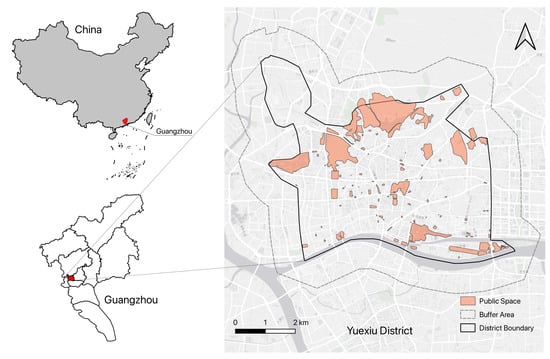
Figure 1. The location of the study area and public spaces.

3.2. Data Collection

This study employs a multi-source data integration approach to obtain spatiotemporal characteristic data of urban public spaces, primarily comprising Baidu Heat Map (BHM), Points of Interest (POI), building Area of Interest (AOI), and road network data. The BHM data are derived from Baidu Maps’ location-based services (LBS), representing aggregated and anonymized mobile phone positioning data that visualize population density distributions. These data serve as the fundamental dataset to calculate the vitality of public spaces across day and night periods. Previous studies have demonstrated that the Baidu heat map data provide a reliable representation of spatiotemporal crowd activity patterns and have been effectively validated for urban spatial analysis applications [13,41].

It is important to clarify the terminology used in this study. The term “heatmap” refers to a visualization technique that uses color gradients to represent data density or intensity, not actual temperature measurements. Throughout this paper, terms such as “heat values” are metaphorical expressions derived from the heatmap visualization method, representing population activity intensity rather than thermal comfort or temperature conditions. When discussing actual temperature-related factors (such as thermal comfort mentioned in the literature review), we explicitly use terms like “temperature” or “thermal comfort” to distinguish them from the metaphorical usage of “heat” in the context of population density visualization. For data characterizing urban public space environmental factors, POI data and road network data are sourced from OpenStreetMap, while building AOI vector data are obtained from Tencent Maps’ first quarter 2024 dataset. To ensure data precision, all spatial data were verified and calibrated using high-resolution satellite imagery from 2024, supplemented by field survey data to validate functional attributes and usage patterns of public spaces, thus ensuring the reliability of research data.

Data collection was conducted on 15 October 2024 (Thursday) and 19 October 2024 (Saturday). The selection criteria for these dates were (1) suitable temperature conditions with similar weather patterns on both days, (2) absence of pandemic control measures or lockdown restrictions, and (3) non-holiday periods that could represent typical daily activities of Guangzhou residents over one weekday and one weekend day. Data sampling was performed hourly from 8:00 AM to 2:00 AM the following day, producing 17 data samples per day. The temporal periods were classified as daytime (8:00 AM to 6:00 PM) and night-time (6:00 PM to 2:00 AM the following day). The collected data were spatially visualized on the QGIS 3.40 (QGIS Development Team, 2024), and data points outside the defined study area were filtered to ensure spatial consistency with the scope of the investigation.

3.3. Methods

This section elaborates on the research methodology employed in this study. The overall research logic and analytical framework are first introduced to guide the investigation. The measurement procedures for quantifying public space vitality across different temporal scenarios are then described, followed by the selection and operationalization of built environment factors that potentially influence vitality. Finally, the geographically weighted random forest model is presented as the analytical method to examine the spatiotemporal heterogeneity of these influences.

3.3.1. Research Framework

Figure 2 illustrates the research framework, which integrates data acquisition, indicator construction, spatiotemporal pattern analysis, and GWRF modeling.

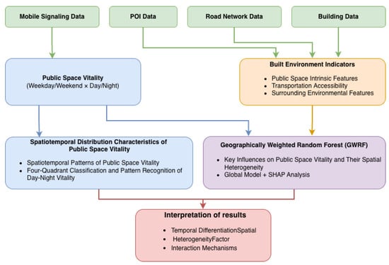
Figure 2. Research framework.

First, four types of spatial data sources are integrated: Baidu Heat Map (BHM), POI, road network, and building. The BHM data serve as the basis for quantifying public-space vitality across different temporal dimensions (weekday/weekend and daytime/night-time), whereas POI, road network, and building data are processed and categorized to construct an indicator system of factors influencing urban public-space vitality (see Table 1 for details).

Table 1. Urban public space vitality impact factors indicator system.

Dimension	Variable	Calculation Method	Data Source
Public Space Intrinsic Features	Area	Public space unit area calculated using $A=\sum (\mathrm{pixel}\mathrm{area}\times \mathrm{spatial}{\mathrm{resolution}}^2)$	Remote sensing imagery
Transportation Accessibility	Road intersection density	$D_{\mathrm{intersection}}={\displaystyle \frac{N_{\mathrm{intersections}}}{A_{\mathrm{service}}}}$	OpenStreetMap
	Public transport stops density	$D_{\mathrm{transit}}={\displaystyle \frac{N_{\mathrm{stops}}}{A_{\mathrm{service}}}}$	OpenStreetMap
	Local integration	$I_{\mathrm{local}}={\displaystyle \frac{1}{n}}{\sum }_{i=1}^n{\displaystyle \frac{1}{d_i}}$	DepthMap
Surrounding Environmental Features	Total building density	$D_{\mathrm{total}}={\displaystyle \frac{A_{\mathrm{all}\_\mathrm{buildings}}}{A_{\mathrm{buffer}}}}$ (1000 m buffer radius)	Tencent Map
	Residential density	$D_{\mathrm{res}}={\displaystyle \frac{A_{\mathrm{res}\_\mathrm{buildings}}}{A_{\mathrm{buffer}}}}$ (1000 m buffer radius)	Tencent Map
	Residential proportion	$R_{\mathrm{res}}={\displaystyle \frac{N_{\mathrm{res}\_\mathrm{buildings}}}{N_{\mathrm{total}\_\mathrm{buildings}}}}$ (1000 m buffer radius)	Tencent Map
	POI density	$D_{\mathrm{POI}}={\displaystyle \frac{N_{\mathrm{POI}}}{A_{\mathrm{service}}}}$	OpenStreetMap
	Traffic density	$D_{\mathrm{traffic}}={\displaystyle \frac{L_{\mathrm{road}}}{A_{\mathrm{service}}}}$	OpenStreetMap
	Public service density	$D_{\mathrm{services}}={\displaystyle \frac{N_{\mathrm{services}}}{A_{\mathrm{service}}}}$	OpenStreetMap

A = Area; N = Number of facilities/points; D = Density; $A_{\mathrm{service}}$ = Service area; $p_i$ = Proportion of category i; H = Shannon diversity index; $I_{\mathrm{transport}}$ = Transport integration index.

The study adopts a dual-track analytical approach. The spatiotemporal track focuses on the distribution patterns of public-space vitality, including the identification of spatiotemporal patterns and the application of a four-quadrant classification method to recognize day–night vitality regimes. Concurrently, the GWRF model is employed to analyze the relationship between built-environment indicators and public-space vitality, thereby identifying key influencing factors and their spatial heterogeneity under different temporal contexts. By synthesizing findings from both tracks, the framework elucidates the temporal differentiation and spatial heterogeneity of public-space vitality.

3.3.2. Public Space Day–Night Vitality Measurement

The urban vitality values of this study are based on Baidu heatmap data, using the kernel density estimate (KDE) method to quantify spatial activity. The study area is divided into regular 30 × 30-m grids, and the vitality value for each grid cell is calculated using the following formula:

$$f\left(x\right)={\displaystyle \frac{1}{nh}}\sum _{i=1}^{n}K\left({\displaystyle \frac{x-x_i}{h}}\right)$$

(1)

where $f\left(x\right)$ is the density estimate at location x, n is the total number of data points, h is the bandwidth parameter, K is the Gaussian kernel function, and $x_i$ is the location of the i-th data point. Vitality values reflect the frequency of population activities and the intensity of spatial usage within grid areas, providing comparable quantitative standards for spatial activity across different regions and periods. These values are dimensionless relative indices rather than absolute counts of individuals or devices, representing the aggregated intensity of human activities derived from mobile phone location-based services.

This study employs multi-source data fusion and spatial interpolation methods to process public space vitality data. First, the geographical information of 149 public spaces in the Yuexiu District was obtained from OpenStreetMap, with geometric centroids extracted and transformed to the UTM coordinate system (EPSG:32649) to ensure distance calculation accuracy. Second, the heatmap statistical data were loaded and aggregated by public space names to calculate average vitality values for daytime (8:00–18:00) and night-time (18:00–2:00) periods. Geographic and vitality data were merged through standardized name matching, with missing data estimated using the Inverse Distance Weighting (IDW) interpolation method, setting a search radius of 5 km, a maximum of 10 neighbors, and a power parameter of two. Finally, day–night vitality ratios were calculated to form a comprehensive dataset containing original data identifiers. This methodology effectively addresses data gaps, improves spatial coverage, and provides a reliable data foundation for subsequent public space vitality analysis.

3.3.3. Selection of Vitality Influencing Factors

Based on a review of the literature [7,13,17], the environmental characteristics influencing public space vitality can be categorized into three dimensions: intrinsic characteristics of the parcel, surrounding environmental characteristics, and transportation network attributes. Considering indicator applicability and data availability, this study selects 10 factors across these three dimensions to establish an indicator system for analyzing urban public space vitality (Table 1).

3.3.4. Geographically Weighted Random Forests

Geographically weighted random forest (GWRF) is an analytical method that integrates geographically weighted regression (GWR) with random forest (RF). This approach introduces a geographical weight matrix to dynamically adjust the contribution of neighboring spatial units during the decision tree construction process in random forest, effectively addressing the limitations of traditional global models that ignore spatial heterogeneity. Leveraging the ensemble learning mechanism of random forest, it automatically identifies complex nonlinear interactions among variables through collaborative exploration of high-dimensional feature space by multiple decision trees, quantifying the influence of different factors on vitality. This study employs the GWRF model to analyze the correlation between urban environmental characteristics and urban public space vitality, interpreting spatial heterogeneity in the data and determining how the importance of different variables varies across geographical space.

This study constructs a comprehensive indicator system comprising 10 independent variables: diversity score, local integration, total building density, residential density, residential proportion, POI density, traffic density, intersection density, public service density, and public space area. Using daytime and night-time vitality values as dependent variables, separate GWRF models were established for comparative diurnal analysis. The model employs a Gaussian kernel function to calculate spatial weights $w_{ij}=exp(-0.5\times {(d_{ij}/h)}^2)$, where bandwidth h is set as the median of all pairwise distances. For each target location, local random forest models are trained based on spatial weights ($n\_estimators=100$), extracting feature importance and calculating local $R^2$ values, ultimately obtaining global $R^2$ and RMSE to evaluate model performance. Through comparison of feature importance, local $R^2$ distribution, and prediction accuracy between daytime and night-time models, key factors influencing park vitality and their spatiotemporal variation characteristics are identified, with correlation analysis employed to validate the rationality of inter-variable relationships.

4. Results

4.1. Spatiotemporal Distribution Characteristics of Public Space Vitality

This subsection comprises two components: Section 4.1.1 presents the spatial distribution and statistical characteristics of vitality values across four temporal scenarios (weekday/weekend × daytime/night-time), revealing the overall spatiotemporal patterns. Section 4.1.2 applies a four-quadrant classification method to categorize public spaces based on their day–night vitality relationships, thereby identifying distinct temporal response patterns and examining how these patterns vary across different public space types.

4.1.1. Spatiotemporal Patterns of Public Space Vitality

Considering that the vitality of public spaces is not only reflected within their boundaries but also manifested through pedestrian activities in surrounding areas, which indicate the attractiveness and radiating effects of these spaces, this study establishes a 200-m buffer zone around each public space as the statistical unit. This distance corresponds to a walkable range (approximately 2–3 min walking time) and can encompass a sufficient number of $30\times 30$ m heat map grid cells, ensuring the stability and representativeness of the statistical results.

For the 200 m buffer zone of each public space, all heat values from the $30\times 30$ m grid points falling within the buffer area are extracted to form a heat value set $\{v_1,v_2,\dots ,v_N\}$, where $v_i$ represents the heat value of the i-th grid point, and N denotes the total number of grid points within the buffer zone. Three statistical indicators are calculated:

$$\mathrm{mean}={\displaystyle \frac{1}{N}}\sum _{i=1}^N{v}_i.$$

(2)

The mean heat value (Equation (1)) eliminates the impact of area differences among public spaces, facilitating cross-comparisons between public spaces of different scales. The sum of heat values (${\sum }_{i=1}^N{v}_i$) comprehensively considers both vitality intensity and spatial extent, better reflecting the attractiveness of public spaces. The count of heat points (N) indicates the data coverage within each buffer zone.

The mean heat values of public spaces in the Yuexiu District during daytime and night-time periods, calculated from the Baidu heat map data, were imported into QGIS for visualization and analysis (Figure 3). The map illustrates the spatial distribution patterns of public space vitality across four spatiotemporal scenarios: weekday vs. weekend, and daytime vs. night-time within the Yuexiu District. The visualization clearly reveals significant spatiotemporal heterogeneity in public space vitality. To facilitate visual comparison across different temporal scenarios, a unified color scale is applied to all four maps, with specific vitality value ranges for each period described in the text.

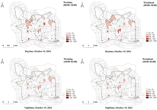
Figure 3. Spatiotemporal vitality patterns in the Yuexiu District’s public spaces: day-night and weekday-weekend variability.

In general, the levels of vitality of the public space on weekend are higher than on weekday. The mean heat value of daytime vitality on weekend is 47.51, exceeding the weekday value of 40.33; the mean night-time value is 33.10, surpassing the weekday value of 26.49. These values represent dimensionless indices reflecting relative population activity density. From a day–night perspective, daytime vitality (mean: 40.33–47.51) is generally higher than night-time vitality (mean: 26.49–33.10), though the spatial distribution patterns differ significantly. During daytime hours (8:00–18:00), vitality values range from 2 to 194. During night-time hours (18:00–02:00), the overall vitality level decreases (range: 2.7–128), though the spatial distribution pattern shows notable differences compared to daytime.

4.1.2. Four-Quadrant Classification and Pattern Recognition of Day–Night Vitality

This study conducts a day–night vitality pattern analysis of 149 public spaces in the Yuexiu District, employing a four-quadrant classification method [22] to categorize public spaces into four types based on the relationship between daytime and night-time vitality values and their respective medians: High Day–High Night (HD–HN), High Day–Low Night (HD–LN), Low Day–High Night (LD–HN), and Low Day–Low Night (LD–LN). During the data preprocessing stage, the Inverse Distance Weighting (IDW) interpolation method is applied to spatially complete the missing vitality values. Among the 149 public spaces, only three (2.0%) required IDW interpolation due to the absence of overlapping heatmap grid cells, while the remaining 146 (98.0%) obtained direct measurements from heatmap data. The IDW parameters (power = 2, max neighbors = 10, max distance = 5000 m) ensured spatial accuracy, with interpolated values falling within reasonable ranges consistent with the surrounding areas. This method fully considers the spatial distribution characteristics of heat values and significantly improves computational accuracy compared to simple statistical imputation methods. Through a multi-level missing value processing mechanism, all public spaces are ensured to be accurately classified. Based on this classification framework, this study conducts a systematic comparative analysis of vitality pattern distribution characteristics between weekday (15 October 2024) and weekend (19 October 2024). The classification results are spatially visualized using QGIS software, with different colors representing the spatial distribution patterns of the four vitality types across the Yuexiu District (Figure 4).

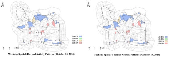
Figure 4. Four-quadrant classification of day–night vitality patterns in the Yuexiu District public spaces.

Spatial distributions reveal distinct patterns. LD–LN spaces predominantly concentrate in the northern and eastern peripheral areas of the Yuexiu District, indicating consistently low vitality throughout both day and night. HD–HN spaces scatter across central and southern districts, representing areas with sustained high activity levels. LD–HN and HD–LN spaces show limited distribution, suggesting that most public spaces do not experience dramatic day–night vitality transitions.

Public spaces in the Yuexiu District were extracted from OpenStreetMap (OSM) data and classified into six categories based on their functional attributes. A total of 149 public spaces were identified, distributed as follows: green spaces (n = 66, 44.3%), parks (n = 62, 41.6%), plazas (n = 7, 4.7%), fitness and sports facilities (n = 7, 4.7%), playgrounds (n = 3, 2.0%), and leisure venues (n = 3, 2.0%) (Figure 5a). Among these, green spaces and parks constitute the predominant public space types, accounting for 85.9% of the total distribution.

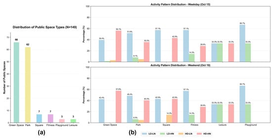
Figure 5. Analysis of day–night vitality patterns across public space types: (a) proportion of four-quadrant classifications by public space type and (b) comparison of four-quadrant classification across different types of public spaces: weekday vs. weekend.

The comparative analysis between weekday and weekend reveals variations in the temporal stability of vitality patterns across different types of public spaces (Figure 5b). Green spaces demonstrate high temporal stability (change rate of 6.1%, defined as the proportion of samples whose vitality patterns changed between weekday and weekend), with the HD–HN pattern predominating on both weekday and weekend (56.1% and 57.6%, respectively). However, the persistent polarization phenomenon (39.4% LD–LN on weekday, 42.4% on weekend) indicates significant spatial heterogeneity and accessibility differences within the green space system. Parks also show consistent pattern distributions between weekday and weekend (change rate of 11.3%), characterized by the coexistence of two dominant patterns: LD–LN (approximately 50%) and HD–HN (approximately 35–40%), reflecting functional differentiation across different periods and locations. In contrast, Fitness and Squares exhibit more pronounced pattern changes with the arrival of weekend (change rates of 28.6% and 14.3%, respectively), demonstrating sensitivity to leisure time shifts. Playgrounds and Leisure facilities (each n = 3, with limited sample sizes introducing certain specificity) are predominantly characterized by LD–LN and LD–HN patterns during both time periods, with change rates of 0%.

4.2. GWRF-Based Analysis of Built Environment Effects and Spatiotemporal Patterns

This subsection comprises four components that sequentially address model validation, variable relationships, factor importance, and spatial heterogeneity. Section 4.2.1 presents the GWRF model construction process and performance evaluation results. Section 4.2.2 examines the correlation patterns among variables and their temporal variations. Section 4.2.3 identifies key influencing factors and analyzes their importance across day–night and weekday–weekend scenarios. Section 4.2.4 reveals the spatial heterogeneity of built environment effects, examining how factor importance varies across different locations within the district.

4.2.1. GWRF Model Construction and Performance Evaluation

Model Construction Workflow. The GWRF model construction follows a standard spatial machine learning workflow comprising four key steps. First, standardization was applied to 10 feature variables across 149 public space samples using Z-score transformation to achieve a mean of zero and standard deviation of one. Second, a Gaussian kernel function was adopted to calculate the spatial weight matrix, formulated as follows:

$$w_i=exp\left(-0.5\times {\left({\displaystyle \frac{d_i}{h}}\right)}^2\right)$$

(3)

where $d_i$ represents the Euclidean distance between sample points and h denotes the bandwidth parameter. This function ensures that neighboring sample points receive higher weights, embodying the spatial correlation principle of Tobler’s First Law of Geography. Third, cross-validation was employed to determine the optimal spatial bandwidth of 2.76 km, balancing localized modeling precision with adequate sample size. Finally, a weighted random forest model was constructed for each spatial location with the following parameters: 100 trees, maximum depth of 10 layers, and minimum leaf node sample size of five.

Model Validation and Performance. To improve the model’s reliability and generalizability, commonly adopted validation practices in the geographically weighted modeling literature were followed [42,43]. Our validation approach comprises three components:

(1) goodness-of-fit metrics including global and local R², RMSE, and spatial stability assessment through Coefficient of Variation (CV) of local R² values; (2) spatial autocorrelation diagnostics using Moran’s I tests at both pre-modeling and post-modeling stages to confirm adequate capture of spatial dependencies; (3) residual analysis examining spatial distribution patterns and statistical properties to detect systematic bias.

The GWRF model demonstrated superior predictive performance across all temporal periods, with global R² values exceeding 0.88 (Table 2 and Table 3). Model performance varied systematically by time: weekday night-time models (R² = 0.9172) outperformed daytime models, while weekend models showed the reverse pattern. This reflects distinct spatial structures—night-time weekday vitality exhibits regular patterns linked to residential areas, whereas weekend daytime involves more complex, heterogeneous recreational and commercial activities, resulting in higher prediction errors.

Table 2. Daytime model performance comparison: weekday vs. weekend.

Evaluation Metrics	Weekday (Oct 15)	Weekend (Oct 19)	Difference	Change (%)
Model Performance
Global R2	0.9096 *	0.9060 *	−0.0036	−0.40%
RMSE	3.79	5.36	+1.57	+41.42%
Local R2 Minimum	0.8769	0.8717	−0.0052	−0.59%
Local R2 Mean	0.9014	0.8981	−0.0033	−0.37%
Local R2 Median	0.8967	0.8959	−0.0008	−0.09%
Local R2 Maximum	0.9336	0.9283	−0.0053	−0.57%
CV of Local R2 (%)	1.52	1.53	+0.01	+0.66%
Spatial Autocorrelation
Raw Vitality Moran’s I	0.1457 **	0.1681 **	+0.0224	+15.38%
Residual Moran’s I	−0.0315 (ns)	−0.0130 (ns)	—	—
Spatial Autocorrelation Reduction (%)	78.4	92.3	+13.9	—

* p < 0.001 for model significance; ** p < 0.05 for spatial autocorrelation; ns = not significant (p > 0.05). CV (Coefficient of Variation) measures the spatial stability of local R² values. CV < 2% indicates very high stability, and 2–3% indicates good stability. Spatial Autocorrelation Reduction = (Raw Moran’s I − |Residual Moran’s I|)/Raw Moran’s I × 100%, indicating the percentage of spatial clustering eliminated by the GWRF model.

Table 3. Night-time model performance comparison: weekday vs. weekend.

Evaluation Metrics	Weekday (Oct 15)	Weekend (Oct 19)	Difference	Change (%)
Model Performance
Global R2	0.9172 *	0.8880 *	−0.0292	−3.18%
RMSE	2.09	3.79	+1.70	+81.34%
Local R2 Minimum	0.8850	0.8357	−0.0493	−5.57%
Local R2 Mean	0.9119	0.8810	−0.0309	−3.39%
Local R2 Median	0.9093	0.8786	−0.0307	−3.38%
Local R2 Maximum	0.9395	0.9214	−0.0181	−1.93%
CV of Local R2 (%)	1.41	2.36	+0.95	+67.38%
Spatial Autocorrelation
Raw Vitality Moran’s I	0.1478 **	0.1444 **	−0.0034	−2.30%
Residual Moran’s I	−0.0248 (ns)	0.0159 (ns)	—	—
Spatial Autocorrelation Reduction (%)	83.2	89.0	+5.8	—

* p < 0.001 for model significance; ** p < 0.05 for spatial autocorrelation; ns = not significant (p > 0.05). CV (Coefficient of Variation) measures the spatial stability of local R² values. CV < 2% indicates very high stability, and 2–3% indicates good stability. Spatial Autocorrelation Reduction = (Raw Moran’s I − |Residual Moran’s I|)/Raw Moran’s I × 100%, indicating the percentage of spatial clustering eliminated by the GWRF model.

Temporal stability analysis revealed contrasting patterns. Daytime models maintained consistent performance across weekday and weekend (R² difference only 0.36%), while night-time models exhibited substantial variation (2.92 percentage points), with weekday performance considerably exceeding weekend. This confirms that daytime vitality follows stable spatial determinants regardless of day type, while night-time patterns are more temporally variable.

Diagnostic Analysis. Pre-modeling analysis revealed significant positive spatial autocorrelation in raw vitality data (Moran’s I = 0.1444–0.1681, all p < 0.05), justifying geographically weighted approaches. Post-modeling diagnostics demonstrated successful elimination of spatial autocorrelation, with all residual Moran’s I values becoming non-significant (p > 0.05) and near zero, representing 78.4–92.3% reduction compared to the original data (Figure 6). The reduction rate is calculated as: Reduction (%) = (|I_raw| − |I_residual|) / |I_raw| × 100%, where I_raw is the Moran’s I of original data and I_residual is the Moran’s I of model residuals.

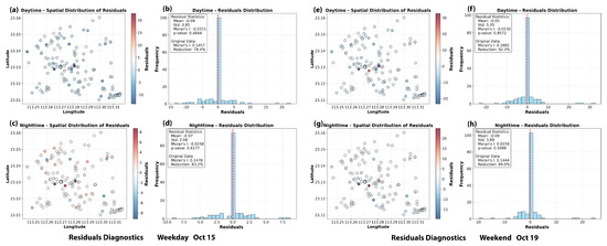
Figure 6. Spatial diagnostics of GWRF model residuals: (a–d) weekday models; (e–h) weekend models; (a,c,e,g) spatial distribution maps; and (b,d,f,h) residual histograms. Red dashed lines in residual histograms mark the zero baseline for reference.

Local R² distributions indicated consistent spatial stability (CV: 1.41–2.36%), with weekday models showing slightly tighter distributions than weekend models (Figure 7). Visual inspection of residuals revealed random spatial patterns without clustering, near-normal distributions centered at zero, and strong linear relationships in predicted vs. actual scatter plots (Figure 8). These diagnostics collectively confirm that GWRF achieves high predictive accuracy while satisfying fundamental spatial modeling assumptions, ensuring reliable interpretation of spatially varying relationships between urban form and vitality patterns.

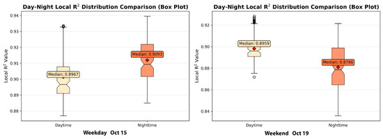
Figure 7. Box Plot Comparison of local R² distribution between daytime and night-time models.

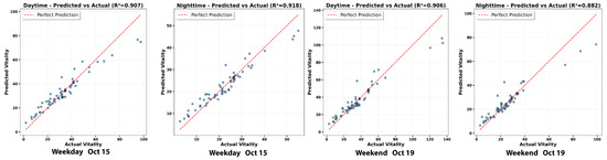
Figure 8. Predicted vs. actual vitality scatter plots across four temporal scenarios.

4.2.2. Temporal Variation Characteristics of Variable Correlations

The correlation analysis between variables revealed fundamental association patterns and the temporal heterogeneity characteristics of influencing factors (Figure 9). The results showed that correlations between various factors and vitality showed systematic differences in weekday–weekend and day–night cycles. Some variables showed strong correlations between them, while others showed relatively independent characteristics.

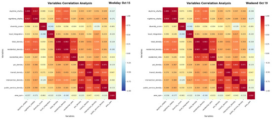
Figure 9. Correlation analysis of influencing factors.

Correlations between daytime and nightlife show weekday–weekend differences. Weekend periods showed a significantly higher correlation between day and night vitality (r = 0.959) compared to weekday (r = 0.917), indicating greater continuity and consistency in weekday vitality patterns. On the other hand, weekday showed a more pronounced diurnal differentiation, reflecting the structural influence of commuting patterns and functional zoning on day–night vitality dynamics.

The association between density variables and vitality showed temporal variations. During the week, the correlations of total building density with daytime vitality (r = 0.582) and night-time vitality (r = 0.621) were higher than weekend vitality (r = 0.546, night r = 0.563), indicating a greater dependence of weekday activities on the density of the urban built environment. The residential density showed similar patterns of association, with weekly daytime correlations (r = 0.623) exceeding weekend (r = 0.586). In particular, the correlation between the residence ratio and nightlife was higher during weekend (r = 0.287) than on weekday (r = 0.226), reflecting the greater dependence of weekend night activities on residential functions.

Some variables showed relatively independent characteristics. Diversity points generally show weak correlations with other variables (absolute values 0.24), indicating that functional mixtures, as a relatively independent dimension of urban forms, are not strongly constrained by density or other factors that influence vitality. The density of sections showed similar low correlations with most variables, representing the independent role of the network connectivity of the streets. Local integration, as a space syntax indicator, maintained moderate correlations with density variables (r = 0.20–0.42), reflecting the relative independence of the accessibility dimension. Public space areas showed weak negative correlations with vitality (r = −0.15 to −0.19), but weak correlations with other influencing factors, reflecting the particularity of the spatial scale factor.

4.2.3. Difference in Impact of Factors on Day–Night Vitality

The GWRF model revealed the differential importance of factors influencing public space vitality between daytime and night-time across different temporal contexts (Figure 10).

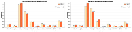
Figure 10. Feature importance comparison between daytime and night-time models: weekday vs. weekend.

On weekday (Oct 15), total density (total building density) emerged as the dominant factor for both periods, showing higher importance during night-time (41.3%) compared to daytime (38.2%). Residential density ranked second, with greater influence during daytime (27.0%) than night-time (23.0%). The residential ratio maintained similar importance across both periods (8.6% daytime vs. 8.7% night-time). Notably, the diversity score showed higher importance during night-time (5.0%) compared to daytime (3.4%), suggesting an enhanced role of functional diversity in night-time activities. Public space area demonstrated relatively high importance (10.4% daytime, 8.8% night-time), while other factors such as POI density, transit density, and public service density showed limited contributions (all below 6%). The greater daytime influence of residential density (27.0% vs. 23.0% night-time) suggests that daytime public space usage is more closely tied to local residential populations engaging in routine activities near their homes. In contrast, the higher night-time importance of total density (41.3% vs. 38.2% daytime) indicates that evening activities are less constrained by residential proximity and more attracted to areas with higher overall building density. This pattern is further supported by the increased night-time importance of POI density (1.6% vs. 1.1% daytime), suggesting that night-time activities show stronger associations with areas offering diverse amenities and services.

Weekend patterns (Oct 19) exhibited distinct shifts in factor importance. While total density remained the most critical factor, its daytime importance decreased to 35.6% (compared to 38.2% on weekday), though night-time importance remained stable at 40.9%. Residential density showed more pronounced day–night difference on weekend (32.2% daytime vs. 26.5% night-time), with enhanced daytime importance compared to weekday. Most notably, the residential ratio demonstrated substantially increased night-time importance (13.3%) compared to both weekend daytime (8.9%) and weekday levels (approximately 8.7%), indicating the heightened role of residential composition in weekend evening activities. Diversity score showed relatively low importance on weekend (2.5% daytime, 3.3% night-time), markedly lower than weekday levels. Public space area exhibited reduced weekend importance (8.5% daytime, 5.3% night-time) compared to weekday, while other factors, including POI, transit, intersection, and public service densities, maintained consistently low importance (all below 5%) across both temporal contexts. The enhanced daytime importance of residential density on weekend (32.2% vs. 27.0% on weekday) reflects increased leisure-time usage of public spaces by residential populations, with the small gap between total density (35.6%) and residential density (32.2%) indicating that weekend daytime activities are strongly tied to residential areas. The substantially elevated night-time importance of residential ratio (13.3%) suggests that weekend evening activities show stronger associations with residential community characteristics, indicating more neighborhood-oriented social gatherings compared to weekday patterns.

4.2.4. Spatial Heterogeneity of Built Environment Effects

Beyond the temporal differentiation of factor importance discussed above, the GWRF model reveals spatial heterogeneity in how built environment factors influence public space vitality across different locations within the district. Figure 11 and Figure 12 visualize the spatial distributions of local importance coefficients, with black dots representing public space locations. The coefficient of variation (CV) in Table 4 and Table 5 quantifies the degree of spatial heterogeneity for each factor.

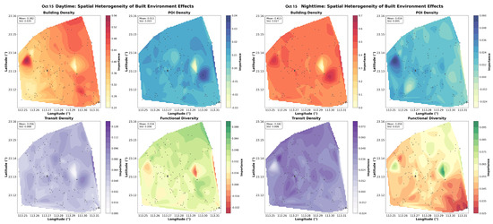
Figure 11. Spatial heterogeneity of built environment effects on weekday: local importance coefficients of four built environment factors.

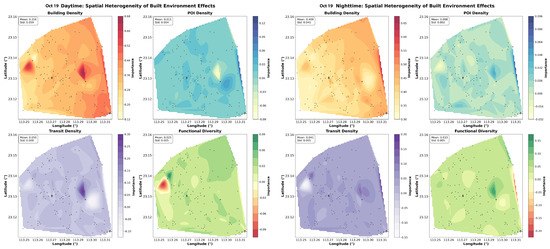
Figure 12. Spatial heterogeneity of built environment effects on weekend: local importance coefficients of four built environment factors.

Table 4. Spatial heterogeneity statistics of built environment factors on weekday.

Factor	Period	Mean	SD	Range	CV
Building Density	Day	0.383	0.035	0.278–0.482	0.092
	Night	0.413	0.027	0.356–0.462	0.065
POI Density	Day	0.011	0.003	0.006–0.017	0.231
	Night	0.016	0.005	0.008–0.029	0.278
Transit Density	Day	0.056	0.008	0.038–0.072	0.136
	Night	0.042	0.008	0.024–0.057	0.184
Functional Diversity	Day	0.034	0.007	0.019–0.058	0.189
	Night	0.050	0.010	0.027–0.068	0.198

CV = Coefficient of Variation, measuring the spatial variability of local importance values across different locations.

Table 5. Spatial heterogeneity statistics of built environment factors on weekend.

Factor	Period	Mean	SD	Range	CV
Building Density	Day	0.356	0.059	0.245–0.476	0.166
	Night	0.409	0.041	0.330–0.484	0.101
POI Density	Day	0.011	0.004	0.004–0.024	0.328
	Night	0.008	0.002	0.004–0.017	0.292
Transit Density	Day	0.050	0.008	0.028–0.069	0.154
	Night	0.041	0.005	0.030–0.055	0.129
Functional Diversity	Day	0.025	0.005	0.015–0.040	0.192
	Night	0.033	0.005	0.025–0.056	0.158

CV = Coefficient of Variation, measuring the spatial variability of local importance values across different locations.

As shown in Figure 11 and Table 4, weekday spatial heterogeneity exhibits distinct daytime and night-time patterns. During daytime, POI density exhibits the highest spatial variation (CV = 0.231). Building density shows moderate spatial heterogeneity (CV = 0.092) with importance coefficients averaging 0.382, while transit density (CV = 0.136) and functional diversity (CV = 0.189) display moderate heterogeneity. At night-time, building density effects increase in overall importance (mean: 0.413 vs. daytime 0.382) while becoming more spatially homogeneous (Std: 0.027 vs. daytime 0.055), with CV decreasing to 0.065. Meanwhile, POI density maintains high spatial variation (CV = 0.278), transit density shows CV = 0.184, and functional diversity exhibits CV = 0.198.

These day-to-night transitions reveal three key patterns. Building density effects become more homogeneous (CV decreases from 0.092 to 0.065). POI density heterogeneity intensifies (CV increases from 0.231 to 0.278), and spatial disparities in transit density and functional diversity widen (CV increases from 0.136 to 0.184 and from 0.189 to 0.198, respectively).

As shown in Figure 12 and Table 5, weekend spatial heterogeneity reveals intensified patterns. During daytime, POI density exhibits the most pronounced heterogeneity (CV = 0.328). Building density shows substantial spatial variation (CV = 0.166), while transit density (CV = 0.154) and functional diversity (CV = 0.192) also display clear spatial differentiation. At night-time, building density importance increases (mean: 0.409 vs. daytime 0.356), while spatial heterogeneity decreases (CV = 0.101). POI density exhibits CV = 0.292, transit density shows CV = 0.129, and functional diversity displays CV = 0.158.

The day-to-night transition reveals a convergence pattern: building density (CV decreasing from 0.166 to 0.101), POI density (CV decreasing from 0.328 to 0.292), transit density (CV decreasing from 0.154 to 0.129), and functional diversity (CV decreasing from 0.192 to 0.158) all exhibit reduced spatial variation.

The weekday–weekend comparison reveals contrasting spatial reorganization patterns. Weekdays show divergence, with night-time heterogeneity increasing for POI density, transit density, and functional diversity, indicating spatial concentration of activities. Weekends demonstrate convergence, with all factors exhibiting reduced spatial variation at night, suggesting more dispersed activity patterns. This contrast reflects the shift from routine-bound weekday behaviors anchored to residential-work commutes to more spatially flexible weekend recreational activities.

4.3. Factor Interaction Patterns

The above analysis elucidates the individual effects of built environment factors and their spatial heterogeneity; however, it has yet to address the following critical questions: how do these factors interact with each other? Do synergistic or competitive relationships exist among different factors, and how do these interaction patterns vary across temporal contexts?

To explore factor interactions, SHAP (SHapley Additive exPlanations) interaction analysis was applied to the global GWRF model to quantify how the effect of one built environment factor depends on the value of another [44]. SHAP interaction values measure synergistic effects (positive values, where combined effects exceed the sum of individual effects) vs. competitive or substitution effects (negative values, where one factor’s high value reduces another’s marginal benefit). Figure 13 and Figure 14 visualize the top factor interactions for weekday and weekend, respectively, revealing distinct temporal patterns in how built environment factors combine to influence public space vitality.

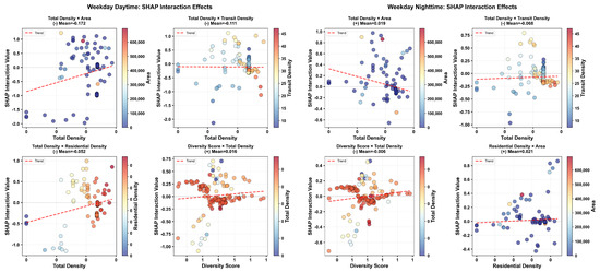
Figure 13. SHAP interaction effects on weekday: daytime (left) and night-time (right).

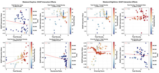
Figure 14. SHAP interaction effects on weekend: daytime (left) and night-time (right).

Weekday Interaction Patterns (Figure 13). On weekday daytime, the strongest interaction is total density × area (interaction strength: 0.489), exhibiting a competitive relationship (mean interaction value: −0.172). This negative interaction suggests that in high-density areas, a larger public space provides diminishing marginal benefits, while in low-density areas, a public space becomes more critical for vitality generation. Similarly, total density × transit density shows strong competitive interaction (0.325, −0.111), indicating spatial substitution, where high building density can partially compensate for lower transit accessibility in generating vitality. In contrast, diversity score × total density demonstrates synergistic interaction (0.213, 0.016), where functional diversity and building density reinforce each other—areas with both high density and diverse land uses achieve vitality levels exceeding the sum of individual effects. Residential density × residential ratio also shows synergistic effects (0.102, 0.010), suggesting that residential concentration works best when accompanied by high proportions of residential buildings. During weekday night-time, interaction patterns shift notably: total density × area transforms from competitive to synergistic (0.169, 0.019), indicating that larger public spaces in high-density areas become more valuable for evening activities. Total density × residential density also becomes synergistic (0.086, 0.047), reflecting the importance of residential support for night-time vitality in dense urban areas.

Weekend Interaction Patterns (Figure 14). Weekend daytime shows total density × area as the strongest interaction (0.618, 0.006), with moderate synergistic effects, indicating that public space area and building density work better together during leisure periods. However, total density × transit density remains competitive (0.328, −0.084), suggesting that weekend visitors rely less on transit density when building density is high, possibly due to automobile-based travel. Total density × residential density exhibits strong competitive interaction (0.348, −0.131), contrasting sharply with weekday night-time patterns. This suggests that on weekend, high building density areas dominated by commercial functions can attract visitors even without strong residential support. Diversity score × total density maintains moderate synergistic effects (0.279, 0.007), though weaker than on weekday. Local Integration × residential density shows strong synergistic interaction (0.116, 0.011), indicating that well-connected street networks enhance the vitality contribution of residential areas during weekend leisure activities. Weekend night-time demonstrates a return to density-centric patterns: total density × transit density remains competitive (0.262, −0.051), while diversity score × total density becomes strongly synergistic (0.233, 0.019), and total density × residential density shifts to synergistic (0.148, 0.098), mirroring weekday night-time patterns where residential support becomes critical.

Temporal Transitions in Factor Interactions. The total density × area interaction transitions from competitive (weekday daytime: −0.172) to synergistic (weekday night-time: 0.019, weekend daytime: 0.006), then back to competitive (weekend night-time: −0.027), demonstrating that the value of public space area in high-density areas varies with temporal activity patterns. Total density × residential density shows the most dramatic shift: strongly competitive on weekday daytime (−0.052) and weekend daytime (−0.131), but strongly synergistic during both night-time periods (weekday: 0.047, weekend: 0.098). This pattern reveals that residential density becomes a critical complement to building density, specifically during evening hours, when residents engage in proximate leisure activities. Diversity score × total density maintains consistently positive interactions across all periods, though with varying strength, confirming that functional diversity and building density form a stable synergistic relationship regardless of temporal context.

5. Discussion

The results presented in Section 4 reveal significant spatiotemporal heterogeneity in both public space vitality patterns and built environment effects. This section provides a mechanistic interpretation of these findings by examining two interconnected dimensions: the temporal differentiation mechanisms that drive day–night and weekday–weekend variations in factor importance, and the geographic variations in built environment factor effects across different locations and temporal scenarios. Together, these analyses elucidate the underlying processes through which temporal rhythms and spatial contexts interact to shape public space vitality.

5.1. Temporal Heterogeneous Effects of Built Environment on Vitality

The four-quadrant classification findings reveal distinct temporal mechanisms underlying built environment effects on public space vitality. Total building density, as the most critical factor, exhibits enhanced night-time importance across both weekday and weekend, consistent with existing studies [13,28,29]. This pattern reflects the spatiotemporal rhythm of urban population mobility. Daytime cross-regional commuting flows mean vitality depends on both local density and inter-regional mobility, while night-time reduced mobility confines activities to residential neighborhoods, making building density the dominant driver. Weekday–weekend comparison reveals attenuated effects on weekend, indicating reduced dependence on the immediate built environment when residents have greater temporal freedom.

Residential density exhibits opposite temporal patterns, showing greater daytime importance, particularly on weekend. This stems from two mechanisms: non-employed populations (elderly, children) constitute the main daytime users with limited mobility ranges, and high-density residential areas provide well-developed supporting facilities [45,46]. Specifically, elderly populations and children exhibit distinct spatiotemporal constraints that amplify residential density effects during daytime. In the Yuexiu District, the elderly population (aged 60+) accounts for 30.1% of the total population as of late 2024, ranking second among all districts in Guangzhou [47]. This substantial elderly demographic engages primarily in proximity-based activities due to reduced physical mobility and a preference for familiar environments. Research shows elderly residents prefer shady trees, peaceful settings, and accessible walking paths in neighborhood parks [48], with activity patterns concentrated in paved open spaces for social gatherings and pathways for walking exercises [49]. Their outdoor mobility is highly sensitive to environmental conditions, favoring cooler morning/evening hours and areas with greenery and pedestrian-friendly infrastructure [50]. Children’s activities are similarly constrained by parental supervision and school schedules, concentrating public space usage in neighborhood parks during after-school hours. High residential density areas provide larger user bases and support age-appropriate facilities that reinforce proximity-based usage. This demographic structure explains why residential density shows particularly strong daytime importance (27.0% on weekday, 32.2% on weekend), as these non-employed populations constitute the primary daytime users whose activity rarely extends beyond immediate residential neighborhoods. Beyond these daytime patterns, weekend intensification reflects the shift from workplace- to residence-centered activities. Residential proportion shows dramatic night-time enhancement on weekend, indicating that residential functions provide stable population bases for weekend nocturnal vitality.

Among accessibility factors, local integration and intersection density exhibit low overall importance but show notable temporal differentiation [41,46,51]. Local integration demonstrates contrasting weekday–weekend patterns. On weekday, daytime importance (2.3%) slightly exceeds night-time (1.7%), while weekend shows substantially elevated daytime importance (3.1%) compared to weekday. This weekend enhancement reflects greater freedom of movement as residents actively explore distant neighborhoods for leisure activities, with destination choices becoming more flexible and showing stronger preferences for areas with high transportation network connectivity [7]. During weekday daytime, most individuals remain in relatively fixed workplaces, rendering public space users primarily lunch-break crowds and non-working populations whose activity ranges prioritize proximity. Regardless of weekday or weekend, night-time importance remains relatively low (1.7% and 2.4%, respectively), as night-time activities are confined to spaces near residences within walking distance, reducing dependence on broader transportation networks.

Intersection density exhibits pronounced weekday–weekend contrasts. Weekdays show distinctive diurnal variation, with night-time importance (3.2%) more than doubling daytime importance (1.5%). This pattern may stem from proximate activity patterns, as individuals tend to select nearby leisure venues after work, where dense intersections offer more destination options within walking range. In contrast, weekend maintains temporal stability (1.7% daytime, 1.5% night-time) with consistently low importance. With more ample time for cross-regional travel on weekend, people rely more on macro-level transportation accessibility rather than micro-level road intersection density, underscoring the context-dependent role of intersection density in proximate vs. cross-regional mobility.

5.2. Geographic Variations in the Influence of Built Environment Factors

The four-quadrant classification identified LD–LN zones (consistently low vitality) concentrated in the northern periphery and southeastern corner. The spatial heterogeneity maps (Figure 11 and Figure 12) reveal different built environment patterns underlying this persistence. Northern LD–LN areas exhibit moderate building density importance but low importance for POI density, transit density, and functional diversity, indicating these areas have residential populations but lack commercial facilities, transit access, and functional mix necessary for vitality generation. Southeastern zones exhibit low importance across all four factors, suggesting both insufficient residential population and land uses incompatible with public space vitality.

Weekday–weekend comparisons reveal contrasting spatial patterns [20,52]. On weekday, night-time shows increased heterogeneity for POI, transit, and functional diversity, with importance concentrating in central areas while peripheral LD–LN zones remain low. Building density shows the opposite trend, becoming more spatially uniform at night. Weekends show reduced heterogeneity for all factors, with more uniform distributions. However, this spatial homogenization does not equalize vitality—LD–LN zones remain low because they possess lower absolute quantities of POIs, transit services, and functional diversity, regardless of how importance patterns distribute spatially.

These contrasting weekday–weekend patterns are fundamentally driven by socioeconomic and cultural factors. From a time-space perspective [53], these divergent patterns reflect how institutional, economic, and cultural forces shape distinct spatiotemporal regimes. On weekdays, institutional constraints—fixed schedules, centralized employment, and transit-dependent commuting—concentrate night-time activities around residential and commercial hubs, amplifying spatial heterogeneity [20,54]. Limited evening time and job-housing imbalance further reinforce this concentration by constraining mobility to proximity-based activities. In contrast, weekend free individuals from temporal-spatial rigidities, enabling leisure-oriented mobility toward diverse destinations—particularly natural hills and coastal areas. This expanded spatial accessibility, reinforced by cultural preferences for family-oriented outdoor recreation [46], results in more dispersed vitality patterns [53,54].

Beyond these temporal variations in spatial patterns, the GWRF model also reveals differential stability characteristics among built environment factors [55]. Building density maintains stable spatial patterns across temporal periods, while POI density and functional diversity vary spatially across different periods. This explains why some areas maintain stable vitality while others fluctuate temporally.

5.3. Factor Interaction Mechanisms

The SHAP interaction analysis reveals a fundamental characteristic of urban vitality generation. Built environment factors do not operate independently but interact through synergistic or competitive mechanisms that vary across temporal contexts [33]. These complex nonlinear interaction relationships and their significant temporal dependencies provide more refined and dynamic planning guidance for enhancing urban public space vitality. The following differentiated, temporally adaptive planning and design recommendations are proposed based on major interaction patterns:

Promoting “Density + Diversity” Mixed-Use Development. Diversity score and total density maintain stable positive synergistic interactions across all temporal periods. In urban renewal and redevelopment, priority should be given to mixed-use configurations (residential + commercial + cultural + recreational) to achieve multiplicative effects. This approach is particularly effective in areas with high vitality fluctuations, reducing disparities between different time periods.

Strengthening Residential Support for Night-time Vitality. Total density × residential density shifts from strong competition during daytime to strong synergy during both night-time periods, indicating that night-time activities are dominated by residents’ proximate leisure behavior, making residential density an indispensable complement to building density. Planning interventions should prioritize residential function enhancement in areas targeting night-time vitality improvement.

Context-Sensitive Public Space Area Planning. Total density × area exhibits a clear temporal cycle: competitive during weekday daytime, synergistic during weekday night-time and weekend daytime, then competitive again during weekend night-time. This demonstrates that the marginal benefit of large public spaces in high-density environments is highly dependent on activity types. High-density areas should not blindly pursue oversized plazas or green spaces; instead, priority should be given to improving space utilization efficiency and maximizing vitality capacity during leisure periods.

Transit-Density Substitution in Planning Strategies. The competitive interaction between total density and transit density during weekday daytime reveals substitution relationships. In high-density areas, building density can partially compensate for lower transit accessibility. However, in peripheral areas with high vitality fluctuations, addressing transit density deficiencies should be prioritized to enhance overall accessibility and vitality generation capacity.

6. Conclusions and Limitations

6.1. Conclusions

This study investigated the spatiotemporal heterogeneity of public space vitality and its built environment determinants across 149 public spaces in the Yuexiu District, Guangzhou, using the geographically weighted random forest model to examine four temporal scenarios.

This research demonstrates that public space vitality emerges from spatiotemporal coupling between built environment configurations and temporal activity patterns, rather than being a static spatial attribute. Methodologically, the GWRF model effectively captures spatial non-stationarity and nonlinear relationships, revealing localized mechanisms that conventional global models fail to detect.

The findings reveal significant spatiotemporal differentiation: Public space vitality varies substantially between day and night, weekday and weekend, while built environment impacts exhibit both temporal variation and spatial non-stationarity, with different factors dominating in different temporal contexts and spatial locations. The four-quadrant classification identified four distinct vitality patterns, with LD–LN spaces (consistently low vitality) concentrated in peripheral areas and HD–HN spaces (sustained high vitality) distributed across central districts. Weekday–weekend comparison reveals contrasting spatial reorganization patterns. Weekdays show divergence with night-time heterogeneity increasing for POI density, transit density, and functional diversity, while weekend demonstrates convergence with all factors exhibiting reduced spatial variation at night, reflecting the shift from routine-bound weekday behavior to spatially flexible weekend recreational activities.

These spatiotemporal patterns have direct implications for urban planning practice. First, recognizing diurnal differentiation patterns, planning interventions should provide temporally appropriate facility configurations: prioritizing night-time service facilities and lighting in high-density residential areas while supporting daytime activities for non-working populations. Second, addressing weekday–weekend differences requires multi-scale accessibility improvements: enhancing regional transportation connectivity for weekend leisure travel while refining community-scale pedestrian networks for weekday evening activities. Third, spatial heterogeneity analysis identifies priority intervention zones where high building density coexists with low functional mix. In these areas, supplementing diverse commercial and public service facilities is recommended to optimize community life circle configurations and enhance residents’ daily convenience.

Furthermore, the SHAP interaction analysis reveals that built environment factors do not operate independently but interact through synergistic or competitive mechanisms that vary across temporal contexts. Diversity score and total density maintain stable synergistic interactions across all periods, while total density and residential density exhibit dramatic temporal transitions from competitive during daytime to synergistic during night-time, demonstrating that the same socioeconomic forces driving temporal activity patterns also shape factor interaction mechanisms at different periods. This finding necessitates a shift from factor-by-factor optimization to interaction-aware planning strategies that maximize synergistic effects while minimizing competitive trade-offs across different temporal scenarios.

6.2. Limitations

The Baidu location-based services (LBS) data serve as a reliable proxy for human activity and interaction by capturing the dynamic distribution of the population across urban space; however, they cannot fully represent all age and social groups—particularly the elderly—or encompass all types of activity.

This study focuses primarily on quantifiable attributes of the built-environment that shape the diurnal characteristics of the vitality of public spaces, thereby overlooking the critical roles of qualitative factors such as aesthetic quality, perceived safety, and social atmosphere. These elements also exert substantial influence on vitality, which warrants deeper exploration in future research.

The temporal scope of this study is limited to data collected from only two dates (one weekday and one weekend in October 2024), which constrains the representation of seasonal variations in public space vitality. Different seasons may exhibit distinct activity patterns due to variations in weather conditions, daylight hours, and seasonal events, which are not captured in this analysis.

The findings were based of a single case study in Guangzhou’s Yuexiu District, and their generalizability to cities with differing morphological, cultural, and socioeconomic profiles remains to be validated. Future investigations could enhance theoretical and methodological transferability through multi-source data fusion, cross-seasonal comparisons, and multi-city validation.

References

- Huang, B.; Zhou, Y.; Li, Z.; Song, Y.; Cai, J.; Tu, W. Evaluating and characterizing urban vibrancy using spatial big data: Shanghai as a case study. Environ. Plan. B Urban Anal. City Sci. 2020, 47, 1543–1559. [Google Scholar] [CrossRef]
- Wu, C.; Ye, X.; Ren, F.; Du, Q. Check-in behaviour and spatio-temporal vibrancy: An exploratory analysis in Shenzhen, China. Cities 2018, 77, 104–116. [Google Scholar] [CrossRef]
- Lopes, M.N.; Camanho, A.S. Public Green Space Use and Consequences on Urban Vitality: An Assessment of European Cities. Soc. Indic. Res. 2013, 113, 751–767. [Google Scholar] [CrossRef]
- Jacobs, J. The Death and Life of Great American Cities; Random House: New York, NY, USA, 1961. [Google Scholar]
- Gehl, J. Life Between Buildings: Using Public Space; Van Nostrand Reinhold: New York, NY, USA, 1987. [Google Scholar]
- Montgomery, J. Making a City: Urbanity, Vitality and Urban Design. J. Urban Des. 1998, 3, 93–116. [Google Scholar] [CrossRef]
- Li, X.; Li, Y.; Jia, T.; Zhou, L.; Hijazi, I.H. The Six Dimensions of Built Environment on Urban Vitality: Fusion Evidence from Multi-Source Data. Cities 2022, 121, 103482. [Google Scholar] [CrossRef]
- Ta, N.; Zeng, Y.; Zhu, Q.; Wu, J. Understanding community rhythm from a spatiotemporal behavior perspective. Hum. Geogr. 2023, 38, 34–43. [Google Scholar] [CrossRef]
- Silm, S.; Ahas, R. Ethnic Differences in Activity Spaces: A Study of Out-of-Home Nonemployment Activities with Mobile Phone Data. Ann. Assoc. Am. Geogr. 2014, 104, 542–559. [Google Scholar] [CrossRef]
- Niu, H.; Silva, E.A. Crowdsourced Data Mining for Urban Activity: Review of Data Sources, Applications, and Methods. J. Urban Plan. Dev. 2020, 146, 04020007. [Google Scholar] [CrossRef]
- Li, X.; Kozlowski, M.; Salih, S.A.; Ismail, S.B. Evaluating the Vitality of Urban Public Spaces: Perspectives on Crowd Activity and Built Environment. Archnet-IJAR Int. J. Archit. Res. 2025, 19, 562–583. [Google Scholar] [CrossRef]
- Qin, L.; Zong, W.; Peng, K.; Zhang, R. Assessing Spatial Heterogeneity in Urban Park Vitality for a Sustainable Built Environment: A Case Study of Changsha. Land 2024, 13, 480. [Google Scholar] [CrossRef]
- Fan, Z.; Duan, J.; Luo, M.; Zhan, H.; Liu, M.; Peng, W. How Did Built Environment Affect Urban Vitality in Urban Waterfronts? A Case Study in Nanjing Reach of Yangtze River. ISPRS Int. J. Geo-Inf. 2021, 10, 611. [Google Scholar] [CrossRef]
- Xia, C.; Yeh, A.G.O.; Zhang, A. Analyzing spatial relationships between urban land use intensity and urban vitality at street block level: A case study of five Chinese megacities. Landsc. Urban Plan. 2020, 193, 103669. [Google Scholar] [CrossRef]
- Zeng, C.; Song, Y.; He, Q.; Shen, F. Spatially explicit assessment on urban vitality: Case studies in Chicago and Wuhan. Sustain. Cities Soc. 2018, 40, 296–306. [Google Scholar] [CrossRef]
- Zheng, Y.; Ye, R.; Hong, X.; Tao, Y.; Li, Z. What Factors Revitalize the Street Vitality of Old Cities? A Case Study in Nanjing, China. ISPRS Int. J. Geo-Inf. 2024, 13, 282. [Google Scholar] [CrossRef]
- Yu, B.; Sun, J.; Wang, Z.; Jin, S. Influencing Factors of Street Vitality in Historic Districts Based on Multisource Data: Evidence from China. ISPRS Int. J. Geo-Inf. 2024, 13, 277. [Google Scholar] [CrossRef]
- Liang, S.; Lu, M. Computer vision framework for site-scale multidimensional vitality assessment: Lakeside waterfront spaces as a testing ground. Habitat Int. 2025, 166, 103603. [Google Scholar] [CrossRef]
- Zhang, J.; Li, X.; Lian, H.; Li, H.; Zhang, J. Day–Night Synergy between Built Environment and Thermal Comfort and Its Impact on Pedestrian Street Vitality: Beijing–Chengdu Comparison. Buildings 2025, 15, 2118. [Google Scholar] [CrossRef]
- Chen, Y.; Yu, B.; Shu, B.; Yang, L.; Wang, R. Exploring the Spatiotemporal Patterns and Correlates of Urban Vitality: Temporal and Spatial Heterogeneity. Sustain. Cities Soc. 2023, 91, 104440. [Google Scholar] [CrossRef]
- Liu, S.; Zhu, Z.; Gao, Y.; Wang, S.; Zhou, Y. Exploring Factors behind Weekday and Weekend Variations in Public Space Vitality in Traditional Villages, Using Wi-Fi Sensing Method. ISPRS Int. J. Geo-Inf. 2025, 14, 386. [Google Scholar] [CrossRef]
- Zhuo, B.; Wang, Z.; Chen, T.; Tian, Z. Urban Vitality Characters at Day and Night in Qingdao. Planners 2021, 37, 94–100. [Google Scholar]
- Xu, X.; Xu, X.; Guan, P.; Ren, Y.; Wang, W.; Xu, N. The Cause and Evolution of Urban Street Vitality under the Time Dimension: Nine Cases of Streets in Nanjing City, China. Sustainability 2018, 10, 2797. [Google Scholar] [CrossRef]
- Wang, Y.; Dewancker, B.J.; Qi, Q. Citizens’ preferences and attitudes towards urban waterfront spaces: A case study of Qiantang riverside development. Environ. Sci. Pollut. Res. 2020, 27, 45787–45801. [Google Scholar] [CrossRef]
- Xu, G.; Su, J.; Xia, C.; Li, X.; Xiao, R. Spatial mismatches between nighttime light intensity and building morphology in Shanghai, China. Sustain. Cities Soc. 2022, 81, 103851. [Google Scholar] [CrossRef]
- Yue, Y.; Zhuang, Y.; Yeh, A.G.O.; Xie, J.Y.; Ma, C.L.; Li, Q.Q. Measurements of POI-based mixed use and their relationships with neighbourhood vibrancy. Int. J. Geogr. Inf. Sci. 2017, 31, 658–675. [Google Scholar] [CrossRef]
- Guo, Z.; Luo, K.; Yan, Z.; Hu, A.; Wang, C.; Mao, Y.; Niu, S. Assessment of the street space quality in the metro station areas at different spatial scales and its impact on the urban vitality. Front. Archit. Res. 2024, 13, 1270–1287. [Google Scholar] [CrossRef]
- Ye, Y.; Li, D.; Liu, X. How block density and typology affect urban vitality: An exploratory analysis in Shenzhen, China. Urban Geogr. 2018, 39, 631–652. [Google Scholar] [CrossRef]
- Mouratidis, K.; Poortinga, W. Built environment, urban vitality and social cohesion: Do vibrant neighborhoods foster strong communities? Landsc. Urban Plan. 2020, 204, 103951. [Google Scholar] [CrossRef]
- Tu, W.; Zhu, T.; Xia, J.; Zhou, Y.; Lai, Y.; Jiang, J.; Li, Q. Portraying the spatial dynamics of urban vibrancy using multisource urban big data. Comput. Environ. Urban Syst. 2020, 80, 101428. [Google Scholar] [CrossRef]
- Zhang, A.; Li, W.; Wu, J.; Lin, J.; Chu, J.; Xia, C. How can the urban landscape affect urban vitality at the street block level? A case study of 15 metropolises in China. Environ. Plan. B Urban Anal. City Sci. 2021, 48, 1245–1262. [Google Scholar] [CrossRef]
- Zhang, J.; Liu, X.; Tan, X.; Jia, T.; Senousi, A.M.; Huang, J.; Yin, L.; Zhang, F. Nighttime Vitality and Its Relationship to Urban Diversity: An Exploratory Analysis in Shenzhen, China. IEEE J. Sel. Top. Appl. Earth Obs. Remote Sens. 2021, 15, 309–322. [Google Scholar] [CrossRef]
- Xu, Y.; Mao, W.; Hu, S. Unveiling the Pulse of Urban Metro Stations: A TOD-driven Approach to Measuring Vibrancy Using Geographically Weighted Random Forest. Int. J. Digit. Earth 2025, 18, 2524054. [Google Scholar] [CrossRef]
- Li, H.; He, L. Park Development, Potential Measurement, and Site Selection Study Based on Interpretable Machine Learning—a Case Study of Shenzhen City, China. ISPRS Int. J. Geo-Inf. 2025, 14, 184. [Google Scholar] [CrossRef]
- Guangzhou Municipal Bureau of Statistics and National Bureau of Statistics Guangzhou Survey Team. Guangzhou Statistical Bulletin on National Economic and Social Development 2021; Statistical Bulletin, Guangzhou Municipal Bureau of Statistics: Guangzhou, China, 2022. (In Chinese)
- Liu, Y.; Zhang, Y.; Zhang, X.; Han, F.; Zhao, Y. A Geographical Perspective on the Formation of Urban Nightlife Landscape. Humanit. Soc. Sci. Commun. 2023, 10, 483. [Google Scholar] [CrossRef]
- Ren, W.; Lu, P.; Wang, Y.; Hong, X.C. Understanding the Association between Urban Noise and Nighttime Light in China. Sci. Rep. 2024, 14, 31472. [Google Scholar] [CrossRef]
- Guangzhou Municipal Bureau of Statistics. Guangzhou Population Census Yearbook-2020; Guangzhou Municipal Bureau of Statistics: Guangzhou, China, 2022.
- Guangzhou Yuexiu District People’s Government. Notice on the Issuance of Yuexiu District Territorial Spatial Master Plan (2021–2035); Government Document No. Yuefu [2025], 9, 2025; Guangzhou Yuexiu District People’s Government: Guangzhou, China, 2025. (In Chinese)
- Francis, J.; Giles-Corti, B.; Wood, L.; Knuiman, M. Creating Sense of Community: The Role of Public Space. J. Environ. Psychol. 2012, 32, 401–409. [Google Scholar] [CrossRef]
- Dong, Q.; Cai, J.; Chen, S.; He, P.; Chen, X. Spatiotemporal Analysis of Urban Green Spatial Vitality and the Corresponding Influencing Factors: A Case Study of Chengdu, China. Land 2022, 11, 1820. [Google Scholar] [CrossRef]
- Khan, S.N.; Li, D.; Maimaitijiang, M. A Geographically Weighted Random Forest Approach to Predict Corn Yield in the US Corn Belt. Remote Sens. 2022, 14, 2843. [Google Scholar] [CrossRef]
- Georganos, S.; Grippa, T.; Niang Gadiaga, A.; Linard, C.; Lennert, M.; Vanhuysse, S.; Mboga, N.; Wolff, E.; Kalogirou, S. Geographical Random Forests: A Spatial Extension of the Random Forest Algorithm to Address Spatial Heterogeneity in Remote Sensing and Population Modelling. Geocarto Int. 2021, 36, 121–136. [Google Scholar] [CrossRef]
- Gao, F.; Deng, X.; Liao, S.; Liu, Y.; Chen, W.; Li, G. Comparing Visitation Patterns in Distinct Types of Parks Using Geospatial Data and Interpretable Machine Learning. Urban For. Urban Green. 2025, 112, 128986. [Google Scholar] [CrossRef]
- Wang, F.; Zhao, M.X.; Meng, Q.L. Analysis of the vitality measurement and correlation factors of urban waterfront space. IOP Conf. Ser. Earth Environ. Sci. 2020, 612, 012013. [Google Scholar] [CrossRef]
- Zhu, J.; Lu, H.; Zheng, T.; Rong, Y.; Wang, C.; Zhang, W.; Yan, Y.; Tang, L. Vitality of urban parks and its influencing factors from the perspective of recreational service supply, demand, and spatial links. Int. J. Environ. Res. Public Health 2020, 17, 1615. [Google Scholar] [CrossRef]
- Guangzhou Civil Affairs Bureau. Statistical Data on Elderly Population and Aging Affairs in Guangzhou City for 2024; Technical Report; Guangzhou Civil Affairs Bureau: 2025. Released on 20 May 2025. Official Announcement with Attached PDF Containing Detailed Statistics. Available online: http://mzj.gz.gov.cn/gk/zdlyxxgk/ylfwxx/content/post_10271932.html (accessed on 9 January 2026).
- Veitch, J.; Ball, K.; Rivera, E.; Loh, V.; Deforche, B.; Best, K.; Timperio, A. What Entices Older Adults to Parks? Identification of Park Features That Encourage Park Visitation, Physical Activity, and Social Interaction. Landsc. Urban Plan. 2022, 217, 104254. [Google Scholar] [CrossRef]
- Zhai, Y.; Li, D.; Wu, C.; Wu, H. Spatial Distribution, Activity Zone Preference, and Activity Intensity of Senior Park Users in a Metropolitan Area. Urban For. Urban Green. 2023, 79, 127761. [Google Scholar] [CrossRef]
- Močnik, Š.; Moogoor, A.; Yuen, B. Exploring Facilitators and Barriers of Older Adults’ Outdoor Mobility: A Walk-along Study in Singapore. J. Transp. Health 2022, 26, 101386. [Google Scholar] [CrossRef]
- Yang, Y.; Ma, Y.; Jiao, H. Exploring the Correlation between Block Vitality and Block Environment Based on Multisource Big Data: Taking Wuhan City as an Example. Land 2021, 10, 984. [Google Scholar] [CrossRef]
- Park, S.; Lee, D. Exploring the Spatiotemporal Heterogeneities in Urban Vitality Through Scalable Proxies from Mobile Data. Land 2024, 13, 1772. [Google Scholar] [CrossRef]
- Huang, Y.; Du, J.; Chen, M.; Lin, Y.; Huang, S.; Cai, Y. Evaluating the Spatial-Temporal Impact of Urban Nature on Urban Vitality in Vancouver: A Social Media and GPS Data Approach. Land Use Policy 2026, 160, 107824. [Google Scholar] [CrossRef]
- Li, Z.; Zhao, G. Revealing the Spatio-Temporal Heterogeneity of the Association between the Built Environment and Urban Vitality in Shenzhen. ISPRS Int. J. Geo-Inf. 2023, 12, 433. [Google Scholar] [CrossRef]
- Tang, S.; Ta, N. How the Built Environment Affects the Spatiotemporal Pattern of Urban Vitality: A Comparison among Different Urban Functional Areas. Comput. Urban Sci. 2022, 2, 39. [Google Scholar] [CrossRef] [PubMed]
Disclaimer/Publisher’s Note: The statements, opinions and data contained in all publications are solely those of the individual author(s) and contributor(s) and not of MDPI and/or the editor(s). MDPI and/or the editor(s) disclaim responsibility for any injury to people or property resulting from any ideas, methods, instructions or products referred to in the content. |
© 2026 by the authors. Licensee MDPI, Basel, Switzerland. This article is an open access article distributed under the terms and conditions of the Creative Commons Attribution (CC BY) license.