Abstract
Fly ash-based geopolymer concrete (FAGC) is a sustainable alternative to Portland cement concrete, offering significant reductions in carbon emissions while maintaining sufficient strength. This study proposes a three-stage framework for developing empirical formulae to accurately and interpretably predict FAGC compressive strength. In the first stage, predictive models were developed using linear regression (LR), deep neural network (DNN), and residual neural network (ResNet) approaches. Among these, the ResNet model achieved the highest predictive accuracy and effectively captured the complex nonlinear relationship between mix components, curing conditions, and compressive strength. In the second stage, global sensitivity analysis identified sodium silicate content, curing time, sodium hydroxide molarity, and water content as the most influential variables. Additionally, the interaction between fine aggregate content and curing temperature was found to have a substantial effect on strength development. In the final stage, an empirical formula was developed based on key variables and their interactions, providing a simple yet reliable tool for practical strength prediction with reduced computational requirements. The proposed framework is expected to bridge the gap between machine-learning prediction and applicability to support mix design optimisation and promote the wider adoption of sustainable geopolymer concrete in construction applications.
1. Introduction
1.1. Background
Fly ash-based geopolymer concrete (FAGC) is widely recognised as one of the most prominent and extensively studied types of sustainable concrete. The term “geopolymer” was first introduced and patented in 1978 by Joseph Davidovits [1], who proposed an alternative to ordinary Portland cement (OPC) by using aluminosilicate sources, derived from industrial by-products activated by alkaline activator. Davidovits’ motivation stemmed from growing awareness of the environmental burden posed by OPC, which is a major contributor to greenhouse gas emission. As of today, the cement industry is responsible for up to 5–8% of global CO2 emissions annually [2]. With an estimated emission factor of 0.58 tonnes of CO2 per tonne of cement produced [3], and a global cement production volume of approximately 4.1 billion tonnes [4], this translates to roughly 2.38 billion tonnes of CO2 emitted from cement manufacturing alone. These alarming figures have shown the urgent need to transition toward more sustainable cementitious materials. One such alternative is FAFC, which has demonstrated a significantly lower environmental impact compared to OPC concrete, with 37–63% reduction depending on the type of fly ash used, curing methods, and mix design parameters [5,6,7]. In addition to its environmental advantages, FAGC also offers economic benefits, achieving up to 30% cost reduction compared to OPC concrete, primarily due to the use of industrial by-product, fly ash, and the elimination of energy-intensive clinker production [5]. FAGC is primarily composed of low-calcium fly ash (commonly classified as Class F), which acts as the primary aluminosilicate source. Fly ash is a by-product generated from coal combustion in thermal power plants, consisting mainly silicon dioxide (SiO2) and aluminium oxide (Al2O3) [8]. The binder is formed through the activation of fly ash using a combination of alkaline activators, typically sodium hydroxide (NaOH) and sodium silicate solution (Na2SiO3). The result is a type of cement-free material that not only exhibits competitive compressive strength but also shows excellent performance in aggressive environment.
To date, a substantial number of studies have been dedicated to FAGC, with numerous studies examining its physical, mechanical, and durability properties. Among these, compressive strength remains the most widely investigated and critical material property, not only for geopolymer concrete but for all cementitious materials. FAGC has demonstrated the ability to achieve a compressive strength of up to 70 MPa [9,10,11]. FAGC’s compressive strength is influenced by a wide range of factors, including mix proportions [12,13], Na2SiO3/NaOH ratio, NaOH molarity [12,14], and curing time and temperature [11,15]. Luan et al. [12] reported a 39% increase in strength when NaOH concentration was raised from 11.5 mol/L to 15.5 mol/L, according to the microstructural evidence obtained from scanning electron microscope (SEM) and X-ray diffraction (XRD) tests. Similarly, curing conditions also play a vital role [15,16,17]. Rajput et al. [15] found that curing at 60 °C was optimal for achieving high strength, with temperatures above this threshold leading to a decline in performance. Verma et al. [17] observed that a shorter curing duration of 24 h resulted in higher compressive strength compared to longer durations (up to 72 h), suggesting that early strength gain in FAFC can be rapid under proper conditions. In addition to binder chemistry and curing, aggregates’ content and properties significantly affect FAGC strength [13,18]. Malkawi [13] found that increasing the proportion of coarse aggregates (from 55% to 85% of total aggregate volume) resulted in a strength reduction of approximately 50%. This was attributed to a reduction in the binding matrix available to form a continuous geopolymer network. Similar findings were echoed by [18], reinforcing the importance of aggregate optimisation in geopolymer mix design.
FAGC compressive strength is traditionally determined through destructive compressive testing, which involves crushing concrete cube specimens under uniaxial compression. Strength is usually measured ay multiple time intervals, ranging from 3 to 480 days [19,20,21,22,23], with 28 days considered the benchmark for full strength development. However, this process is both time-consuming and resource intensive. Preparing and curing each batch of specimens requires at least 24–72 h of controlled thermal curing [17], along with continuous monitoring and strict handling procedures. Additionally, each test requires approximately 2.2–2.4 kg of raw materials per 100 mm specimen [18], not including mixing energy, mould cleaning, or operator time. The use of laboratory equipment such as a curing oven and compression machine further adds to the operational cost and limits the feasibility of rapid mix optimisation. Given these constraints, the development of accurate and reliable predictive models for FAGC compressive strength has become an essential research focus. Numerous studies have aimed to estimate FAGC strength using a wide range of methodologies, including regression analysis [24,25,26,27] and machine-learning approaches [11,28,29,30,31,32,33,34]. One study [24] investigated FAGC strength prediction using a dataset of 510 specimens. The study developed and compared various regression models, including linear, nonlinear, and multi-logistic regression models based on twelve input parameters, including component content, NaOH molarity, and curing conditions. Among these, the nonlinear regression model outperformed the others, highlighting the importance of capturing nonlinear interactions between the inputs and strength output. In recent year, machine-learning (ML) techniques have gained substantial attention for modelling FAGC compressive strength due to their ability to handle large datasets and uncover hidden patterns in multivariate systems. Multiple studies have applied artificial neural networks (ANNs) [35,36], deep neural networks (DNNs) [31,37], deep residual networks (ResNets) [11,31], decision tree [33], and AdaBoost regressor [33] to estimate FAGC compressive strength. In particular, Emarah [11] compiled a comprehensive dataset of 860 FAGC specimens with twelve predictive variables to train multiple ML models, including ANN, DNN, and ResNet. ResNet was found to consistently achieve the highest predictive accuracy, demonstrating its potential to effectively capture complex relationships in the dataset and generalise well across varying mix proportions.
1.2. Research Significance
The interest in FAGC is driven by the abundance of fly ash, with approximately 1.143 billion tonnes of fly ash generated globally each year [38]. Despite the gradual closure of coal power plants in countries such as the UK and other parts of Europe, the global stockpile of fly ash remains substantial, and countries with emerging economies, such as Southeast Asian countries, rely heavily on coal-generated electricity, with a roughly calculated average of 13.1–16.7 million tonnes of fly ash produced per year [39,40]. Major coal-consuming nations like China, India, and the USA produce substantial volumes of fly ash (40–112 million tonnes annually) [40]. Consequently, the availability of fly ash will remain high for decades, emphasising the continued potential and importance of FAGC. However, despite being developed over several decades, FAGC’s adoption in real-world applications remains limited. Major barriers include complex and resource-intensive testing procedures [41], variability in raw materials [42], and the absence of standardised predictive methods for reliably estimating its compressive strength. The construction sector predominantly depends on traditional destructive testing, which requires substantial labour, material, time, and resources, thus limiting broader practical implementation. Therefore, to facilitate the broader acceptance and practical utilisation of FAGC, there is an urgent need to simplify and streamline the testing and evaluation process. Developing reliable and efficient predictive models that accurately estimate FAGC strength without relying extensively on traditional test is crucial. Such advancement could significantly remove existing barriers, allowing engineers and construction professionals to confidently select and implement FAGC in a wide range of construction projects, thereby promoting sustainable development and contributing positively to global environmental objectives.
Since 2020, multiple research papers have concentrated on developing predictive models, including advanced ML models to accurately estimate FAGC compressive strength. However, this research area has become increasingly saturated, with the majority of recent studies predominantly focusing on demonstrating and comparing the predictive accuracy and performance of various ML models, such as ANN, DNN, ResNet, ANFIS, and GEP [23,30,31,43,44,45,46,47,48,49], as presented in Figure 1. This figure highlights the diversity and scale of datasets and modelling complexity. Most studies employ a moderate number of input variables (ranging from 4 to 12), with sample sizes predominantly between 100 and 350 specimens. This figure emphasises the high density and overlaps of existing research efforts, reinforcing the observation of saturation within the field. Unlike the majority of studies that rely on secondary datasets compiled from the literature, the original results in this work were derived from the author’s own controlled experimental programme. This approach was specifically designed to minimise the variability of raw materials, ensuring consistent quality and consistency. A key limitation in this existing body of literature is that, despite robust predictive capabilities being demonstrated, relatively few studies have translated these predictive outcomes into practical and usable forms, such as empirical formulas or simplified design equations that engineers and practitioners can readily apply in real-world scenarios. Most studies lack transparent interpretation and sensitivity analysis, making it challenging to identify critical parameters and understand their individual and interactive effects on FAGC strength.
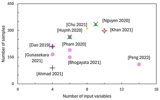
Figure 1.
Number of input variables of previous studies [23,30,31,43,44,45,46,47,48,49].
This study addresses these critical gaps by not only developing highly accurate ML-based predictive models but also explicitly translating these advanced results into a clear, practical, and directly usable empirical formula for estimating FAGC compressive strength. By performing comprehensive global sensitivity analysis, the interactions among key input variables, including component content and curing conditions, are uncovered to facilitate a deeper understanding of the underlying mechanisms influencing FAGC strength. In short, this study aims to bridge the existing gap between sophisticated predictive modelling and practical engineering applications, significantly enhancing the accessibility and interpretability of ML-based predictive modelling outcomes within the construction material sector.
2. Experimental Program
2.1. Data Collection and Arrangement
The dataset used in this study consists of 293 experimental data, with 9 input variables (e.g., mix proportions, sodium hydroxide concentration, and curing conditions) and one output (i.e., 28-compressive strength). FAGC specimens were produced through a range of concrete mixes with an extensive range of variation in mix proportions, sodium hydroxide molarity, curing temperature, and time, as shown in Table 1.

Table 1.
The range of parameters.
2.2. Materials
The components of FAGC were coal fly ash (CFA), sodium hydroxide (SH), sodium silicate (SS), coarse aggregates (CAgg), fine aggregates (FAgg), and additional water (Water). Coal fly ash, an industrial by-product from coal-fired power stations, was utilised as the primary aluminosilicate source for FAGC. This fly ash belongs to “class F”, with a density of 2500 kg/m3. The chemical compositions of the fly ash are provided in Table 2. Alkaline activator consisted primarily of sodium hydroxide (NaOH), prepared in various concentrations, ranging from 4 to 18 M, and sodium silicate (Na2SiO3 with 27.63% SiO2, 8.37% Na2O, and 64% H2O). The coarse aggregates used had a nominal maximum size of 10–20 mm, while the fine aggregates had a particle size distribution within the range of 0.075–4.75 mm. The densities of coarse and fine aggregates were 2700 kg/m3 and 2650 kg/m3, respectively.
Table 2.
Chemical composition of the fly ash.
2.3. Specimen Preparation and Testing
A total of 293 FAGC mixtures were produced using a systematic approach consistent with methods previously established by the authors [50]. After casting, specimens were subjected to a controlled curing process in a temperature-controlled oven, with curing temperatures varying from 40 °C to 120 °C and the duration ranging from 2 to 24 h. Compressive strength testing was then performed with a loading rate of 0.15 to 0.35 MPa/s after 28 days. The entire laboratory-based process is illustrated in the flow diagram shown in Figure 2.
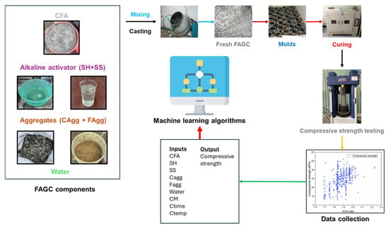
Figure 2.
Flow diagram of FAGC preparation, curing, and testing procedures.
3. Machine-Learning Modelling
3.1. Linear Regression
Linear regression [51] is a technique to estimate the relationship between input and output variables via a linear model (Equation (1)). Input variables are considered to be explanatory variables, while output variables are considered to be dependent variables. LR finds a best-fit hyperplane of dimension n − 1 to all observed points when the input dimension defines a space of dimension n.
A common method to find linear models is the least-squared method in which the linear model between dependent and explanatory variables is optimised by minimising the squared difference between target dependent values and predictions made by the linear model (Equation (2)).
A penalty on the size of the coefficients is also integrated to the optimisation equation (Ridge regression [52]) to control the complexity of the model (Equation (3)):
where α represents the complexity parameter and controls the complexity of the model.
3.2. Deep Neural Network
Deep neural network is a deep-learning architecture which utilizes the weight layers and activation functions to learn nonlinear representation of input features to best produce output. The basic component in DNN is perceptron, given in Figure 3. The collection of multiple perceptrons in layers with different selections of activation functions forms the network architecture to realise supervised learning tasks (e.g., regression and classification). Figure 4 represents a simple case of a DNN with 2 hidden layers. DNN is a feed-forward network with multiple network parameters finetuned by the gradient-based backpropagation algorithm [53]. Complex architectures with many nodes and layers expose DNN to the overfitting phenomenon, while simpler architectures have a high possibility of experiencing the underfitting phenomenon. Different additional techniques were designed to improve the learning performance of DNN’s parameters, such as optimisation methods (e.g., Adam [54], Adadelta [55], AdaMax, and Nadam [56]), L1 and L2 regularisation methods [57], normalisation methods (e.g., batch normalisation [58] and layer normalisation [59]), and other techniques (e.g., drop-out [60] and early stopping [61]). DNN architectures were used for practical regression problems in civil engineering, such as learning compressive strength of geopolymer concrete [30,62] and modelling strength of high-performance concrete [63,64,65,66], as well as predicting foamed concrete strength [67].
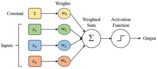
Figure 3.
Anatomy of a single node (perceptron) in DNN architecture.
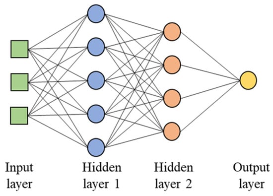
Figure 4.
A simple DNN architecture with 2 hidden layers.
3.3. Deep Residual Network
The deep residual network is a variation in the architecture of DNN, in which a skip connection from the input to the end of several stacked layers is inserted [68]. The ResNet architecture was first introduced for computer vision tasks to address the problem of gradient vanishing when training parameters for deep networks with many layers. The architecture was inherited and applied to the regression task of learning the compressive strength of fly ash-based geopolymer concrete, proving its advantage in providing a more accurate prediction model compared to the DNN-based model [30].
A normal DNN is trained to learn a function, F(X), where X is the inputs, while a ResNet aims to deliver a different function at output, i.e., H(X) = F(X) + X. As implemented in [30], the dimension of inputs may be different from the dimension of the last layer of F(X). Therefore, a modification was proposed in [68] that involved an additional layer for the skip connection to balance the dimensions of this connection and the part of stacked layers. Figure 5 represents a complete design of ResNet in this case where the number of nodes in Weight Layer 2 and Weight Layer 3 are identical to enable the function of the addition operator. In addition, normalisation methods are also included in the architecture to improve the learnability of ResNet architecture [30].
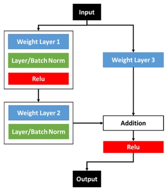
Figure 5.
Deep residual network (ResNet) architecture with an additional layer (Layer 3) to balance the dimension of skip connection and the layer prior to addition operator (Layer 2).
3.4. Sobol Sensitivity Analysis
Sobol analysis [69] is a global variance-based sensitivity analysis which analyses the extent to which the variance of input variables and their interactions affect the output variable. It considers prediction models as a “black box” function and provides a model-agnostic analysis approach to understand the sensitivity between input features and output features. Unlike local sensitivity analysis [70], which usually explores the sensitivity of the given set of input features, Sobol’s method offers a more holistic approach in which the effects of both input features and their interactions (at different orders, and total order relationship) on the sensitivity of the output are investigated. Sobol sensitivity analysis, therefore, provides more insights about the prediction models, but requires more data collection and computation resources than local approaches. Calculation of Sobol sensitivity score requires the calculation of expectation and variance of input variables and output variables. The first-order effect, the second-order effect, and the total-order effect of an input feature (xi) on output (Y) are measured by Equation (4), Equation (5), and Equation (6), respectively.
where Var(.) calculates the variance operator; E[:] is the expectation operator; l ∈ #i represents any set of variables, including input feature, xi; and Sl is calculated similar to Equation (5) for orders higher than two. An approximation method using Monte-Carlo sampling was also given in [69] to apply this method to practical models.
4. Empirical Framework Implementation
An empirical framework was established following a structured, three-stage procedure designed to achieve accurate and interpretable prediction of FAGC compressive strength, as shown in Figure 6. This framework was applied to a compiled database of 293 FAGC mixtures, with a broad range of mix proportions and curing conditions. The first stage focused on learning the most effective predictive relationship between input variables and output—compressive strength. The raw input features were pre-processed by using K-fold cross-validation, where the dataset was repeatedly split into training and validation parts. This pre-process step helps prevents overfitting and provides reliable estimates of the models’ performance. LR, DNN, and ResNet were implemented to build prediction models for FAGC strength. Each method offers distinct analytical strength. LR was selected due to its straightforward analytical and interpretability advantages, making it suitable as a baseline for comparing predictive capabilities. DNN was employed because of its powerful capacity to approximate complex nonlinear relationships between input variables and output [71]. ResNet was included for its advanced capability in handling intricate patterns in data by employing skip connections, overcoming potential performance degradation occurring often in deeper neural networks [72]. In this study, the same number of nodes was kept as 300 nodes and 200 nodes in Weight Layer 1 and Weight Layer 2, respectively. In the case of the ResNet model, an additional Weight Layer 3 with 200 nodes was added to ensure the feasibility of the element-wise addition operation at the end. The training and evaluation processes were carried out on the aforementioned datasets to systematically compare the predictive performance of these three approaches.
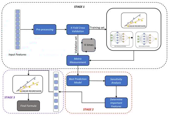
Figure 6.
Proposed framework to learn empirical formula for predicting FAGC compressive strength.
In the second stage, the interactions among input variables and their combined effect on FAGC strength were investigated using Sobol sensitivity analysis. Second-order effects were identified to understand the interactions between pairs of input variables. This provided crucial insight into previously unrecognised interdependencies, guiding the generation of a refined and enriched set of input variables. As illustrated in Figure 6, the best prediction model identified from stage 1 was used as the surrogate model for the Sobol analysis, and the results from Sobol sensitivity analysis were used to determine the most influential input features.
In the final stage, the newly identified and enhanced input features derived from Sobol sensitivity analysis were then incorporated into a subsequent linear regression model. The accuracy of the new formula obtained in this stage will be compared to the results obtained from the first stage. This final empirical formula aimed to enhance predictive accuracy while maintaining simplicity and interpretability.
5. Results and Discussions
5.1. Predictive Performance
Figure 7 presents the comparative performance of the three models (i.e., LR, DNN, and ResNet) in estimating the compressive strength of FAGC. The predicted values obtained from the ResNet model closely aligned with the experimental data, showing a better predictive accuracy compared to LR and DNN models. This is evident in both training and validation phases. Although the DNN model also shows considerable accuracy, its performance is slightly lower than that of ResNet. These findings align with previous studies [11,73], highlighting the capability of ResNet architectures in capturing complex, nonlinear relationships within the field of cementitious materials in general, and geopolymer concrete in particular.
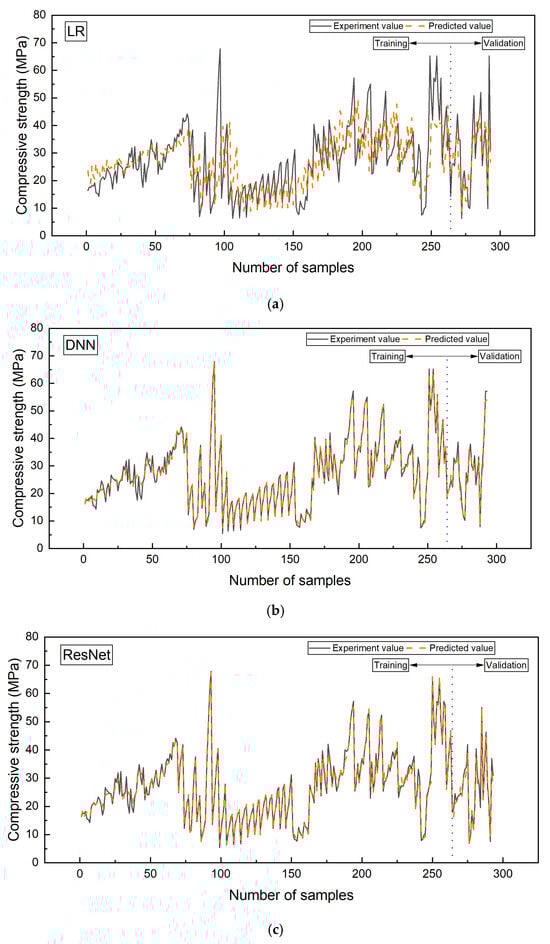
Figure 7.
Comparative performance of three predictive models: (a) LR, (b) DNN, and (c) ResNet.
Table 3 presents the predictive performance of the three models based on three error metrics, namely the coefficient of determination (R2), root mean-squared error (RMSE), and mean absolute error (MAE). These metrics were used for both training and validation datasets. As expected, ResNet and DNN consistently outperformed LR across all metrics. ResNet achieves the highest average validation R2 of 0.9108 and lowest RMSE and MAE (RMSE = 3.276; MAE = 2.3397), closely followed by DNN (R2 = 0.8963, RMSE = 3.5423, and MAE = 2.5363), whereas LR is at the lowest level (R2 = 0.6315, RMSE = 6.9529, and MAE = 5.3569). ResNet was reported to perform better than others because it can understand more complex patterns and make more accurate models [74,75]. While ResNet is commonly applied in image recognition and processing [76], its ability to model complicated patterns makes it suitable beyond purely visual tasks. In the case of geopolymer strength prediction, the underlying relationships among mix proportions, curing conditions, and mechanical behaviour are highly nonlinear and involve many interacting factors [77].
Table 3.
The predictive performance of three models based on three error metrics.
The radar charts in Figure 8 present the predictive performance of the three examined models, with simultaneous visualisation of multiple quantitative performance metrics (i.e., R2, RMSE, and MAE). While Table 3 provides precises statistical results, these radar charts enable a visual assessment of overall model balance with relative strength and weaknesses in prediction accuracy and stability. Overall, it is evident that ResNet and DNN both exhibit substantially better predictive accuracy compared to LR, with ResNet showing a slightly superior performance, as indicated by marginally higher R2 and lower RMSE and MAE values. The shaded transparent green and red regions represent the variability in performance across the 10-fold validation process. They also show the range between the maximum and minimum values for each metric. The narrower shaded area for the validation data compared to the training data indicates that the models exhibit consistent generalisation ability, with limited overfitting.
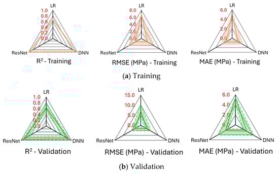
Figure 8.
Evaluation of the accuracy of the three predictive models: (a) training and (b) validation (R2, MAE, and RMSE).
5.2. Sensitivity Analysis
Figure 9 illustrates the sensitivity scores of first, second, and total order of FAGC, with nine input variables of the the models. It highlights the proportion of sodium silicate solution (SS), curing time (Ctime), SH molarity (CM), and water as the most critical inputs influencing FAGC compressive strength. First-order and total-order sensitivity scores from ResNet and the LR model show that Ctime is the most influential factor (29.1–34.5%), followed by WG (29.4–33.5%), while CAgg played the important role (30.4–41.6%) in FAGC strength from DNN’s model. As shown in the heatmap shown in Figure 9d–f, among the three models, ResNet and DNN captured significant nonlinearities and strong interactions, especially between the pair (SH and CAgg), with scores of 2.1–1.5%, whereas the LR (Figure 9a) model primarily identified linear relationships.
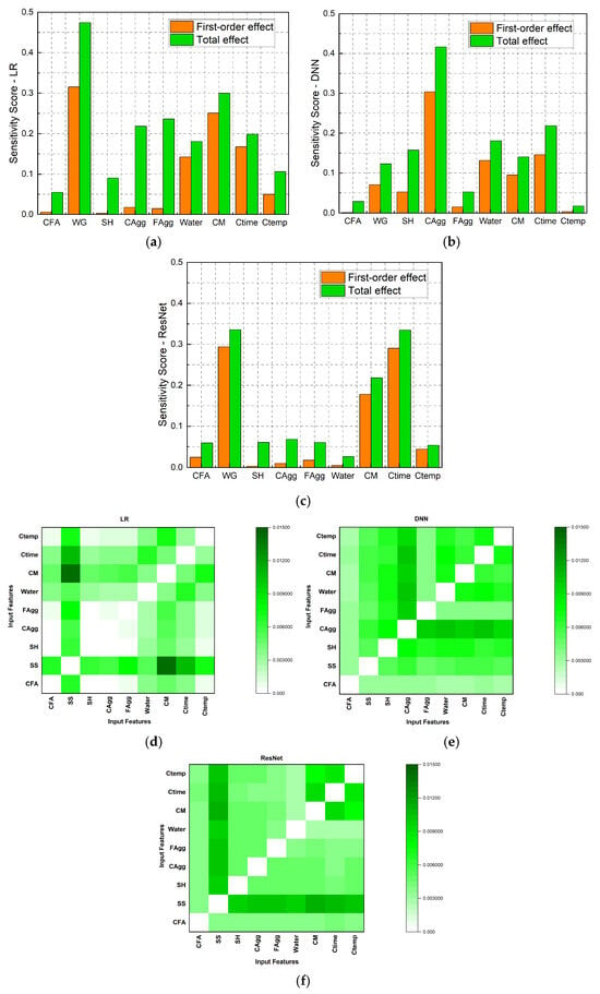
Figure 9.
Sensitivity analysis of the examined models (i.e., LR, DNN, and ResNet). (a–c) First-order and total-effect sensitivity scores. (d–f) Second-order sensitivity scores.
5.3. Proposed Empirical Models
Although the examined models show their ability to achieve high predictive accuracy, practitioners also need a fast, transparent tool for mix design, strength check, and day-to-day quality control. Empirical models meet this need by offering a closed-form relationship that can be inspected and deployed easily. In this study, multiple linear regression (MLR) was therefore selected as the predictive modelling technique due to its practicality and established effectiveness in estimating FAGC compressive strength [24]. While simple linear regression considers only one variable, MLR extends this approach to multiple independent variables being analysed simultaneously. This allows for a more accurate representation of the combined effects of different factors in FAGC mix design and curing conditions. The general form of the MLR equation is expressed as follows:
where is the 28-day compressive strength of FAGC; is the intercept; are the regression coefficients; and are the independent variables.
The proposed empirical model was built using the outcomes of global sensitivity analysis presented in Section 5.2. The top four most influential input variables were selected, which are sodium silicate solution (SS), curing time (Ctime), SH concentration molarity (CM), and water. Thus, Equation (7) becomes as follows:
Following the results obtained from Figure 9d, Equation (8) was re-constructed to include not only the four highest-ranking predictors from the base model (i.e., SS, Ctime, CM, and Water) but also two additional inputs that exhibited consistently high influence, i.e., fine aggregate content (FAgg) and curing temperature (Ctemp). The choice of six variables reflects a balance between model accuracy and complexity. This means reducing the set to lower than four might omit influential factors and degrade fit, while adding more than six variables might yield negligible incremental improvement. The newly re-constructed equation is expressed as follows:
The scatter plots illustrated in Figure 10 show the experimental versus predicted compressive strength of FAGC. Metric error RMSE was used to evaluate the performance of these models. As shown in Figure 10a, the four-input model yields an RMSE of 7.3697 (MPa) and shows noticeable dispersion, with a tendency to under-predict at strength between approximately 30 and 70 MPa, as many points fall below the line of equality. After adding the two inputs with high second-order sensitivity score, FAgg and Ctemp, to form the six-input model shown in Figure 10b, the scatter tightens, and more observations fall inside the ±20% error band, reducing RMSE to 6.8049 (MPa). This indicates a measurable improvement in predictive performance, particularly in the upper strength range.
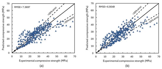
Figure 10.
Comparison between predicted and experimental compressive strength of FAGC: (a) with 4 inputs and (b) with 6 inputs.
6. Conclusions
This study presents a three-stage framework to build empirical formulae to forecast the compressive strength of fly ash-based geopolymer concrete. This framework integrates machine learning, global sensitivity analysis, and empirical modelling to achieve both predictive accuracy and practicality within a single systematic procedure. Based on the results of this study, the following key conclusions are as follows:
- ResNet model demonstrated the highest predictive accuracy among the models examined, confirming its suitability for modelling complex, nonlinear behaviour of FAGC. This indicates that deeper neural networks with skip connections work especially well for this type of geopolymer concrete.
- Global sensitivity analysis revealed that sodium silicate content, curing time, sodium hydroxide molarity, and water content have the greatest influence on FAGC compressive strength.
- The interaction between fine aggregate content and curing temperature was found to have a significant combined effect on FAGC strength, highlighting the importance of considering variable interactions in mix optimisation, rather than treating each mixture parameter in isolation.
- Empirical formulae that were developed based on the results from global sensitivity provide a practical and interpretable tool for predicting FAGC compressive strength with reduced computational demand, thus enabling efficient use in sustainable concrete design.
This framework demonstrates a systematic approach for translating a data-driven model into simple and practical predictive formulae. In this way, it connects advanced machine-learning models with simple design formulae and helps show which variables and interactions matter most for FAGC compressive strength. It can assist engineers and researchers in optimising mix proportions for specific performance targets and advancing the broader implementation of FAGC use in construction applications.
Author Contributions
Conceptualisation, T.-K.N. and T.-A.H.; methodology, T.-A.H.; software, V.-H.D.; validation, T.-K.N., A.A. and V.-H.D.; formal analysis, V.-H.D. and T.-A.H.; investigation, T.-K.N. and T.-A.H.; resources, T.-K.N. and T.-A.H.; data curation, V.-H.D.; writing—original draft preparation, T.-K.N. and T.-A.H.; writing—review and editing, T.-A.H. and A.A.; visualisation, T.-A.H. and A.A.; supervision, D.-K.T.; project administration, D.-K.T.; funding acquisition, D.-K.T. All authors have read and agreed to the published version of the manuscript.
Funding
This research received no external funding.
Data Availability Statement
The original contributions of this study are included in the article. Further inquiries can be directed to the corresponding author.
Conflicts of Interest
The authors declare no conflicts of interest.
Abbreviations
The following abbreviations are used in this manuscript:
| FAGC | Fly ash-based geopolymer concrete |
| LR | Linear regression |
| DNN | Deep neural network |
| ResNet | Residual neural network |
| OPC | Ordinary Portland cement |
| CO2 | Carbon dioxide |
| SiO2 | Silicon dioxide |
| Al2O3 | Aluminium oxide |
| SH | Sodium hydroxide |
| SS | Sodium silicate solution |
| SEM | Scanning electron microscope |
| XRD | X-ray diffraction |
| ANN | Artificial neural network |
| ML | Machine learning |
| ResNet | Deep residual network |
| CFA | Coal fly ash |
| RMSE | Root mean squared error |
| MAE | Mean absolute error |
| Ctime | Curing time |
| CM | SH molarity |
| CAgg | Coarse aggregate |
| FAgg | Fine aggregate |
References
- Davidovits, J. Geopolymers: Inorganic Polymeric New Materials. J. Therm. Anal. 1991, 37, 1633–1656. [Google Scholar] [CrossRef]
- Cheng, D.; Reiner, D.M.; Yang, F.; Cui, C.; Meng, J.; Shan, Y.; Liu, Y.; Tao, S.; Guan, D. Projecting Future Carbon Emissions from Cement Production in Developing Countries. Nat. Commun. 2023, 14, 8213. [Google Scholar] [CrossRef] [PubMed]
- Huang, L.; Li, B.; Zhu, X.; Li, N.; Zhang, X. Cement and Concrete as Carbon Sinks: Transforming a Climate Challenge into a Carbon Storage Opportunity. Carbon Capture Sci. Technol. 2025, 16, 100490. [Google Scholar] [CrossRef]
- Tkachenko, N.; Tang, K.; McCarten, M.; Reece, S.; Kampmann, D.; Hickey, C.; Bayaraa, M.; Foster, P.; Layman, C.; Rossi, C.; et al. Global Database of Cement Production Assets and Upstream Suppliers. Sci. Data 2023, 10, 696. [Google Scholar] [CrossRef]
- Cong, P.; Du, R.; Gao, H.; Chen, Z. Comparison and Assessment of Carbon Dioxide Emissions between Alkali-Activated Materials and OPC Cement Concrete. J. Traffic Transp. Eng. (Engl. Ed.) 2024, 11, 918–938. [Google Scholar] [CrossRef]
- Chan, C.C.S.; Thorpe, D.; Islam, M. An Evaluation Carbon Footprint in Fly Ash Based Geopolymer Cement and Ordinary Portland Cement Manufacture. In Proceedings of the 2015 IEEE International Conference on Industrial Engineering and Engineering Management (IEEM), Singapore, 6–9 December 2015; IEEE: New York, NY, USA, 2016; pp. 254–259. [Google Scholar]
- Setiawan, A.A.; Hardjasaputra, H.; Soegiarso, R. Embodied Carbon Dioxide of Fly Ash Based Geopolymer Concrete. IOP Conf. Ser. Earth Environ. Sci. 2023, 1195, 012031. [Google Scholar] [CrossRef]
- Ash, F.; Mayet, A.M.; Al-qahtani, A.A.; Mohammed, R.; Qaisi, A.; Ahmad, I.; Alhashim, H.H.; Eftekhari-zadeh, E. Developing a Model Based on the Radial Basis Function to Predict the Compressive Strength of Concrete Containing. Buildings 2022, 12, 1743. [Google Scholar] [CrossRef]
- Farhan, N.A.; Sheikh, M.N.; Hadi, M.N.S. Investigation of Engineering Properties of Normal and High Strength Fly Ash Based Geopolymer and Alkali-Activated Slag Concrete Compared to Ordinary Portland Cement Concrete. Constr. Build. Mater. 2019, 196, 26–42. [Google Scholar] [CrossRef]
- Al Bakri Abdullah, M.M.; Hussin, K.; Bnhussain, M.; Ismail, K.N.; Yahya, Z.; Razak, R.A. Fly Ash-Based Geopolymer Lightweight Concrete Using Foaming Agent. Int. J. Mol. Sci. 2012, 13, 7186–7198. [Google Scholar] [CrossRef]
- Emarah, D.A. Results in Materials Compressive Strength Analysis of Fly Ash-Based Geopolymer Concrete Using Machine Learning Approaches. Results Mater. 2022, 16, 100347. [Google Scholar] [CrossRef]
- Luan, C.; Shi, X.; Zhang, K.; Utashev, N.; Yang, F.; Dai, J. A Mix Design Method of Fly Ash Geopolymer Concrete Based on Factors Analysis. Constr. Build. Mater. 2021, 272, 121612. [Google Scholar] [CrossRef]
- Malkawi, A.B. Effect of Aggregate on the Performance of Fly-Ash-Based Geopolymer Concrete. Buildings 2023, 13, 769. [Google Scholar] [CrossRef]
- Parveen; Singhal, D.; Junaid, M.T.; Jindal, B.B.; Mehta, A. Mechanical and Microstructural Properties of Fly Ash Based Geopolymer Concrete Incorporating Alccofine at Ambient Curing. Constr. Build. Mater. 2018, 180, 298–307. [Google Scholar] [CrossRef]
- Singh Rajput, B.; Pratap Singh Rajawat, S.; Jain, G. Effect of Curing Conditions on the Compressive Strength of Fly Ash-Based Geopolymer Concrete. Mater. Today Proc. 2024, 103, 32–38. [Google Scholar] [CrossRef]
- Hassan, A.; Arif, M. Effect of Curing Condition on the Mechanical Properties of Fly Ash—Based Geopolymer Concrete. SN Appl. Sci. 2019, 1, 1694. [Google Scholar] [CrossRef]
- Verma, N.K.; Rao, M.C.; Kumar, S. Effect of Curing Regime on Compressive Strength of Geopolymer Concrete. IOP Conf. Ser. Earth Environ. Sci. 2022, 982, 012031. [Google Scholar] [CrossRef]
- Joseph, B.; Mathew, G. Influence of Aggregate Content on the Behavior of Fly Ash Based Geopolymer Concrete. Sci. Iran. 2012, 19, 1188–1194. [Google Scholar] [CrossRef]
- Assi, L.; Ghahari, S.; Deaver, E.; Leaphart, D.; Ziehl, P. Improvement of the Early and Final Compressive Strength of Fly Ash-Based Geopolymer Concrete at Ambient Conditions. Constr. Build. Mater. 2016, 123, 806–813. [Google Scholar] [CrossRef]
- Herwani; Pane, I.; Imran, I.; Budiono, B. Compressive Strength of Fly Ash-Based Geopolymer Concrete with a Variable of Sodium Hydroxide (NaOH) Solution Molarity. MATEC Web Conf. 2018, 147, 01004. [Google Scholar] [CrossRef]
- Naghizadeh, A.; Ekolu, S.O.; Tchadjie, L.N.; Solomon, F. Long-Term Strength Development and Durability Index Quality of Ambient-Cured Fly Ash Geopolymer Concretes. Constr. Build. Mater. 2023, 374, 130899. [Google Scholar] [CrossRef]
- Zhang, H.; Li, L.; Sarker, P.K.; Long, T.; Shi, X.; Wang, Q.; Cai, G. Investigating Various Factors Affecting the Long-Term Compressive Strength of Heat-Cured Fly Ash Geopolymer Concrete and the Use of Orthogonal Experimental Design Method. Int. J. Concr. Struct. Mater. 2019, 13, 63. [Google Scholar] [CrossRef]
- Gunasekara, C.; Atzarakis, P.; Lokuge, W.; Law, D.W.; Setunge, S. Novel Analytical Method for Mix Design and Performance Prediction of High Calcium Fly Ash Geopolymer Concrete. Polymers 2021, 13, 900. [Google Scholar] [CrossRef] [PubMed]
- Ahmed, H.U.; Mohammed, A.S.; Mohammed, A.A.; Faraj, R.H. Systematic Multiscale Models to Predict the Compressive Strength of Fly Ash-Based Geopolymer Concrete at Various Mixture Proportions and Curing Regimes. PLoS ONE 2021, 16, e0253006. [Google Scholar] [CrossRef] [PubMed]
- Kishore, Y.S.N.; Nadimpalli, S.G.D.; Potnuru, A.K.; Vemuri, J.; Khan, M.A. Statistical Analysis of Sustainable Geopolymer Concrete. Mater. Today Proc. 2022, 61, 212–223. [Google Scholar] [CrossRef]
- Saleh, P. Validation of Feret Regression Model for Fly Ash Based Geopolymer Concrete. Polytech. J. 2018, 8, 11. [Google Scholar] [CrossRef]
- Ali, A.A.; Al-Attar, T.S.; Abbas, W.A. A Statistical Model to Predict the Strength Development of Geopolymer Concrete Based on SiO2/Al2O3 Ratio Variation. Civ. Eng. J. 2022, 8, 454–471. [Google Scholar] [CrossRef]
- Bypour, M.; Yekrangnia, M.; Kioumarsi, M. Evaluation of the Compressive Strength of Fly Ash- Based Geopolymer Concrete Using Machine Learning. In The International Conference on Net-Zero Civil Infrastructures: Innovations in Materials, Structures, and Management Practices (NTZR); Springer Nature: Cham, Switzerland, 2025; pp. 801–811. [Google Scholar]
- Toufigh, V.; Jafari, A. Developing a Comprehensive Prediction Model for Compressive Strength of Fly Ash-Based Geopolymer Concrete (FAGC). Constr. Build. Mater. 2021, 277, 122241. [Google Scholar] [CrossRef]
- Nguyen, K.T.; Nguyen, Q.D.; Le, T.A.; Shin, J.; Lee, K. Analyzing the Compressive Strength of Green Fly Ash Based Geopolymer Concrete Using Experiment and Machine Learning Approaches. Constr. Build. Mater. 2020, 247, 118581. [Google Scholar] [CrossRef]
- Huynh, A.T.; Nguyen, Q.D.; Xuan, Q.L.; Magee, B.; Chung, T.; Tran, K.T.; Nguyen, K.T. A Machine Learning-Assisted Numerical Predictor for Compressive Strength of Geopolymer Concrete Based on Experimental Data and Sensitivity Analysis. Appl. Sci. 2020, 10, 7726. [Google Scholar] [CrossRef]
- Nia, M. Prediction of Compressive Strength of Fly Ash-Based Geopolymer Concrete Using Artificial Neural Network Model 1- Introduction. J. Adv. Inform. Water Soil Struct. 2025, 1, 98–114. [Google Scholar] [CrossRef]
- Ahmad, A.; Ahmad, W.; Aslam, F.; Joyklad, P. Compressive Strength Prediction of Fly Ash-Based Geopolymer Concrete via Advanced Machine Learning Techniques. Case Stud. Constr. Mater. 2022, 16, e00840. [Google Scholar] [CrossRef]
- Materials, B.; Khan, A.Q.; Naveed, H. Prediction of Compressive Strength of Fly Ash-Based Geopolymer Concrete Using Supervised Machine Learning Methods. Arab. J. Sci. Eng. 2024, 49, 4889–4904. [Google Scholar] [CrossRef]
- Verma, M. Prediction of Compressive Strength of Geopolymer Concrete Using Random Forest Machine and Deep Learning. Asian J. Civ. Eng. 2023, 24, 2659–2668. [Google Scholar] [CrossRef]
- Pazouki, G. Fly Ash-Based Geopolymer Concrete’s Compressive Strength Estimation by Applying Artificial Intelligence Methods. Measurement 2022, 203, 111916. [Google Scholar] [CrossRef]
- Biswas, R.; Kumar, M.; Kumar, D.R.; Samui, P.; Pradeep, T.; Rajak, M.K.; Armaghani, D.J.; Singh, S. Application of Novel Deep Neural Network on Prediction of Compressive Strength of Fly Ash Based Concrete. Nondestruct. Test. Eval. 2025, 40, 4638–4668. [Google Scholar] [CrossRef]
- Jin, S.; Zhao, Z.; Jiang, S.; Sun, J.; Pan, H.; Jiang, L. Comparison and Summary of Relevant Standards for Comprehensive Utilization of Fly Ash at Home and Abroad. IOP Conf. Ser. Earth Environ. Sci. 2021, 621, 012006. [Google Scholar] [CrossRef]
- Darmansyah, D.; You, S.-J.; Wang, Y.-F. Advancements of Coal Fly Ash and Its Prospective Implications for Sustainable Materials in Southeast Asian Countries: A Review. Renew. Sustain. Energy Rev. 2023, 188, 113895. [Google Scholar] [CrossRef]
- Tian, X.; Guo, Z.; Zhu, D.; Pan, J.; Yang, C.; Li, S. Recovery of Valuable Elements from Coal Fly Ash: A Review. Environ. Res. 2025, 282, 121928. [Google Scholar] [CrossRef]
- Mouawad, F.; Homsi, F.; Geara, F. Predicting Compressive Strength of Sustainable Concrete Using Machine Learning and Artificial Neural Networks. Constr. Mater. 2025, 5, 56. [Google Scholar] [CrossRef]
- Aichouni, M.; Messaoudene, N.A.; Touahmia, M.; Al-Ghonamy, A. Statistical Analysis of Concrete Strength Variability for Quality Assessment: Case Study of a Saudi Construction Project. Int. J. Adv. Appl. Sci. 2017, 4, 101–109. [Google Scholar] [CrossRef]
- Peng, Y.; Unluer, C. Analyzing the Mechanical Performance of Fly Ash-Based Geopolymer Concrete with Different Machine Learning Techniques. Constr. Build. Mater. 2022, 316, 125785. [Google Scholar] [CrossRef]
- Van Dao, D.; Ly, H.B.; Trinh, S.H.; Le, T.T.; Pham, B.T. Artificial Intelligence Approaches for Prediction of Compressive Strength of Geopolymer Concrete. Materials 2019, 12, 983. [Google Scholar] [CrossRef] [PubMed]
- Ly, H.B.; Le, T.T.; Vu, H.L.T.; Tran, V.Q.; Le, L.M.; Pham, B.T. Computational Hybrid Machine Learning Based Prediction of Shear Capacity for Steel Fiber Reinforced Concrete Beams. Sustainability 2020, 12, 2709. [Google Scholar] [CrossRef]
- Chu, H.-H.; Khan, M.A.; Javed, M.; Zafar, A.; Ijaz Khan, M.; Alabduljabbar, H.; Qayyum, S. Sustainable Use of Fly-Ash: Use of Gene-Expression Programming (GEP) and Multi-Expression Programming (MEP) for Forecasting the Compressive Strength Geopolymer Concrete. Ain Shams Eng. J. 2021, 12, 3603–3617. [Google Scholar] [CrossRef]
- Khan, M.A.; Zafar, A.; Farooq, F.; Javed, M.F.; Alyousef, R.; Alabduljabbar, H.; Khan, M.I. Geopolymer Concrete Compressive Strength via Artificial Neural Network, Adaptive Neuro Fuzzy Interface System, and Gene Expression Programming With K-Fold Cross Validation. Front. Mater. 2021, 8, 621163. [Google Scholar] [CrossRef]
- Bhogayata, A.; Kakadiya, S.; Makwana, R. Neural Network for Mixture Design Optimization of Geopolymer Concrete. ACI Mater. J. 2021, 118, 91–96. [Google Scholar] [CrossRef]
- Ahmad, M.; Rashid, K.; Tariq, Z.; Ju, M. Utilization of a Novel Artificial Intelligence Technique (ANFIS) to Predict the Compressive Strength of Fly Ash-Based Geopolymer. Constr. Build. Mater. 2021, 301, 124251. [Google Scholar] [CrossRef]
- Nguyen, K.T.; Le, T.A.; Lee, K. Evaluation of the Mechanical Properties of Sea Sand-Based Geopolymer Concrete and the Corrosion of Embedded Steel Bar. Constr. Build. Mater. 2018, 169, 462–472. [Google Scholar] [CrossRef]
- Freedman, D.A. Statistical Models: Theory and Practice; Cambridge University Press: Cambridge, UK, 2009; ISBN 9780521743853. [Google Scholar]
- Hoerl, A.E.; Kennard, R.W. Ridge Regression: Biased Estimation for Nonorthogonal Problems. Technometrics 2000, 42, 80–86. [Google Scholar] [CrossRef]
- Rumelhart, D.; Hinton, G.; Williams, R. Learning Representations by Back-Propagating Errors. Nature 1986, 323, 533–536. [Google Scholar] [CrossRef]
- Kingma, D.P.; Ba, J. Adam: A Method for Stochastic Optimization. arXiv 2014, arXiv:1412.6980. [Google Scholar]
- Zeiler, M.D. Adadelta: An Adaptive Learning Rate Method. arXiv 2012, arXiv:1212.5701. [Google Scholar] [CrossRef]
- Ruder, S. An Overview of Gradient Descent Optimization Algorithms. arXiv 2016, arXiv:1609.04747. [Google Scholar]
- Ng, A.Y. Feature Selection, L1 vs. L2 Regularization, and Rotational Invariance. In Proceedings of the Twenty-First International Conference on Machine Learning, Banff, AB, Canada, 4–8 July 2004; Association for Computing Machinery: New York, NY, USA, 2014. [Google Scholar]
- Ioffe, S.; Szegedy, C. Batch Normalization: Accelerating Deep Network Training by Reducing Internal Covariate Shift. Proc. Mach. Learn. Res. 2015, 37, 448–456. [Google Scholar] [CrossRef]
- Ba, J.L.; Kiros, J.R.; Hinton, G.E. Layer Normalization. arXiv 2016, arXiv:1607.06450. [Google Scholar] [CrossRef]
- Srivastava, N.; Hinton, G.; Krizhevsky, A.; Salakhutdinov, R. Dropout: A Simple Way to Prevent Neural Networks from Overfitting. J. Mach. Learn. Res. 2014, 15, 1929–1958. Available online: https://jmlr.org/papers/volume15/srivastava14a/srivastava14a.pdf (accessed on 14 December 2025).
- Caruana, R.; Lawrence, S.; Giles, L. Overfitting in Neural Nets: Backpropagation, Conjugate Gradient, and Early Stopping. Adv. Neural Inf. Process Syst. 2000, 13, 402–408. Available online: https://www.researchgate.net/publication/221620260_Overfitting_in_Neural_Nets_Backpropagation_Conjugate_Gradient_and_Early_Stopping (accessed on 21 December 2025).
- Dao, D.; Trinh, S.; Ly, H.-B.; Pham, B. Prediction of Compressive Strength of Geopolymer Concrete Using Entirely Steel Slag Aggregates: Novel Hybrid Artificial Intelligence Approaches. Appl. Sci. 2019, 9, 1113. [Google Scholar] [CrossRef]
- Yeh, I.-C. Modeling of Strength of High-Performance Concrete Using Artificial Neural Networks. Cem. Concr. Res. 1998, 28, 1797–1808. [Google Scholar] [CrossRef]
- Chou, J.-S.; Chiu, C.K.; Farfoura, M.; Al-Taharwa, I. Optimizing the Prediction Accuracy of Concrete Compressive Strength Based on a Comparison of Data-Mining Techniques. J. Comput. Civ. Eng. 2011, 25, 242–253. [Google Scholar] [CrossRef]
- Chou, J.S.; Pham, A.D. Enhanced Artificial Intelligence for Ensemble Approach to Predicting High Performance Concrete Compressive Strength. Constr. Build. Mater. 2013, 49, 554–563. [Google Scholar] [CrossRef]
- Qu, D.; Cai, X.; Chang, W. Evaluating the Effects of Steel Fibers on Mechanical Properties of Ultra-High Performance Concrete Using Artificial Neural Networks. Appl. Sci. 2018, 8, 1120. [Google Scholar] [CrossRef]
- Nguyen, T.; Kashani, A.; Ngo, T.; Bordas, S. Deep Neural Network with High-Order Neuron for the Prediction of Foamed Concrete Strength. Comput. Aided Civ. Infrastruct. Eng. 2019, 34, 316–332. [Google Scholar] [CrossRef]
- He, K.; Zhang, X.; Ren, S.; Sun, J. Deep Residual Learning for Image Recognition. arXiv 2015, arXiv:1512.03385. [Google Scholar] [CrossRef]
- Sobol, I.M. Global Sensitivity Indices for Nonlinear Mathematical Models and Their Monte Carlo Estimates. Math. Comput. Simul. 2001, 55, 271–280. [Google Scholar] [CrossRef]
- Li, D.; Jiang, P.; Hu, C.; Yan, T. Comparison of Local and Global Sensitivity Analysis Methods and Application to Thermal Hydraulic Phenomena. Prog. Nucl. Energy 2023, 158, 104612. [Google Scholar] [CrossRef]
- Elbrächter, D.; Perekrestenko, D.; Grohs, P.; Bölcskei, H. Deep Neural Network Approximation Theory. IEEE Trans. Inf. Theory 2021, 67, 2581–2623. [Google Scholar] [CrossRef]
- Zaeemzadeh, A.; Rahnavard, N.; Shah, M. Norm-Preservation: Why Residual Networks Can Become Extremely Deep? IEEE Trans. Pattern Anal. Mach. Intell. 2020, 43, 3980–3990. [Google Scholar] [CrossRef]
- Rathnayaka, M.; Karunasinghe, D.; Gunasekara, C.; Wijesundara, K.; Lokuge, W.; Law, D.W. Machine Learning Approaches to Predict Compressive Strength of Fly Ash-Based Geopolymer Concrete: A Comprehensive Review. Constr. Build. Mater. 2024, 419, 135519. [Google Scholar] [CrossRef]
- Shafiq, M.; Gu, Z. Applied Sciences Deep Residual Learning for Image Recognition: A Survey. Appl. Sci. 2022, 12, 8972. [Google Scholar] [CrossRef]
- Yun, C.; Jadbabaie, A. Are Deep ResNets Provably Better than Linear Predictors? Adv. Neural Inf. Process. Syst. 2019, 32, 22–29. Available online: https://proceedings.neurips.cc/paper_files/paper/2019/file/661c1c090ff5831a647202397c61d73c-Paper.pdf (accessed on 21 December 2025).
- Xu, W.; Fu, Y.-L.; Zhu, D. ResNet and Its Application to Medical Image Processing: Research Progress and Challenges. Comput. Methods Programs Biomed. 2023, 240, 107660. [Google Scholar] [CrossRef]
- Parhi, S.K.; Patro, S.K. Prediction of Compressive Strength of Geopolymer Concrete Using a Hybrid Ensemble of Grey Wolf Optimized Machine Learning Estimators. J. Build. Eng. 2023, 71, 106521. [Google Scholar] [CrossRef]
Disclaimer/Publisher’s Note: The statements, opinions and data contained in all publications are solely those of the individual author(s) and contributor(s) and not of MDPI and/or the editor(s). MDPI and/or the editor(s) disclaim responsibility for any injury to people or property resulting from any ideas, methods, instructions or products referred to in the content. |
© 2025 by the authors. Licensee MDPI, Basel, Switzerland. This article is an open access article distributed under the terms and conditions of the Creative Commons Attribution (CC BY) license.