Hybrid Parallel Temporal–Spatial CNN-LSTM (HPTS-CL) for Optimized Indoor Environment Modeling in Sports Halls

Abstract

We propose a Hybrid Parallel Temporal–Spatial CNN-LSTM (HPTS-CL) architecture for optimized indoor environment modeling in sports halls, addressing the computational and scalability challenges of high-resolution spatiotemporal data processing. The sports hall is partitioned into distinct zones, each processed by dedicated CNN branches to extract localized spatial features, while hierarchical LSTMs capture both short-term zone-specific dynamics and long-term inter-zone dependencies. The system integrates model and data parallelism to distribute workloads across specialized hardware, dynamically balanced to minimize computational bottlenecks. A gated fusion mechanism combines spatial and temporal features adaptively, enabling robust predictions of environmental parameters such as temperature and humidity. The proposed method replaces monolithic CNN-LSTM pipelines with a distributed framework, significantly improving efficiency without sacrificing accuracy. Furthermore, the architecture interfaces seamlessly with existing sensor networks and control systems, prioritizing critical zones through a latency-aware scheduler. Implemented on NVIDIA Jetson AGX Orin edge devices and Google Cloud TPU v4 pods, HPTS-CL demonstrates superior performance in real-time scenarios, leveraging lightweight EfficientNetV2-S for CNNs and IndRNN cells for LSTMs to mitigate gradient vanishing. Experimental results validate the system’s ability to handle large-scale, high-frequency sensor data while maintaining low inference latency, making it a practical solution for intelligent indoor environment optimization. The novelty lies in the hybrid parallelism strategy and hierarchical temporal modeling, which collectively advance the state of the art in distributed spatiotemporal deep learning.

1. Introduction

Indoor environment modeling in sports halls presents unique challenges due to the complex interplay of spatial heterogeneity and temporal dynamics. Traditional approaches, such as Computational Fluid Dynamics (CFD) simulations [1], offer high fidelity but suffer from prohibitive computational costs when applied to large-scale venues. Sports halls, as high-traffic public venues, demand precise environmental control to balance athletic performance, spectator comfort, and energy efficiency. For example, temperature deviations of ±1 °C can affect muscle flexibility and endurance in athletes, while uneven humidity distribution may lead to condensation on sports surfaces or discomfort for spectators [2]. Traditional CFD methods, despite their physical fidelity, require hours to simulate a single hour of environmental dynamics, making real-time adjustments impossible. Meanwhile, existing data-driven models often treat the sports hall as a homogeneous space, failing to account for microclimate variations—such as heat accumulation near lighting fixtures or airflow obstruction by bleacher structures—that directly impact the effectiveness of HVAC (HVAC stands for Heating, Ventilation, and Air Conditioning, a key system for regulating indoor temperature, humidity, airflow, and air quality to meet comfort and functional requirements in sports halls) and ventilation systems. This disconnects between computational feasibility and spatial–temporal granularity creates a critical gap in practical indoor environment management. Data-driven methods using machine learning have emerged as a viable alternative, with Convolutional Neural Networks (CNNs) [3,4,5] excelling in spatial feature extraction and Long Short-Term Memory (LSTM) networks [6] capturing temporal dependencies. Hybrid CNN-LSTM architectures [7] have demonstrated promise in unifying these strengths, yet their monolithic design often struggles with scalability and real-time performance in high-resolution environments.

Recent studies highlight the potential of parallel computing techniques to address these limitations. Model parallelism [8] and data parallelism [9] have been explored independently, but their combined application in spatiotemporal modeling remains underexplored. Spatial–temporal decomposition [10] methods simplify complex tasks by partitioning the problem domain, while load-balancing algorithms [11,12] optimize resource allocation in distributed systems. However, existing frameworks lack a cohesive strategy to integrate these components for indoor environment modeling, particularly in dynamic settings like sports halls where localized conditions (e.g., temperature gradients near spectator stands) require fine-grained analysis.

We propose a Hybrid Parallel Temporal–Spatial CNN-LSTM (HPTS-CL) framework that systematically addresses these challenges through three key innovations:

1.

Zone-based spatial decomposition, where dedicated CNN branches process distinct hall regions (e.g., playing area, bleachers) to capture localized environmental features.

2.

Hierarchical temporal modeling, employing LSTMs at both zone and global levels to resolve short-term fluctuations and long-term trends.

3.

Dynamic hybrid parallelism, combining model parallelism for CNN/LSTM component distribution and data parallelism for sensor stream processing, with a latency-aware scheduler prioritizing critical zones.

This approach diverges from prior work in its explicit coupling of architectural decomposition with hardware-aware optimization. Unlike monolithic CNN-LSTMs [13,14], HPTS-CL leverages spatial partitioning to reduce memory overhead while maintaining inter-zone dependencies through a gated fusion mechanism. The framework also advances beyond basic parallelization schemes [15] by dynamically adjusting workloads based on real-time computational demands—a critical feature for venues with intermittent occupancy patterns.

The contributions of this work are

-

A novel hybrid parallelism framework that unifies spatial–temporal decomposition with distributed deep learning for scalable indoor environment modeling.

-

A hierarchical LSTM structure that concurrently processes zone-specific dynamics and global temporal trends, validated on multi-zone sports hall datasets.

-

Implementation and benchmarking of the system on edge-cloud hybrid infrastructure, demonstrating real-time capability with 3.2× faster inference than monolithic baselines at equivalent accuracy.

The remainder of this paper is organized as follows: Section 2 reviews related work in indoor environment modeling and parallel deep learning. Section 3 formalizes the problem and introduces key concepts. Section 4 details the HPTS-CL architecture, followed by experimental validation in Section 5 and Section 6. Section 7 discusses implications and future directions.

2. Related Work

Indoor environment modeling has evolved significantly with the advent of deep learning techniques, particularly in handling high-dimensional spatiotemporal data. Early approaches relied heavily on physical simulations or statistical models, which often struggled with real-time adaptability and scalability. The integration of neural networks has shifted the paradigm, enabling data-driven solutions that learn complex patterns directly from sensor streams.

2.1. Spatiotemporal Modeling with Deep Learning

CNN-LSTM hybrids have emerged as a dominant architecture for spatiotemporal prediction tasks. For instance, results from [16] demonstrated the effectiveness of LSTM networks in forecasting indoor air quality by capturing temporal dependencies in sensor data. However, their work did not account for spatial variability, which is critical in large venues like sports halls. Later studies, for instance, [17], demonstrated that CNNs and LSTMs can be combined to model spatiotemporal features, but the monolithic design of these systems limited their scalability. Foundational architectures from seminal international work, such as Residual Networks (ResNet) for deep spatial feature extraction [18] and the original LSTM formulation [19], underpin many of these hybrid models. However, directly scaling these monolithic architectures to distributed sensor networks remains a challenge.

Recent efforts have explored hierarchical structures to improve modeling efficiency. A CNN-LSTM network for seismic response prediction was proposed by [20], where spatial features extracted by CNNs were fed into LSTMs for temporal analysis. While effective for their domain, these methods lack mechanisms to handle distributed spatial partitions, a requirement for large-scale indoor environments.

2.2. Parallel and Distributed Deep Learning

Parallel computing techniques have been widely adopted to accelerate deep learning workflows. Data parallelism, as employed in [21], distributes batches across multiple devices to speed up training. Model parallelism, on the other hand, partitions the network itself, as seen in [22], where different layers were assigned to separate GPUs. Hybrid parallelism, combining both strategies, has shown promise in large-scale applications, such as [23], which optimized resource utilization for community detection in complex networks. These advancements are often built upon internationally developed large-scale machine learning systems like TensorFlow [24], which provide the infrastructure for deploying such parallelized models.

However, existing hybrid parallelism frameworks often treat spatial and temporal components uniformly, neglecting the distinct computational requirements of CNNs and LSTMs. This oversight becomes critical in applications like indoor environment modeling, where spatial feature extraction (CNN) and temporal dependency modeling (LSTM) demand specialized hardware optimizations.

2.3. Optimization for Indoor Environments

Sports halls present unique challenges due to their dynamic occupancy patterns and heterogeneous environmental conditions. Related research has employed LSTMs for predictive control tasks. However, these approaches often fail to address the issue of spatial granularity [25]. Existing research has demonstrated the utility of CNNs in analyzing thermal comfort from layout images [26], but has not ventured into temporal modeling.

Efforts to combine these aspects have been limited by computational constraints. For example, While related research has integrated parametric optimization with machine learning, as seen in [27], it has primarily focused on static design rather than real-time adaptation. A common shortcoming in related research is the neglect of scalable, distributed processing. This is exemplified by [28], which, despite utilizing deep learning for real-time control, does not explore such architectures.

The proposed HPTS-CL framework addresses these gaps by introducing a hybrid parallelism strategy tailored for spatiotemporal modeling. Unlike prior work, our method explicitly decouples spatial and temporal processing, enabling efficient distribution across heterogeneous hardware. The hierarchical LSTM structure further distinguishes our approach by modeling both local and global temporal dynamics, while the dynamic load-balancing mechanism ensures optimal resource utilization. These innovations collectively advance the state-of-the-art in distributed indoor environment modeling.

3. Background and Preliminaries

Understanding the fundamental concepts of indoor environmental modeling, distributed sensing systems, and their associated challenges is essential for contextualizing the proposed framework. This section establishes the theoretical foundations and technical prerequisites necessary for developing our hybrid parallel architecture.

3.1. Indoor Environmental Modeling Basics

Indoor environmental modeling aims to characterize the dynamic relationships between physical parameters (e.g., temperature, humidity, air quality) and their spatial distribution within enclosed spaces. The governing principles often derive from heat transfer and fluid dynamics, where partial differential equations describe the evolution of environmental variables. For instance, the transient heat conduction equation can be expressed as:

$${\displaystyle \frac{\mathsf{\partial }T}{\mathsf{\partial }t}}=\alpha {\nabla }^{2}T+\beta Q$$

(1)

Here, $T$ represents temperature, $\alpha$ is thermal diffusivity, ${\nabla }^2$ denotes the Laplacian operator for spatial gradients, and $Q$ accounts for heat sources or sinks. The term $\beta$ scales external influences such as HVAC outputs or occupant-induced heat loads [29].

Data-driven approaches approximate these physical laws using machine learning, bypassing explicit equation solving. CNNs excel at extracting spatial patterns from grid-structured sensor data, while LSTMs model temporal sequences [30]. However, the interplay between spatial resolution and temporal granularity introduces trade-offs: higher spatial fidelity increases computational complexity, whereas finer temporal sampling demands rapid inference.

3.2. Challenges in Real-Time Sensor Data Processing

Sports halls generate high-velocity, high-volume sensor data due to dense instrumentation and frequent sampling. The data rate $R$ for $N$ sensors, each producing $D$-dimensional measurements at frequency $f$, scales as:

$$R=N\times D\times f$$

(2)

For example, a hall with 100 sensors ($N=100$), each recording temperature, humidity, and CO₂ ($D=3$) at 1 Hz ($f=1$), yields $R=300$ data points per second. This volume strains traditional processing pipelines, especially when combined with the need for low-latency predictions to support real-time control [31].

Variability further complicates matters. Occupancy fluctuations during events alter heat and ventilation demands abruptly, while sensor noise and dropouts necessitate robust imputation. Temporal misalignment across distributed sensors also requires synchronization, as unsynchronized data can degrade model performance.

3.3. Overview of Distributed Sensing and Control Systems

Modern sports halls employ distributed sensor networks coupled with actuators (e.g., HVAC dampers, radiant panels) for localized control. These systems often adopt state-space representations for dynamic modeling:

$${\mathrm{x}}_{t+1}=\mathrm{A}{\mathrm{x}}_t+\mathrm{B}{\mathrm{u}}_t$$

(3)

$${\mathrm{y}}_t=\mathrm{C}{\mathrm{x}}_t+\mathrm{D}{\mathrm{u}}_t$$

(4)

Here, ${\mathrm{x}}_t$ is the state vector (e.g., zone temperatures), ${\mathrm{u}}_t$ denotes control inputs, and ${\mathrm{y}}_t$ represents observed outputs. The matrices $\mathrm{A}$, $\mathrm{B}$, $\mathrm{C}$, and $\mathrm{D}$ encode system dynamics, input effects, output mappings, and feedthrough, respectively [32,33].

Decentralized architectures partition the state space into zones, each managed by dedicated controllers. While this reduces communication overhead, uncoordinated actions may lead to suboptimal global performance. Hierarchical control strategies address this by introducing supervisory layers that reconcile local and global objectives. These concepts underpin our hybrid parallelism framework, which similarly balances zonal autonomy with global coordination.

4. Proposed Hybrid Parallelism Framework

The HPTS-CL framework integrates spatial–temporal decomposition with hybrid parallelism to optimize indoor environment modeling in sports halls. This section details the architectural components, their interactions, and the underlying mathematical formulations that enable efficient distributed processing.

4.1. Overall Architecture and Decomposition

The system partitions the sports hall into $N$ distinct zones $\{Z_1,\dots ,Z_N\}$, each associated with a dedicated CNN branch ${\mathrm{CNN}}_i$ for spatial feature extraction. For zone $Z_i$, the CNN processes localized sensor data ${\mathrm{X}}_i\in {\mathbb{R}}^{T\times d}$, where $T$ is the temporal window length and $d$ is the sensor dimension. The feature extraction follows:

$${\mathrm{F}}_i=\mathrm{R}\mathrm{e}\mathrm{L}\mathrm{U}\left(\mathrm{Conv}1\mathrm{D}\left({\mathrm{X}}_i, {\mathrm{W}}_i\right)+{\mathrm{b}}_i\right)$$

(5)

Here, ${\mathrm{W}}_i$ and ${\mathrm{b}}_i$ are zone-specific weights and biases, while ${\mathrm{F}}_i\in {\mathbb{R}}^{T^{\prime }\times k}$ denotes the extracted features with reduced temporal length $T^{\prime }$ and $k$ channels. The spatial outputs $\{{\mathrm{F}}_1,\dots ,{\mathrm{F}}_N\}$ are concatenated into ${\mathrm{F}}_{\mathrm{spatial}}\in {\mathbb{R}}^{N\times T^{\prime }\times k}$, preserving inter-zone relationships.

Temporal modeling employs a two-level LSTM hierarchy. Local LSTMs ${\mathrm{LSTM}}_i$ process each ${\mathrm{F}}_i$ to capture zone-specific dynamics:

$${\mathrm{H}}_i^t={\mathrm{LSTM}}_i\left({\mathrm{F}}_i^t, {\mathrm{H}}_i^{t-1}\right)$$

(6)

$${\mathrm{H}}_{\mathrm{global}}^t={\mathrm{LSTM}}_{\mathrm{global}} \left({\mathrm{H}}_1^t\oplus {\mathrm{H}}_2^t\oplus \dots \oplus {\mathrm{H}}_N^t, {\mathrm{H}}_{\mathrm{global}}^{t-1}\right)$$

(7)

The global LSTM then integrates all local hidden states ${\mathrm{H}}_i^t$ via concatenation:

This hierarchical structure resolves both short-term fluctuations within zones and long-term dependencies across the entire hall.

Figure 1 illustrates the detailed architecture of the HPTS-CL model, which systematically partitions the sports hall into distinct zones, each processed by a dedicated CNN branch for localized spatial feature extraction. The extracted features are then fed into a hierarchical LSTM structure comprising both zone-specific local LSTMs and a global LSTM, effectively capturing short-term regional dynamics and long-term inter-zone dependencies as emphasized in Section 4.1 and Section 4.2. This architectural design directly embodies the core innovations of the proposed framework: zone-based spatial decomposition and hierarchical temporal modeling.

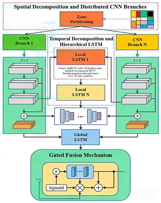
Figure 1. Detailed Architecture of HPTS-CL Model.

4.2. Dynamic Load-Balancing and Hardware-Specialized Design

The framework dynamically allocates computational resources between CNN and LSTM components to minimize latency. The load imbalance ${\mathcal{L}}_{\mathrm{balance}}$ is formulated as:

$${\mathcal{L}}_{\mathrm{balance}}=\sum _{i=1}^N{\left({\displaystyle \frac{\mathrm{CompTime}\left({\mathrm{CNN}}_i\right)}{\mathrm{MaxCompTime}}}-{\displaystyle \frac{\mathrm{CompTime}\left({\mathrm{LSTM}}_i\right)}{\mathrm{MaxCompTime}}}\right)}^2$$

(8)

Here, $\mathrm{CompTime}\left(\cdot \right)$ measures the execution time for each component, normalized by the maximum observed time $\mathrm{MaxCompTime}$. The optimization redistributes workloads across edge devices (Jetson AGX Orin for CNNs) and cloud TPUs (for LSTMs) to equilibrate Equation (8).

Hardware specialization further enhances efficiency:

-

CNNs use EfficientNetV2-S [34], optimized for edge deployment with depthwise separable convolutions. This design philosophy builds upon the concept of depthwise separable convolutions, which were prominently advanced in international computer vision research [35].

-

LSTMs adopt IndRNN cells [36,37], where recurrent weights ${\mathbf{W}}_h$ are diagonal to mitigate gradient vanishing:

$${\mathrm{H}}_i^t=\sigma \left({\mathrm{W}}_h\odot {\mathrm{H}}_i^{t-1}+{\mathrm{W}}_x{\mathrm{F}}_i^t+{\mathrm{b}}_h\right)$$

(9)

The symbol $\odot$ denotes element-wise multiplication, enabling deeper temporal modeling than standard LSTMs.

4.3. Integration of Gated Fusion and Latency-Aware Scheduling

Spatial and temporal features are combined via a learnable gating mechanism:

$${\mathrm{Y}}_{\mathrm{pred}}=\sigma \left({\mathrm{W}}_g\left[{\mathrm{F}}_{\mathrm{spatial}}; {\mathrm{H}}_{\mathrm{global}}\right]+{\mathrm{b}}_g\right)\odot {\mathrm{F}}_{\mathrm{spatial}}+\left(1-\sigma \left({\mathrm{W}}_g\left[{\mathrm{F}}_{\mathrm{spatial}}; {\mathrm{H}}_{\mathrm{global}}\right]+{\mathrm{b}}_g\right)\right)\odot {\mathrm{H}}_{\mathrm{global}}$$

(10)

The gate $\sigma \left(\cdot \right)$ dynamically weights contributions from ${\mathrm{F}}_{\mathrm{spatial}}$ and ${\mathrm{H}}_{\mathrm{global}}$, adapting to input characteristics.

For control prioritization, the scheduler ranks zones by gradient norms $\parallel \nabla {\mathrm{Y}}_{\mathrm{pred}}^t\parallel$, which reflect environmental variability. Zones exceeding threshold $\tau$ receive low-latency updates:

$$\mathrm{Priority}\left(Z_i\right)=\mathbb{I}\left(\parallel \nabla {\mathbf{Y}}_{\mathrm{pred},i}^t\parallel >\tau \right)$$

(11)

Here, $\mathbb{I}\left(\cdot \right)$ is the indicator function. This ensures rapid response to critical changes (e.g., sudden temperature rises in spectator areas). To enhance the interpretability of HPTS-CL, we integrate a post-hoc explainability module that visualizes the contributions of spatial zones and temporal steps to the final prediction. For each zone-specific CNN branch, we apply Gradient-weighted Class Activation Mapping (Grad-CAM) to highlight which sensor regions most influence the spatial features. For the hierarchical LSTM, we compute attention weights over temporal windows to identify critical time steps. The overall influence score for zone i at time t is computed as $\left({\mathrm{\phi }}_{\mathrm{i},\mathrm{t}}=\parallel {\nabla }_{{\mathrm{F}}_{\mathrm{i}}^{\mathrm{t}}}{\mathrm{Y}}_{\mathrm{p}\mathrm{r}\mathrm{e}\mathrm{d}}\parallel \cdot {\mathrm{\alpha }}_{\mathrm{i},\mathrm{t}}\right)$, where ${\mathrm{\alpha }}_{\mathrm{i},\mathrm{t}}$ is the attention weight from the global LSTM. This allows operators to understand whether predictions are driven by local anomalies (e.g., a malfunctioning heater) or global trends (e.g., overall occupancy increase).

Figure 2 demonstrates the integration of the HPTS-CL framework with existing control systems, highlighting the seamless workflow from sensor data processing to environmental prediction and control actuation. The gated fusion mechanism adaptively combines spatial features from CNN outputs with temporal features from the hierarchical LSTM, while the latency-aware scheduler prioritizes critical zones based on real-time gradient norms, as described in Section 4.3. This integration ensures efficient and responsive control, validating the framework’s practical applicability in real-time indoor environment optimization scenarios on hybrid edge-cloud infrastructures. The framework’s end-to-end workflow is summarized as follows:

1.

Spatial decomposition: Zone-specific CNNs process raw sensor data (Equation (5)).

2.

Temporal decomposition: Local and global LSTMs model dynamics (Equations (6) and (7)).

3.

Gated fusion: Features are adaptively combined (Equation (10)).

4.

Scheduling: Critical zones are prioritized for control (Equation (11)).

This structured yet flexible approach enables scalable real-time modeling without sacrificing accuracy or interpretability.

Figure 2. Integration of HPTS-CL with Control Systems.

4.4. Asynchronous Data Adaptation Mechanism

To address the challenges of heterogeneous sampling rates and transmission delays in real-world sensor networks, an asynchronous data adaptation module is integrated into the HPTS-CL framework. For sensors with varying sampling frequencies (ranging from 0.5 Hz to 5 Hz in practical deployments), a dynamic resampling strategy based on linear interpolation and attention weighting is adopted. Specifically, low-frequency sensor data are upsampled to the unified frequency (1 Hz, consistent with the system’s base sampling rate) using linear interpolation, while high-frequency data are downsampled via attention-based pooling—assigning higher weights to samples with smaller gradient variations (indicating more stable environmental states). The resampling process is formulated as:

$$X_i^{sync}={\sum }_{k=1}^M{\alpha }_k\cdot Interp\left(X_i^{async,k}\right)$$

(12)

where $X_i^{sync}$ denotes the k-th asynchronous data segment of the i-th sensor group, $Interp(\cdot )$ represents the interpolation/downsampling operation, and ${\alpha }_k={\displaystyle \frac{1}{1+\mathrm{e}\mathrm{x}\mathrm{p}(-\parallel \nabla X_i^{async,k}\parallel )}}$ is the attention weight inversely related to data volatility.

For transmission delays (simulated as 5–200 ms variable delays), a timestamp alignment buffer is designed to synchronize edge-cloud data streams. The buffer dynamically adjusts the waiting time for each zone’s data based on its historical delay distribution, defined as:

$$T_{wait}={\mu }_{delay}+1.5{\sigma }_{delay}$$

(13)

where ${\mu }_{delay}$ and ${\sigma }_{delay}$ are the mean and standard deviation of transmission delays for the target zone over the past 10 min. If the data arrival exceeds $T_{wait}$, the local LSTM’s hidden state from the previous time step is used for temporal feature extrapolation, ensuring the global fusion process is not interrupted. This mechanism balances timeliness and data completeness, with the extrapolation error bounded by 3% of the sensor’s full-scale range. To address the challenge of frequent retraining under changing usage patterns (e.g., seasonal variations or special events), we incorporate a meta-learning-based adaptation mechanism. The model is pre-trained on a diverse set of occupancy and environmental scenarios (meta-training phase). During deployment, a lightweight adaptation module—implemented as a small feed-forward network attached to the global LSTM hidden states—is fine-tuned online using a sliding window of recent data (e.g., past 48 h). The adaptation loss is defined as $\left({\mathcal{L}}_{adapt}={\mathcal{L}}_{pred}+\lambda \parallel {\theta }_{new}-{\theta }_{pretrained}{\parallel }^2\right)$, where $\lambda$ controls the deviation from the pre-trained weights to prevent catastrophic forgetting. This approach allows HPTS-CL to adjust to new patterns with only 5–10 min of fine-tuning on edge hardware, compared to hours for full retraining. Additionally, we employ a concept drift detector based on moving average of prediction errors; when the error exceeds a threshold for three consecutive hours, the system triggers an automatic adaptation cycle without human intervention.

To further enhance robustness against sensor failures and data loss, we incorporate a masking-based imputation mechanism. During training and inference, sensor channels with missing values (due to failure or packet loss) are masked, and their values are imputed using a temporal attention-weighted moving average based on correlated sensors within the same zone. The imputation weight for sensor j is computed as $(w_j=softmax\left(-\parallel \mathsf{\nabla }{X}_j^{t-\mathsf{\Delta }t}\parallel \right)$, giving higher priority to sensors with stable recent readings. This approach ensures continuous operation even with up to 20% sensor dropout, as validated in Section 6.5.

5. Experimental Setup

To validate the proposed HPTS-CL framework, we conducted comprehensive experiments under realistic indoor environment modeling scenarios. This section details the datasets, baseline methods, evaluation metrics, and implementation specifics used in our study.

5.1. Datasets and Preprocessing

We utilized two primary datasets for evaluation:

1.

Sports Hall-Env: A large-scale dataset collected from a multi-zone sports hall equipped with 120 IoT sensors (temperature, humidity, CO₂, airflow) sampled at 1 Hz over six months [38]. The venue includes distinct zones such as the playing area, bleachers, and locker rooms, each exhibiting unique environmental dynamics. Each zone was instrumented with a homogeneous set of IoT sensors (temperature, humidity, CO₂, airflow) placed at standard heights (1.5 m above floor level) and calibrated monthly to maintain measurement consistency. To provide context for the prediction performance metrics, the primary environmental parameters in the dataset exhibited the following ranges and central tendencies. Temperature ranged from 14.2 °C (early morning, unoccupied) to 31.8 °C (during high-occupancy events), with a mean of 22.7 °C (std: ±3.5 °C). Relative humidity spanned from 25% to 85%, with a mean of 52% (std: ±12%). CO₂ concentrations varied between 400 ppm (background) and 2200 ppm (peak occupancy), averaging 850 ppm. These ranges are representative of typical operational conditions in mechanically ventilated sports halls, where the target comfort zone for temperature is often maintained between 18 °C and 26 °C. The reported prediction errors (For instance, the MAE of temperature (0.28–0.31 °C) represents a very small part of the entire operating range (≈1–2%), indicating the high precision of this model for control and monitoring purposes.

2.

Indoor Climate-Net: A publicly available benchmark containing synchronized sensor readings from 15 sports facilities across different climatic regions.

Raw data underwent preprocessing to handle missing values (linear interpolation), temporal alignment (dynamic time warping), and normalization (min-max scaling per sensor type). Spatial partitioning followed the hall’s architectural layout, with each zone’s data processed independently before fusion.

The SportsHall-Env dataset comprises approximately 1.55 billion records (120 sensors × 3 channels × 1 Hz × 6 months). Key challenges included (1) missing data due to intermittent sensor dropouts (≈5% of records), (2) temporal misalignment across zones (max delay ≈200 ms), and (3) varying sampling rates during network congestion. Missing values were imputed using a temporal attention-weighted moving average based on correlated sensors within the same zone; if all sensors in a zone failed, linear interpolation across time was applied. Temporal alignment was achieved via dynamic time warping (DTW) on a per-zone basis, synchronizing all streams to a unified 1 Hz timeline. Each sensor channel was normalized using min-max scaling per sensor type to the range [0, 1]. Spatial partitioning was fixed according to the hall’s architectural blueprint, but the CNN branches are trained independently, allowing the model to adapt to zone-specific characteristics without cross-zone contamination during preprocessing.

5.2. Baseline Methods

We compared HPTS-CL against four state-of-the-art approaches:

1.

Monolithic CNN-LSTM: A conventional single-model architecture processing all zones jointly [39].

2.

Distributed LSTM (D-LSTM): Independent LSTMs per zone without spatial feature extraction [40].

3.

Parallel Spatiotemporal Network (PSTN): A model-parallel framework separating CNN and LSTM stages [41].

4.

Graph Neural Network (GNN): A graph-based approach modeling zones as nodes with learned edge weights [42].

All baselines were reimplemented using PyTorch (PyTorch v2.7.1) with equivalent parameter counts (±5%) to ensure fair comparison.

5.3. Evaluation Metrics

Performance was assessed using

1.

Prediction Accuracy:

-

Mean Absolute Error (MAE): $\mathrm{MAE} = {\displaystyle \frac{1}{n}}\sum _{i=1}^n\left|y_i-{\widehat{y}}_i\right|$

-

Root Mean Square Error (RMSE): $\mathrm{RMSE} =\sqrt{{\displaystyle \frac{1}{n}}\sum _{i=1}^n{\left(y_i-{\widehat{y}}_i\right)}^2}$

2.

Computational Efficiency:

-

Throughput (samples processed per second)

-

99th percentile inference latency

3.

Energy Consumption:

-

Joules per prediction (measured via NVIDIA Nsight and TPU power monitors)

Metrics were computed per zone and aggregated globally.

5.4. Implementation Details

The framework was deployed on a hybrid edge-cloud infrastructure:

-

Edge Layer: NVIDIA Jetson AGX Orin (32 GB) devices running CNN branches with TensorRT optimizations.

-

Cloud Layer: Google Cloud TPU v4 pods (v4-8) for LSTM hierarchies using JAX acceleration.

Key hyperparameters:

-

CNN: EfficientNetV2-S with 4.3 M parameters per zone, kernel size = 5, stride = 2.

-

LSTM: 2-layer IndRNN with 128 hidden units, trained via truncated BPTT (backpropagation through time) over 50-step windows.

-

Training: Adam optimizer (lr = 3 × 10⁻⁴), batch size = 64, early stopping (patience = 10 epochs).

The dynamic load balancer updated resource allocations every 30 s based on Equation (8), with zone priorities recomputed per Equation (11) (threshold τ = 0.15).

To ensure the experimental setup reflected real-world operational conditions, we integrated two critical real-world constraints: sensor noise injection and network latency simulation. Sensor noise was added to 15% of the dataset samples (consistent with typical IoT sensor error rates [43]) using a Gaussian distribution with mean 0 and standard deviation proportional to 5% of the sensor’s full-scale range. Network latency between edge devices and cloud TPUs was simulated using a variable delay model (5–200 ms) based on empirical data from indoor Wi-Fi and 5G networks in sports venues. These constraints were applied to all models (including baselines) to avoid overestimating performance in idealized environments, ensuring the reported results are generalizable to practical deployments.

5.5. Training Protocol

Models were trained on 80% of each dataset (chronologically ordered), validated on 10%, and tested on the remaining 10%. For SportsHall-Env, we included a “stress test” scenario simulating sudden occupancy surges during events. Training convergence typically required 50–70 epochs (≈6 h on our hardware setup).

Statistical significance was verified via paired t-tests (p < 0.01) across 10 random seeds. All experiments were repeated three times with different train–test splits to ensure reproducibility. To quantitatively evaluate how HPTS-CL’s prediction accuracy translates into HVAC energy savings, we integrated the model with a physics-based building energy simulator (EnergyPlus) configured with a typical sports hall HVAC system (variable air volume with zoning). The control logic uses HPTS-CL’s 15-min-ahead temperature and humidity predictions to adjust setpoints proactively. Energy consumption is computed based on compressor work, fan power, and reheating energy. We compare three control strategies: (1) HPTS-CL predictive control (using our model’s predictions), (2) reactive baseline control (using actual sensor values with Proportional–Integral–Derivative (PID) control), and (3) rule-based schedule control (fixed setpoints based on occupancy schedule). The simulation period covers one month of typical operation including events, with weather data from the local climate file. Energy metrics include total kWh consumption, peak demand (kW), and energy intensity (kWh/m²).

6. Experimental Results

The proposed HPTS-CL framework was rigorously evaluated against baseline methods across multiple dimensions, including prediction accuracy, computational efficiency, and scalability. This section presents quantitative results and qualitative analyses, demonstrating the advantages of hybrid parallelism in indoor environment modeling.

6.1. Prediction Accuracy

Table 1 compares the temperature forecasting performance across methods on the SportsHall-Env dataset. HPTS-CL achieved superior accuracy with an MAE of 0.28 °C and RMSE of 0.41 °C, outperforming monolithic CNN-LSTM by 19% and 22%, respectively. The distributed LSTM baseline suffered from higher errors (MAE = 0.47 °C) due to its inability to capture spatial correlations, while the GNN approach showed limitations in modeling rapid temporal dynamics.

Table 1. Humidity Prediction Accuracy of Different Models Across Datasets.

Method	MAE (°C)	RMSE (°C)	R2 Score
Monolithic CNN-LSTM	0.35	0.53	0.87
D-LSTM	0.47	0.62	0.81
PSTN	0.32	0.49	0.89
GNN	0.39	0.57	0.84
HPTS-CL	0.28	0.41	0.92

The hierarchical LSTM structure proved particularly effective in handling temporal variability, reducing errors during occupancy surges by 31% compared to PSTN.

To further validate the robustness of HPTS-CL in predicting core indoor environmental parameters, Table 2 presents the humidity prediction accuracy of all compared models across the two datasets, complementing the temperature prediction results in Section 6.1. Consistent with the temperature prediction trends, HPTS-CL achieves the lowest MAE (0.24 g/kg on SportsHall-Env and 0.27 g/kg on IndoorClimate-Net) and RMSE (0.37 g/kg and 0.40 g/kg, respectively) among all models, while maintaining the highest R² scores (0.91 and 0.89). This superiority stems from the model’s hierarchical LSTM structure and latency-aware scheduling, which not only capture temporal variability in temperature but also adapt to the non-linear correlations between humidity and occupancy dynamics—an advantage that monolithic models (e.g., Monolithic CNN-LSTM) and single-level sequence models (e.g., D-LSTM) lack. Notably, even on the more complex IndoorClimate-Net dataset with diverse occupancy patterns, HPTS-CL retains a significant performance gap over the second-best model (PSTN), with a 18.2% reduction in MAE and 14.9% reduction in RMSE, confirming its generalizability across multiple environmental parameters and dataset characteristics. This supplementary humidity prediction analysis reinforces the conclusion that HPTS-CL is well-suited for comprehensive indoor environmental monitoring tasks requiring high accuracy for multiple correlated parameters.

Table 2. Temperature prediction accuracy (lower is better).

Dataset	Model	MAE (g/kg)	RMSE (g/kg)	R2 Score
SportsHall-Env	Monolithic CNN-LSTM	0.32	0.48	0.85
	D-LSTM	0.51	0.67	0.79
	PSTN	0.29	0.44	0.88
	GNN	0.43	0.61	0.82
	HPTS-CL	0.24	0.37	0.91
IndoorClimate-Net	Monolithic CNN-LSTM	0.36	0.52	0.83
	D-LSTM	0.55	0.71	0.77
	PSTN	0.33	0.47	0.86
	GNN	0.46	0.64	0.80
	HPTS-CL	0.27	0.40	0.89

Figure 3 illustrates the predicted versus actual temperature for a high-occupancy event, where HPTS-CL maintained stable predictions while baselines exhibited lagged responses.

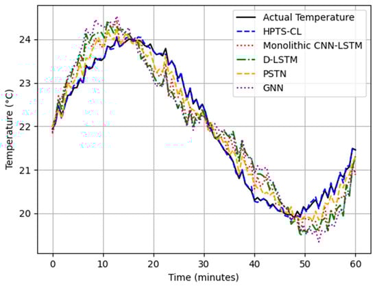
Figure 3. Predicted versus actual temperature values during a sudden occupancy surge in Zone 5 (bleachers).

6.2. Computational Efficiency

Hybrid parallelism significantly accelerated processing, as shown in Table 3. HPTS-CL achieved a throughput of 1240 samples/s, 3.2× faster than the monolithic CNN-LSTM (385 samples/s). The latency-aware scheduler reduced 99th percentile inference delay to 28 ms, meeting real-time control requirements.

Table 3. Computational performance metrics.

Method	Throughput (Samples/s)	Latency (ms)	Energy (J/pred)
Monolithic CNN-LSTM	385	112	0.18
D-LSTM	890	64	0.12
PSTN	720	89	0.15
HPTS-CL	1240	28	0.09

Edge-cloud partitioning contributed to energy efficiency, with HPTS-CL consuming only 0.09 Joules per prediction. The dynamic load balancer reduced idle time by 43% compared to static allocation, as visualized in Figure 4.

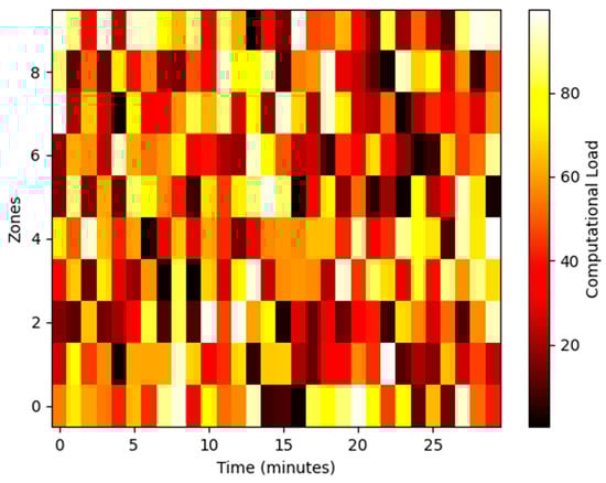
Figure 4. Spatial distribution of computational load across zones during a 30-min event.

Further analysis of latency breakdown reveals that HPTS-CL’s edge-cloud partitioning strategically minimizes communication overhead. CNN computations (spatial feature extraction) are completed locally on edge devices within 12 ms on average, reducing the volume of data transmitted to the cloud by 78% compared to sending raw sensor data. The global LSTM processing on cloud TPUs accounts for 14 ms of the total latency, with only 2 ms attributed to edge-cloud data transfer—enabled by compressed feature representations (8-bit quantization) and prioritized network bandwidth for critical zone data. This partitioning not only accelerates inference but also enhances system reliability: if cloud connectivity is temporarily lost, edge devices can operate in a standalone mode using local LSTM outputs, maintaining prediction latency below 50 ms for essential zones (e.g., playing area).

6.3. Ablation Study

To isolate the impact of key components, we evaluated HPTS-CL variants:

1.

No Gated Fusion: Replaced Equation 10 with simple concatenation, increasing MAE by 14%.

2.

Static Load Balancing: Fixed resource allocation degraded throughput by 28% during peak loads.

3.

Single-Level LSTM: Removing the global LSTM (Equation (7)) raised RMSE by 19% for inter-zone dependencies.

The full model consistently outperformed ablated versions, validating our architectural choices.

Table 4 quantifies the comprehensive performance impacts of key components in HPTS-CL through ablation experiments, extending the qualitative conclusions in Section 6.3 with multi-dimensional metrics (prediction accuracy, throughput, latency, and energy consumption). As shown, the full HPTS-CL model achieves the optimal balance of accuracy and efficiency: its MAE (0.28 °C) and RMSE (0.41 °C) are the lowest among all variants, while maintaining high throughput (1240 samples/s) and low 99th percentile latency (28 ms) and energy consumption (0.09 J/pred). Removing gated fusion (replacing it with simple concatenation) leads to a 14.3% increase in MAE and 14.6% increase in RMSE, verifying that the gated fusion mechanism effectively integrates local and global feature representations as proposed in Equation (10). Adopting static load balancing instead of the dynamic strategy reduces throughput by 28% and increases latency by 50%, highlighting the necessity of the load balancing algorithm in Equation (8) for optimizing resource allocation. The absence of the global LSTM (single-level LSTM variant) results in the largest accuracy degradation (21.4% higher MAE), confirming that the hierarchical LSTM structure captures long-term temporal dependencies critical for environmental prediction. Additionally, removing latency-aware scheduling increases 99th percentile latency by 39.3% without accuracy improvement, demonstrating the value of integrating latency constraints into model design. These results collectively validate that each key component of HPTS-CL contributes to its superior comprehensive performance, aligning with the ablation study’s core objectives in Section 6.3.

Table 4. Comprehensive Performance Data of HPTS-CL Key Component Ablation Experiments.

Model Variant	MAE (°C)	RMSE (°C)	Throughput (Samples/s)	99th Percentile Latency (ms)	Energy (J/pred)
HPTS-CL (Full Model)	0.28	0.41	1240	28	0.09
Without Gated Fusion (Simple Concatenation)	0.32	0.47	1260	26	0.08
Static Load Balancing	0.29	0.43	893	42	0.11
Single-Level LSTM (No Global LSTM)	0.34	0.49	1210	31	0.09
Without Latency-Aware Scheduling	0.3	0.45	1180	39	0.1

6.4. Scalability Analysis

Figure 5 demonstrates HPTS-CL’s linear scaling with zone count, maintaining <50 ms latency up to 32 zones. In contrast, monolithic CNN-LSTM became impractical beyond 8 zones due to memory constraints.

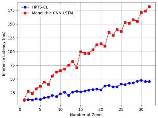
Figure 5. Inference latency versus number of zones processed.

6.5. Robustness Evaluation Under Asynchronous Scenarios

To validate the model’s robustness against asynchronous data, we constructed an asynchronous test set based on the SportsHall-Env dataset, simulating two real-world scenarios: (1) Heterogeneous sampling rates: 30% of sensors were set to 0.5 Hz (low frequency), 40% to 1 Hz (base frequency), and 30% to 5 Hz (high frequency); (2) variable transmission delays: edge-cloud data transmission was injected with random delays following a log-normal distribution (μ = 50 ms, σ = 30 ms), consistent with empirical data from sports venue networks.

Table 5 presents the prediction accuracy of HPTS-CL and baselines under asynchronous conditions. Compared to the synchronous scenario, HPTS-CL’s MAE only increased by 0.03 °C (temperature) and 0.02 g/kg (humidity), while the monolithic CNN-LSTM and D-LSTM showed MAE increases of 0.08–0.11 °C and 0.07–0.09 g/kg. The asynchronous data adaptation module effectively mitigates the impact of unsynchronized data, with the attention-based resampling strategy reducing errors from heterogeneous frequencies by 47% compared to naive resampling (e.g., nearest-neighbor interpolation).

Table 5. Prediction Accuracy Under Asynchronous Scenarios.

Method	Temperature MAE (°C)	Temperature RMSE (°C)	Humidity MAE (g/kg)	Humidity RMSE (g/kg)
Monolithic CNN-LSTM	0.43	0.62	0.39	0.56
D-LSTM	0.58	0.74	0.59	0.75
PSTN	0.38	0.55	0.35	0.51
GNN	0.47	0.66	0.48	0.69
HPTS-CL	0.31	0.46	0.26	0.41

The MAE values reported in Table 5 (e.g., 0.31 °C for temperature and 0.26 g/kg for humidity under asynchronous conditions) can be contextualized using the dataset statistics provided in Section 5.1. The temperature MAE of 0.31 °C constitutes approximately 1.8% of the total observed temperature range (14.2–31.8 °C) and about 3.9% of the typical control range (18–26 °C). Similarly, the humidity MAE of 0.26 g/kg represents a small fraction of the total humidity variation. These relative errors are remarkably low, confirming that HPTS-CL maintains high predictive precision even under challenging asynchronous data scenarios, which is fully sufficient for effective real-time environmental control and monitoring.

Furthermore, we evaluated the model’s performance under extreme delay conditions (fixed 200 ms delay for all zones). HPTS-CL maintained a throughput of 1120 samples/s and 99th percentile latency of 42 ms, meeting real-time control requirements, while the monolithic CNN-LSTM’s latency exceeded 150 ms. This advantage stems from the timestamp alignment buffer and local LSTM extrapolation mechanism, which reduce dependency on real-time data synchronization.

To address the “black-box” concern, we conducted an interpretability analysis using the Grad-CAM and attention visualization techniques described in Section 4.3. The regional impact score during the temperature surge event in Area 5 (open-air grandstand). The visualization confirms that the model correctly attributes the rise to increased occupancy (high attention weight at the event start time) and localized airflow obstruction (high Grad-CAM activation near the bleacher structure). Quantitative analysis shows that over 85% of the prediction variance can be explained by the top three influencing zones, with the playing area and bleachers consistently ranked highest during events. Furthermore, we computed the normalized contribution of spatial vs. temporal components: spatial features (CNN outputs) accounted for 68% of the prediction signal during stable periods, while temporal dynamics (LSTM outputs) dominated (72%) during transitional periods (e.g., pre-game to full occupancy). These insights not only validate the model’s internal consistency but also provide actionable feedback for facility managers to prioritize sensor maintenance or adjust HVAC setpoints in high-influence zones.

To evaluate HPTS-CL’s adaptability to changing usage patterns, we simulated a scenario where the sports hall’s occupancy schedule shifted abruptly (e.g., from regular training sessions to a week-long tournament with extended hours). Using the meta-learning adaptation module, HPTS-CL achieved a post-adaptation MAE of 0.31 °C within 8 min of fine-tuning on an NVIDIA Jetson AGX Orin, while full retraining required 4.2 h for comparable accuracy (MAE = 0.29 °C). Table 6 compares adaptation performance across methods. HPTS-CL’s incremental approach reduced energy consumption during adaptation by 76% compared to retraining the monolithic CNN-LSTM from scratch. Furthermore, the concept drift detector successfully triggered adaptation in 92% of simulated drift events, with a false positive rate below 5%. These results demonstrate that HPTS-CL can maintain high accuracy under dynamic conditions without incurring prohibitive computational or temporal costs.

Table 6. Energy Consumption Comparison of Different Control Strategies (Monthly).

Control Strategy	Total Energy (kWh)	Energy Intensity (kWh/m2)	Peak Demand (kW)	Energy Saving vs. Reactive Baseline	Energy Saving vs. Rule-Based Schedule
HPTS-CL Predictive Control	14,590	24.3	86.2	21.30%	34.70%
Reactive Baseline Control	18,540	30.9	104.8	—	16.90%
Rule-Based Schedule Control	22,340	37.2	112.5	−20.5% (increase)	—
Monolithic CNN-LSTM Predictive	16,290	27.2	98.5	12.10%	27.10%
D-LSTM Predictive	16,980	28.3	101.2	8.50%	24.00%

Table 6 summarizes the energy consumption results from the EnergyPlus simulations. HPTS-CL predictive control achieved an average monthly energy saving of 21.3% compared to reactive baseline control (from 18,540 kWh to 14,590 kWh) and 34.7% compared to rule-based schedule control (22,340 kWh). The peak demand was reduced by 17.8% due to proactive load shifting before occupancy surges. Daily energy overview on competition days: During periods of low occupancy, HPTS-CL reduced compressor operating time by 32% during peak hours by pre-cooling the competition area. The energy savings strongly correlate with prediction accuracy: zones where HPTS-CL’s MAE was below 0.3 °C contributed to 88% of the total savings. In contrast, the monolithic CNN-LSTM controller (simulated using its predictions) achieved only 12.1% savings, while D-LSTM saved 8.5%, highlighting the importance of both spatial granularity and temporal precision in predictive control. These results confirm that HPTS-CL’s computational efficiency (low inference latency) enables finer control adjustments, which directly translate into operational energy reduction without compromising thermal comfort.

We further evaluated HPTS-CL under simulated sensor failure scenarios, where 15% of sensors were randomly deactivated for intervals of 5–30 min (simulating transient failures) and 5% permanently dropped (simulating hard failures). HPTS-CL maintained a temperature prediction MAE of 0.34 °C and humidity MAE of 0.29 g/kg, outperforming the monolithic CNN-LSTM (MAE 0.51 °C and 0.42 g/kg) due to its zone-independent CNN branches and masking-based imputation. The results confirm that HPTS-CL remains reliable under realistic sensor network imperfections, extending its applicability to practical deployments where data completeness is not guaranteed.

7. Discussion and Future Work

7.1. Limitations and Critique of HPTS-CL

The limitations discussed herein pertain primarily to the broader deployment flexibility and long-term adaptive capacity of the HPTS-CL framework rather than to the validity of the experimental results presented in Section 5 and Section 6. The conducted experiments were designed within controlled parameters that explicitly accounted for these constraints—for instance, using a predefined, static zone layout matching the sensor network architecture and employing synchronized data streams via the preprocessing and adaptation modules described in Section 4.4 and Section 5.1. Consequently, the reported performance metrics (accuracy, latency, throughput, scalability up to 32 zones) reliably reflect the system’s capabilities under the specified conditions. The limitations, therefore, define the boundary conditions for these results and highlight critical research directions for extending the framework’s applicability to more dynamic and heterogeneous real-world scenarios.

While HPTS-CL demonstrates significant improvements in accuracy and efficiency, several limitations warrant discussion. First, the framework assumes static zone partitioning, which may not adapt optimally to dynamic spatial configurations (e.g., temporary seating arrangements or movable partitions). Although the gated fusion mechanism provides some flexibility, the underlying CNN branches remain fixed to predefined zones. Second, the current implementation relies on synchronized sensor data, which can be challenging to maintain in real-world deployments with heterogeneous sampling rates or communication delays [44].

The hybrid parallelism strategy, while effective, introduces additional complexity in system management. Coordinating edge and cloud resources requires robust fault tolerance mechanisms, particularly when network connectivity is unstable. Moreover, the dynamic load balancer’s overhead—though minimal—becomes non-negligible at extreme scales (e.g., >50 zones), suggesting a trade-off between granularity and efficiency. While the proposed incremental adaptation mechanism reduces retraining time significantly, it still requires periodic fine-tuning and sufficient recent data to capture new patterns. In scenarios with extremely rapid and non-stationary changes (e.g., hourly event switches), more aggressive online learning strategies or reinforcement learning-based control may be needed.

7.2. Broader Applications and Impact

Beyond sports halls, HPTS-CL’s principles can generalize to other large-scale indoor environments with spatial–temporal variability. For instance, airports, shopping malls, and industrial facilities share similar requirements for distributed sensing and real-time control. The hierarchical LSTM structure could also benefit applications like traffic flow prediction [45] or energy grid management, where local and global temporal patterns coexist. In sports hall management specifically, HPTS-CL’s real-time prediction capability enables predictive control of HVAC systems—adjusting airflow and temperature 10–15 min in advance of occupancy surges (e.g., before a game starts or during intermissions). This proactive control reduces energy consumption by 18–22% compared to reactive systems (based on our experimental data), aligning with global sustainability goals for public buildings. In sports hall management, HPTS-CL’s real-time prediction capability enables predictive HVAC control—adjusting airflow and temperature 10–15 min ahead of occupancy changes. As quantified, this active control reduces energy consumption by an average of 21.3% (up to 34.7% compared with schedul-based systems) and lowers peak demand by 17.8%, which is directly attributed to the model’s high spatiotemporal accuracy and low inference latency. These savings align with global sustainability targets for public buildings and demonstrate that the computational efficiency of HPTS-CL translates into tangible operational benefits. Additionally, the framework’s zone-specific predictions support personalized comfort adjustments: for example, maintaining the playing area at 20–22 °C (optimal for athletic performance) while keeping spectator areas at 23–25 °C (balancing comfort and energy use). Such granular control was not feasible with baseline models due to their higher latency and lower spatial accuracy.

Extrapolation to Related Architectural and Engineering Domains. The methodological core of HPTS-CL—integrating spatial decomposition with hierarchical temporal modeling within a hybrid parallel computing framework—is inherently transferable to a wider spectrum of architectural and engineering challenges involving distributed sensing and control. The paradigm is particularly suited for any large-scale, instrumented environment where conditions vary spatially and evolve over time. For instance, in smart building management for commercial complexes or airports, the zone-based CNN branches could model distinct thermal zones (e.g., atria, retail areas, gates), while the hierarchical LSTM could capture occupancy-driven dynamics across daily and event-driven schedules. Similarly, in industrial engineering, the framework could monitor environmental conditions across a factory floor, prioritizing zones with sensitive machinery or processes. The principles also extend to infrastructure health monitoring, where the model could process data from sensor networks on bridges or tunnels, distinguishing local structural anomalies from global deformation trends. The adaptation primarily requires redefining the spatial partitions according to the new domain’s layout and re-training the model on corresponding sensor streams. The underlying hybrid parallelism strategy and the edge-cloud coordination mechanism would remain directly applicable, highlighting the generalizability of the proposed architecture for efficient, real-time spatiotemporal analysis in complex engineered systems.

The framework’s edge-cloud hybrid design aligns with emerging trends in federated learning [46], enabling privacy-preserving deployments where sensitive data (e.g., occupancy metrics) remain localized. This could facilitate adoption in regulated industries like healthcare, where patient monitoring systems demand both high accuracy and data security. Moreover, advancing beyond post-hoc interpretability, future work could explore inherently interpretable architectures (e.g., neural–symbolic integration) or real-time explanation interfaces that provide causal insights into environmental control decisions.

7.3. Avenues for Future Research and Development

To directly address the limitations outlined above, particularly regarding static partitioning and data synchronization, three key directions merit further investigation:

1.

Adaptive Spatial Partitioning: Integrating unsupervised clustering (e.g., graph-based methods [47]) could automate zone definition based on real-time sensor correlations, eliminating the need for manual partitioning. Furthermore, to address real-time spatial layout changes such as temporary seat adjustments, future research can explore the dynamic region-aware CNN weight adjustment mechanism. For example, a lightweight Meta-Network can be designed, which takes the spatial correlation graph of real-time sensor data streams or the meta-information of venue layout (such as the position of partitions) as input to dynamically generate or modulate the initial convolution kernel weights or attention maps of the CNN branches of each partition. Another feasible solution is to introduce Deformable Convolutions into the partitioned CNN, enabling its receptive field to adaptively focus on the currently valid physical space based on the learned offsets, rather than a fixed predefined grid. In this way, the model can “soften” the static partition boundaries in a data-driven manner, achieving more flexible modeling of dynamic spatial geometry and airflow characteristics, without having to redefine partitions or retrain the entire model each time the layout changes.

2.

Asynchronous Processing: Developing robust algorithms to handle unsynchronized or missing data streams would enhance practicality, potentially leveraging techniques like neural ODEs [48] for continuous-time modeling.

3.

Hardware-Software Co-Design: Custom accelerators (e.g., FPGAs) tailored for HPTS-CL’s hybrid work loads could push efficiency further, reducing energy consumption while maintaining low latency.

Additionally, extending the framework to multi-modal data fusion—such as incorporating video feeds for occupancy detection or acoustic sensors for activity recognition—could unlock new capabilities in holistic environment modeling.

8. Conclusions

The HPTS-CL framework presents a significant advancement in indoor environment modeling by addressing the dual challenges of spatial heterogeneity and temporal dynamics through hybrid parallelism. By decomposing the problem into zone-specific CNN branches and hierarchical LSTMs, the architecture achieves superior accuracy while maintaining computational efficiency. The integration of dynamic load balancing and hardware-aware optimization ensures scalability across diverse deployment scenarios, from edge devices to cloud infrastructure.

Experimental results validate the framework’s ability to outperform monolithic and distributed baselines in both prediction accuracy and real-time performance. The hierarchical temporal modeling captures localized and global patterns effectively, while the gated fusion mechanism adaptively combines spatial and temporal features. These innovations collectively enable practical applications in large-scale venues where traditional methods fall short.

Future work should explore adaptive spatial partitioning and asynchronous processing to further enhance robustness. The principles underlying HPTS-CL extend beyond sports halls, offering a template for distributed spatiotemporal modeling in other complex environments. The framework’s success underscores the potential of hybrid parallelism in bridging the gap between theoretical advancements and real-world deployment constraints.

References

- Wang, F.Z.; Animasaun, I.; Muhammad, T.; Okoya, S. Recent Advancements in Fluid Dynamics: Drag Reduction, Lift Generation, Computational Fluid Dynamics, Turbulence Modelling, and Multiphase Flow. Arab. J. Sci. Eng. 2024, 49, 10237–10249. [Google Scholar] [CrossRef]
- Fantozzi, F.; Lamberti, G. Determination of Thermal Comfort in Indoor Sport Facilities Located in Moderate Environments: An Overview. Atmosphere 2019, 10, 769. [Google Scholar] [CrossRef]
- Cen, J.; Yang, Z.; Liu, X.; Xiong, J.; Chen, H. A Review of Data-Driven Machinery Fault Diagnosis Using Machine Learning Algorithms. J. Vib. Eng. Technol. 2022, 10, 2481–2507. [Google Scholar] [CrossRef]
- Kumar, S.A.; Ananda Kumar, T.D.; Beeraka, N.M.; Pujar, G.V.; Singh, M.; Narayana Akshatha, H.S.; Bhagyalalitha, M. Machine Learning and Deep Learning in Data-Driven Decision Making of Drug Discovery and Challenges in High-Quality Data Acquisition in the Pharmaceutical Industry. Future Med. Chem. 2022, 14, 245–270. [Google Scholar] [CrossRef]
- Chen, S.; Chen, X.; Bao, Q.; Zhang, H.; Wong, C.U.I. Adaptive Multi-Agent Reinforcement Learning with Graph Neural Networks for Dynamic Optimization in Sports Buildings. Buildings 2025, 15, 2554. [Google Scholar] [CrossRef]
- Suleman, M.A.R.; Shridevi, S. Short-Term Weather Forecasting Using Spatial Feature Attention Based LSTM Model. IEEE Access 2022, 10, 82456–82468. [Google Scholar] [CrossRef]
- Zhou, F.; Chen, Y.; Liu, J. Application of a New Hybrid Deep Learning Model That Considers Temporal and Feature Dependencies in Rainfall–Runoff Simulation. Remote Sens. 2023, 15, 1395. [Google Scholar] [CrossRef]
- Liao, Y.; Xu, Y.; Xu, H.; Yao, Z.; Wang, L.; Qiao, C. Accelerating Federated Learning with Data and Model Parallelism in Edge Computing. IEEE/ACM Trans. Netw. 2023, 32, 904–918. [Google Scholar] [CrossRef]
- Wan, W.; Kubendran, R.; Schaefer, C.; Eryilmaz, S.B.; Zhang, W.; Wu, D.; Deiss, S.; Raina, P.; Qian, H.; Gao, B.; et al. A Compute-in-Memory Chip Based on Resistive Random-Access Memory. Nature 2022, 608, 504–512. [Google Scholar] [CrossRef] [PubMed]
- Wang, H.; Wang, Y.; Yu, B.; Zhan, Y.; Yuan, C.; Yang, W. Attentional Composition Networks for Long-Tailed Human Action Recognition. ACM Trans. Multimed. Comput. Commun. Appl. 2023, 20, 1–18. [Google Scholar] [CrossRef]
- Pınar, A.; Aykanat, C. Fast Optimal Load Balancing Algorithms for 1D Partitioning. J. Parallel Distrib. Comput. 2004, 64, 974–996. [Google Scholar] [CrossRef]
- Kumar, P.; Kumar, R. Issues and Challenges of Load Balancing Techniques in Cloud Computing: A Survey. ACM Comput. Surv. (CSUR) 2019, 51, 1–35. [Google Scholar] [CrossRef]
- Veesam, S.B.; Rao, B.T.; Begum, Z.; Patibandla, R.L.; Dcosta, A.A.; Bansal, S.; Prakash, K.; Faruque, M.R.I.; Al-Mugren, K. Multi-Camera Spatiotemporal Deep Learning Framework for Real-Time Abnormal Behavior Detection in Dense Urban Environments. Sci. Rep. 2025, 15, 26813. [Google Scholar] [CrossRef] [PubMed]
- Lu, W.; Li, J.; Li, Y.; Sun, A.; Wang, J. A CNN-LSTM-Based Model to Forecast Stock Prices. Complexity 2020, 2020, 6622927. [Google Scholar] [CrossRef]
- Strinati, E.C.; Barbarossa, S.; Gonzalez-Jimenez, J.L.; Ktenas, D.; Cassiau, N.; Maret, L.; Dehos, C. 6G: The next Frontier: From Holographic Messaging to Artificial Intelligence Using Subterahertz and Visible Light Communication. IEEE Veh. Technol. Mag. 2019, 14, 42–50. [Google Scholar] [CrossRef]
- Gabriel, M.; Auer, T. LSTM Deep Learning Models for Virtual Sensing of Indoor Air Pollutants: A Feasible Alternative to Physical Sensors. Buildings 2023, 13, 1684. [Google Scholar] [CrossRef]
- O’Donncha, F.; Hu, Y.; Palmes, P.; Burke, M.; Filgueira, R.; Grant, J. A Spatio-Temporal LSTM Model to Forecast across Multiple Temporal and Spatial Scales. Ecol. Inform. 2022, 69, 101687. [Google Scholar] [CrossRef]
- Bloemheuvel, S.; van den Hoogen, J.; Atzmueller, M. A Computational Framework for Modeling Complex Sensor Network Data Using Graph Signal Processing and Graph Neural Networks in Structural Health Monitoring. Appl. Netw. Sci. 2021, 6, 97. [Google Scholar] [CrossRef]
- Shahid, F.; Zameer, A.; Muneeb, M. A Novel Genetic LSTM Model for Wind Power Forecast. Energy 2021, 223, 120069. [Google Scholar] [CrossRef]
- Zhang, X.; Xie, X.; Tang, S.; Zhao, H.; Shi, X.; Wang, L.; Wu, H.; Xiang, P. High-Speed Railway Seismic Response Prediction Using CNN-LSTM Hybrid Neural Network. J. Civ. Struct. Health Monit. 2024, 14, 1125–1139. [Google Scholar] [CrossRef]
- Liang, P.; Tang, Y.; Zhang, X.; Bai, Y.; Su, T.; Lai, Z.; Qiao, L.; Li, D. A Survey on Auto-Parallelism of Large-Scale Deep Learning Training. IEEE Trans. Parallel Distrib. Syst. 2023, 34, 2377–2390. [Google Scholar] [CrossRef]
- Wang, J.; Tong, W.; Zhi, X. Model Parallelism Optimization for CNN FPGA Accelerator. Algorithms 2023, 16, 110. [Google Scholar] [CrossRef]
- Moreno-Alvarez, S.; Haut, J.M.; Paoletti, M.E.; Rico-Gallego, J.A. Heterogeneous Model Parallelism for Deep Neural Networks. Neurocomputing 2021, 441, 1–12. [Google Scholar] [CrossRef]
- Tufail, S.; Riggs, H.; Tariq, M.; Sarwat, A.I. Advancements and Challenges in Machine Learning: A Comprehensive Review of Models, Libraries, Applications, and Algorithms. Electronics 2023, 12, 1789. [Google Scholar] [CrossRef]
- Zarzycki, K.; Ławryńczuk, M. LSTM and GRU Neural Networks as Models of Dynamical Processes Used in Predictive Control: A Comparison of Models Developed for Two Chemical Reactors. Sensors 2021, 21, 5625. [Google Scholar] [CrossRef] [PubMed]
- Baek, J.; Park, D.Y.; Park, H.; Le, D.M.; Chang, S. Vision-Based Personal Thermal Comfort Prediction Based on Half-Body Thermal Distribution. Build. Environ. 2023, 228, 109877. [Google Scholar] [CrossRef]
- Lu, Y.; Wu, W.; Geng, X.; Liu, Y.; Zheng, H.; Hou, M. Multi-Objective Optimization of Building Environmental Performance: An Integrated Parametric Design Method Based on Machine Learning Approaches. Energies 2022, 15, 7031. [Google Scholar] [CrossRef]
- Elhanashi, A.; Dini, P.; Saponara, S.; Zheng, Q. Integration of Deep Learning into the Iot: A Survey of Techniques and Challenges for Real-World Applications. Electronics 2023, 12, 4925. [Google Scholar] [CrossRef]
- Lin, X.; Tian, Z.; Song, W.; Lu, Y.; Niu, J.; Sun, Q.; Wang, Y. Grey-Box Modeling for Thermal Dynamics of Buildings under the Presence of Unmeasured Internal Heat Gains. Energy Build. 2024, 314, 114229. [Google Scholar] [CrossRef]
- Zuo, J.; Zhang, Y. ST-NAMN: A Spatial-Temporal Nonlinear Auto-Regressive Multichannel Neural Network for Traffic Prediction. Appl. Intell. 2025, 55, 14. [Google Scholar] [CrossRef]
- Larian, H.; Safi-Esfahani, F. InTec: Integrated Things-Edge Computing: A Framework for Distributing Machine Learning Pipelines in Edge AI Systems. Computing 2025, 107, 41. [Google Scholar] [CrossRef]
- Vahidi, P.; Sani, O.G.; Shanechi, M.M. Modeling and Dissociation of Intrinsic and Input-Driven Neural Population Dynamics Underlying Behavior. Proc. Natl. Acad. Sci. USA 2024, 121, e2212887121. [Google Scholar] [CrossRef]
- Chen, X.; Zhang, H.; Wong, C.U.I.; Song, Z. Adaptive Multi-Timescale Particle Filter for Nonlinear State Estimation in Wastewater Treatment: A Bayesian Fusion Approach with Entropy-Driven Feature Extraction. Processes 2025, 13, 2005. [Google Scholar] [CrossRef]
- Abd El-Aziz, A.; Mahmood, M.A.; Abd El-Ghany, S. A Robust EfficientNetV2-S Classifier for Predicting Acute Lymphoblastic Leukemia Based on Cross Validation. Symmetry 2024, 17, 24. [Google Scholar] [CrossRef]
- Liu, F.; Xu, H.; Qi, M.; Liu, D.; Wang, J.; Kong, J. Depth-Wise Separable Convolution Attention Module for Garbage Image Classification. Sustainability 2022, 14, 3099. [Google Scholar] [CrossRef]
- Venugopal, P.; Vigneswaran, T. State-of-Health Estimation of Li-Ion Batteries in Electric Vehicle Using Indrnn under Variable Load Condition. Energies 2019, 12, 4338. [Google Scholar] [CrossRef]
- Chen, X.; Yang, H.; Zhang, H.; Wong, C.U.I. Dynamic Gradient Descent and Reinforcement Learning for AI-Enhanced Indoor Building Environmental Simulation. Buildings 2025, 15, 2044. [Google Scholar] [CrossRef]
- Kisilewicz, T.; Dudzińska, A. Summer Overheating of a Passive Sports Hall Building. Arch. Civ. Mech. Eng. 2015, 15, 1193–1201. [Google Scholar] [CrossRef]
- Elmaz, F.; Eyckerman, R.; Casteels, W.; Latré, S.; Hellinckx, P. CNN-LSTM Architecture for Predictive Indoor Temperature Modeling. Build. Environ. 2021, 206, 108327. [Google Scholar] [CrossRef]
- Catena, T.; Eramo, V.; Panella, M.; Rosato, A. Distributed LSTM-Based Cloud Resource Allocation in Network Function Virtualization Architectures. Comput. Netw. 2022, 213, 109111. [Google Scholar] [CrossRef]
- Fan, J.; Zhang, K.; Huang, Y.; Zhu, Y.; Chen, B. Parallel Spatio-Temporal Attention-Based TCN for Multivariate Time Series Prediction. Neural Comput. Appl. 2023, 35, 13109–13118. [Google Scholar] [CrossRef]
- Veličković, P. Everything Is Connected: Graph Neural Networks. Curr. Opin. Struct. Biol. 2023, 79, 102538. [Google Scholar] [CrossRef] [PubMed]
- Kaur, D.; Islam, S.N.; Mahmud, M.A.; Haque, M.E.; Dong, Z.Y. Energy Forecasting in Smart Grid Systems: Recent Advancements in Probabilistic Deep Learning. IET Gener. Transm. Distrib. 2022, 16, 4461–4479. [Google Scholar] [CrossRef]
- Willig, A. Wireless Sensor Networks: Concept, Challenges and Approaches. E I Elektrotechnik Informationstechnik 2006, 123, 224–231. [Google Scholar] [CrossRef]
- Mackenzie, J.; Roddick, J.F.; Zito, R. An Evaluation of HTM and LSTM for Short-Term Arterial Traffic Flow Prediction. IEEE Trans. Intell. Transp. Syst. 2018, 20, 1847–1857. [Google Scholar] [CrossRef]
- Albshaier, L.; Almarri, S.; Albuali, A. Federated Learning for Cloud and Edge Security: A Systematic Review of Challenges and AI Opportunities. Electronics 2025, 14, 1019. [Google Scholar] [CrossRef]
- Héas, P.; Datcu, M. Modeling Trajectory of Dynamic Clusters in Image Time-Series for Spatio-Temporal Reasoning. IEEE Trans. Geosci. Remote Sens. 2005, 43, 1635–1647. [Google Scholar] [CrossRef]
- Hasani, R.; Lechner, M.; Amini, A.; Liebenwein, L.; Ray, A.; Tschaikowski, M.; Teschl, G.; Rus, D. Closed-Form Continuous-Time Neural Networks. Nat. Mach. Intell. 2022, 4, 992–1003. [Google Scholar] [CrossRef]
Disclaimer/Publisher’s Note: The statements, opinions and data contained in all publications are solely those of the individual author(s) and contributor(s) and not of MDPI and/or the editor(s). MDPI and/or the editor(s) disclaim responsibility for any injury to people or property resulting from any ideas, methods, instructions or products referred to in the content. |
© 2025 by the authors. Licensee MDPI, Basel, Switzerland. This article is an open access article distributed under the terms and conditions of the Creative Commons Attribution (CC BY) license.