Automated Image-to-BIM Using Neural Radiance Fields and Vision-Language Semantic Modeling

Abstract

This study introduces a novel, automated image-to-BIM (Building Information Modeling) workflow designed to generate semantically rich and geometrically useful BIM models directly from RGB images. Conventional scan-to-BIM often relies on specialized, costly, and time-intensive equipment, specifically if LiDAR is used to generate point clouds (PCs). Typical workflows are followed by a separate post-processing step for semantic segmentation recently performed by deep learning models on the generated PCs. Instead, the proposed method integrates vision language object detection (YOLOv8x-World v2) and vision based segmentation (SAM 2.1) with Neural Radiance Fields (NeRF) 3D reconstruction to generate segmented, color-labeled PCs directly from images. The key novelty lies in bypassing post-processing on PCs by embedding semantic information at the pixel level in images, preserving it through reconstruction, and encoding it into the resulting color labeled PC, which allows building elements to be directly identified and geometrically extracted based on color labels. Extracted geometry is serialized into a JSON format and imported into Revit to automate BIM creation for walls, windows, and doors. Experimental validation on BIM models generated from Unmanned Aerial Vehicle (UAV)-based exterior datasets and standard camera-based interior datasets demonstrated high accuracy in detecting windows and doors. Spatial evaluations yielded up to 0.994 precision and 0.992 Intersection over Union (IoU). NeRF and Gaussian Splatting models, Nerfacto, Instant-NGP, and Splatfacto, were assessed. Nerfacto produced the most structured PCs suitable for geometry extraction and Splatfacto achieved the highest image reconstruction quality. The proposed method removes dependency on terrestrial surveying tools and separate segmentation processes on PCs. It provides a low-cost and scalable solution for generating BIM models in aging or undocumented buildings and supports practical applications such as renovation, digital twin, and facility management.

1. Introduction

Aging buildings represent a major challenge in the global construction landscape, with a substantial share urgently requiring retrofitting and upgrades to comply with current performance and safety standards [1]. A significant portion of the built environment lacks reliable as-built documentation, a problem especially prevalent in aging residential and commercial buildings where original design drawings are often missing, inaccurate, or outdated [2]. The absence of precise as-built information could create serious challenges in carrying out building simulations, cost estimations, and renovation planning. To address this, more accurate and up-to-date digital models can be created. Overall, the practical applications of these models are energy retrofitting, facility management, post-disaster reconstruction, façade renovation, solar panel placement, and interior redesign, all of which rely on sufficiently detailed digital representations of existing buildings. These models not only enhance operational efficiency in facility management but also play a vital role in improving energy performance and supporting sustainability goals [3]. Without them, these processes become time-consuming, error-prone, and costly, often requiring extensive on-site measurements and manual reconstruction of building geometry.

In addition, the construction sector accounts for nearly 40% of global energy use and carbon emissions, and retrofitting the existing building stock is essential to achieve decarbonization and sustainability targets [4]. However, many aging buildings remain undocumented or poorly represented in digital form, limiting the ability of owners and facility managers to plan retrofits, monitor performance, and implement data-driven maintenance. Automating the generation of building models from imagery offers a practical pathway to accelerate digital transformation across the industry. It enables small firms and public agencies, often constrained by cost and technical expertise, to access up-to-date spatial data for energy analysis, facility management, retrofit and renovation planning. This shows the importance of application of digital workflows, especially when integrated with Artificial Intelligence (AI) techniques, which contribute not only to technical innovation but also to societal goals of reducing emissions, extending building life cycles, and improving safety and occupant comfort through better-informed decision-making [5].

To address these challenges and enhance the accessibility of digital modeling solutions, Scan-to-BIM has emerged as a workflow for capturing the geometry of physical structures using 3D scanning technologies and creating intelligent models within BIM software [6,7]. This approach is valuable for generating as-built BIM models of aging or repurposed buildings that lack original design documents [8]. The conventional Scan-to-BIM workflow consists of acquiring 3D PC data, analyzing and classifying building elements, and manually converting the segmented data into as-built BIM models [9,10,11]. However, despite its widespread adoption, this process remains labor-intensive and difficult to standardize [12]. As a result, recent research has increasingly focused on automating the segmentation and classification of PCs using Deep Neural Networks (DNN) algorithms to extract semantically segmented features along with their corresponding geometry to achieve a fully automated Scan-to-BIM workflow [12].

Although these approaches have advanced the scan-to-BIM reconstruction process, several challenges remain. Firstly, the degree of automation remains constrained, as the generation of high-quality 3D semantic and BIM models still depends on manual or semi-automated tasks in existing approaches [10,11,13]. Secondly, current modeling techniques do not fully utilize the semantic information embedded in PCs, as segmentation is performed after PC generation, missing valuable priors that could improve integration and geometric consistency [14,15]. Third, PCs, which are an essential data source for developing BIM models [16], are typically obtained through range-based techniques such as laser scanning (LiDAR) or image-based methods such as digital photogrammetry [17]. Despite their effectiveness, these methods present challenges in terms of cost, efficiency, and the need for post-processing [18,19]. At their current stage, both methods require post-processing of the generated point cloud to perform semantic segmentation of building elements and extract geometric information necessary for BIM modeling.

With the advancement of AI techniques, post-processing on PCs has improved classification and segmentation accuracy; however, it continues to pose challenges to automation in both range-based and image-based methods. Common issues include noise in raw data, structural incompleteness due to occlusions in scans [20], and difficulties detecting components on reflective or textureless surfaces [21]. In image-based methods, projection-based label transfer might lead to misalignment errors [22]. Moreover, both approaches involve high computational effort and manual intervention. A further limitation lies in the strong dependency on the quality and domain relevance of training data. Widely used 3D segmentation datasets such as S3DIS [23] exhibit non-uniform sampling, noise, and missing regions, which, despite enabling high point-wise semantic accuracy, can degrade object-level reconstruction fidelity [24]. Likewise, 2D datasets like ADE20K [25] and NYU Depth V2 [26] lack the architectural specificity and spatial coherence necessary for reliable BIM modeling, although they could be popular for general segmentation tasks [27].

For this reason and to maximize the potential of PCs, this study introduces a novel method that integrates NeRF and computer vision-language models to generate structured, segmented, and color-labeled PCs directly from images, after which the geometry of building elements is extracted and the BIM model is generated automatically. The proposed method addresses identified challenges by (1) automating the workflow, (2) embedding semantic labels during reconstruction to eliminate misalignment, avoid post-processing, reduce computational overhead, and mitigate scan-related issues, (3) removing dependence on LiDAR or photogrammetry to reduce cost and setup complexity, and (4) bypassing limitations of domain-specific 3D and 2D datasets by leveraging direct image-based labeling through large pretrained models. The proposed method is also experimentally evaluated using metrics that assess spatial precision, geometric consistency, and reconstruction performance across both interior and exterior datasets to validate its effectiveness for automated BIM generation.

This paper is organized as follows. Section 2 reviews existing studies and identifies the research gaps. Section 3, Methodology, outlines the integrated workflow for combining image segmentation, NeRF-based 3D reconstruction, and automated BIM modeling. Section 4, Results, provides quantitative evaluations of segmentation accuracy, spatial alignment, and reconstruction quality using multiple NeRF models. Section 5, Discussion, reflects on the implications of the findings, highlights the methodological contributions, and identifies remaining challenges and future directions. Finally, Section 6, Conclusion, summarizes the key outcomes and practical advantages of the proposed method.

2. Literature Review

The automated Scan-to-BIM process has significantly evolved through the integration of DNN-based methods over the past decade. This evolution has been driven by the need to process large-scale PCs efficiently, enhance semantic segmentation, and improve topological consistency in as-built BIM reconstruction. The following sections review the existing studies and identify research gaps, as well as key contributions that have advanced the Scan-to-BIM workflow through improvements in geometry-based, hybrid, and deep learning approaches.

2.1. Traditional Geometry-Based Approaches

Early Scan-to-BIM automation research focused on geometry-based techniques, using planar segmentation, topology rules, and shape detection to extract structural elements from PCs. Tang et al. [28] provided an early comprehensive review by classifying methods into geometric modeling, object recognition, and relationship modeling, while also identifying challenges such as manual intervention, noise, and occlusions. Xiong et al. [29] extended these efforts with a two-phase methodology that combined planar segmentation and voxelization to detect walls, floors, and ceilings, with visibility reasoning and shape estimation for semantic enrichment of detections.

As BIM adoption increased, semi-automated approaches emerged to reduce manual effort by combining rule-based methods with user intervention. Jung et al. [8] introduced a hybrid approach that integrated Random Sample Consensus (RANSAC)-based segmentation, grid-based filtering, and boundary tracing to extract architectural elements with subsequent human refinement. Volk et al. [10] reviewed BIM adoption technological limitations and highlighted that while laser scanning, photogrammetry, and automated object recognition have improved PCs processing, the conversion of unstructured PCs data into semantically rich BIM models remains a challenge.

Subsequent methods have integrated into machine learning or optimization algorithms to improve segmentation and topology in automated Scan-to-BIM workflows. For example, Croce et al. [30] proposed a semi-automatic approach that combines Machine Learning techniques, specifically the Random Forest, for semantic segmentation and classification of architectural elements in 3D point clouds. They utilized Rhino and Grasshopper, to reconstruct parametric models for H-BIM applications. Ochmann et al. [31] proposed a volumetric multi-story reconstruction method formulated as an integer linear programming problem, using RANSAC-based plane detection to identify structural surfaces and Markov clustering to group spatially related elements to enforce geometric and topological constraints. Bassier and Vergauwen [32] proposed an unsupervised method that detects different wall axis types (straight, curved, and polyline-based) and reconstructs wall connections using clustering, geometric feature extraction, and topology reconstruction to generate IFC-compliant BIM models. Rausch and Haas [33] proposed an automated parametric approach for updating the shape and pose of BIM elements using PCs. Their dyna-BIM method applies genetic algorithms and simulated annealing to align as-designed BIMs with as-built data. Additionally, Perez-Perez et al. [34] enhanced segmentation in complex environments by integrating Support Vector Machines for semantic classification with AdaBoost for geometric labeling and probabilistic graphical models. Their method refined the detection of planar and non-planar features while preserving semantic consistency throughout the automated reconstruction.

2.2. Deep Learning-Based Approaches

Recent advancements in PC processing have greatly improved the accuracy and efficiency of 3D reconstruction and segmentation, which benefits Scan-to-BIM applications. Large-scale annotated datasets like ScanNet [35] have enabled better deep learning models for scene understanding. Methods such as PointNet [36], PointCNN [37], and PointNeXt [38] have refined feature extraction and classification. SEGCloud [39] improved segmentation accuracy, and PointNetLK [40] advanced PCs registration. These developments laid the foundation for deep learning in Scan-to-BIM workflows to reduce manual effort and increase automation in as-built modeling.

Huan et al. [41] proposed GeoRec, a DNN for geometry-enhanced semantic 3D reconstruction. The model integrates a geometry extractor with deep learning to improve layout estimation, camera pose recovery, and object detection via three modules: room layout, object detection, and object reconstruction. Tang et al. [42] developed a hybrid approach combining deep learning with morphological operations and RANSAC-based plane detection. Their method classifies PCs into thirteen semantic categories, refines spatial relationships through Markov Random Field optimization, and uses grammar-based modeling to generate IFC-compliant BIM models.

Recent studies have further advanced Scan-to-BIM automation by enhancing DNN models, segmentation, and connectivity detection. Campagnolo et al. [43] developed a fully automated pipeline using DNN-based instance segmentation with BIM-Net++, a lightweight voxel-based Convolutional Neural Networks (CNN) designed for semantic segmentation that identifies architectural elements such as walls, floors, and roofs. Their method refines segmentation via RANSAC for planar and Density-Based Spatial Clustering of Applications with Noise (DBSCAN) for non-planar elements before BIM reconstruction. Wu et al. [44] presented FLKPP, a prototype that integrates neural networks with architectonic grammar for improved segmentation and reconstruction. Their method uses KPConv for 3D semantic segmentation, floor-layer preprocessing, and DNN-based line detection to generate 2D floor plan grids before reconstructing BIM elements like walls, doors, and columns. Drobnyi et al. [45] proposed a deep geometric neural network for connectivity detection, modeling spatial relationships through planar segmentation, region growing, and proximity-based clustering with a PointNeXt-based model for edge classification to automate digital twin construction. Mahmoud et al. [46] introduced a framework that first applies a deep learning model for PC segmentation, followed by room clustering using DBSCAN. Line detection via RANSAC extracts walls and major structural elements, while a Dynamo-based algorithm automates the parametric reconstruction of structured components like walls and floors. The framework achieved high accuracy in semantic segmentation and geometric reconstruction, which enhances the automation of Scan-to-BIM workflows.

2.3. Image-Based Approaches

In addition to the range-based Scan-to-BIM methods previously discussed, recent studies have investigated image-based workflows as cost-effective and accessible alternatives to LiDAR-based approaches. These methods typically utilize 2D RGB images captured through handheld devices or UAV. Semantic segmentation is performed using DNNs, after which 3D PCs are generated using photogrammetric techniques such as Structure-from-Motion (SfM) or Multi-View Stereo (MVS).

Han et al. [47] developed an indoor reconstruction method using LiDAR sensors and image-based MVS data. They applied DeepLabv3 for semantic segmentation, trained on the Cityscapes dataset and their own annotations. Their system reconstructed walls, floors, and ceilings. Similarly, Pantoja-Rosero et al. [20] aimed to automate the generation of Level of Detail (LOD3) building models, focusing on masonry structures, using SfM and DNN-based semantic segmentation. Their method combined SfM to generate sparse PCs and camera poses with TernausNet deep learning models to segment façade openings. Polyfit is used to create LOD2 models, which were upgraded to LOD3 by triangulating segmented openings into 3D space. The findings demonstrate that the pipeline effectively reconstructs LOD3 models.

In infrastructure-focused work, Saovana et al. [48] introduced a method called Point cloud Classification based on image-based Instance Segmentation (PCIS). This approach utilizes digital images processed through CNN to generate 2D masks, which are transformed into 3D masks using camera parameters from SfM. These masks classify PCs by projecting rays from camera positions through the masks to the PCs. The findings demonstrate that PCIS achieves high accuracy, with an F1-score of 0.96 for one-class classification and 0.83 for six-class classification. Puliti et al. [49] introduced a method combining infrared thermography and SfM to detect subsurface defects in building envelopes. They applied a segmentation algorithm using temperature-based sliding windows and edge detection to identify thermal anomalies. The method achieved IoU of 78% for the handheld IR camera test and 83% for the UAV-based IR camera test, along with an F1-score of 0.87 for both tests, demonstrating high accuracy in automated damage detection.

Studies have also paid attention to exterior and interior BIM reconstruction. For example, Yang et al. [50] proposed an image-based approach for automatic as-built BIM generation by reconstructing 3D facades and identifying surface materials. Using images from uncalibrated cameras, PCs are created via SfM, segmented with RANSAC, and analyzed through semantic reasoning to detect elements like walls and windows. Wong et al. [22] proposed an image-based Scan-to-BIM method for interior building reconstruction using handheld phone imagery. Their method integrates photogrammetry, semantic segmentation, projection, and geometry-based refinement. Frames were processed using SfM and MVS to create dense PCs, followed by RANSAC and DBSCAN for structural surface detection. YOLOv8, trained on the HBD dataset, was used to segment building components for 2D images. These semantic masks were projected onto the 3D PC using a pinhole camera model. Weighted voting improved label consistency, and boundary refinements addressed windows and doors. The final data was exported to Revit for automated BIM generation, achieving 100% recognition accuracy and a geometric error of 0.056 m.

2.4. Neural Radiance Field 3D Reconstruction

While existing image-based Scan-to-BIM methods have shown promising results, they typically depend on photogrammetry to reconstruct point clouds and then apply semantic labels through projection or manual mapping. This two-step process is often vulnerable to issues such as occlusions, noisy or incomplete geometry, and inaccurate label alignment, especially in complex indoor scenes with clutter, reflective surfaces, or textureless regions. To address these limitations, NeRF is explored in this research, which eliminates the need for intermediate point clouds and projection by directly learning a continuous volumetric representation from posed 2D images. NeRF enables a more integrated and robust workflow for view synthesis and geometry reconstruction and offers higher fidelity and resilience in challenging environments common to indoor BIM applications.

NeRF, introduced by Mildenhall et al. [51], marked a significant breakthrough in photorealistic view synthesis and 3D scene reconstruction. NeRF represents a static scene as a continuous volumetric function that maps five-dimensional inputs, comprising a 3D spatial location and a 2D viewing direction, to a color and volume density. This function is learned through a fully connected Multilayer Perceptron (MLP), which estimates view-dependent radiance and differential opacity at each sampled coordinate. By casting rays from virtual cameras through the scene and integrating predicted values using differentiable volume rendering, NeRF can generate novel views with remarkable visual fidelity from a sparse set of posed RGB images. It is capable of reconstructing fine geometry and complex lighting effects more efficiently than traditional mesh-based or voxel-based techniques. Unlike prior approaches that rely on discretized representations or require ground-truth 3D geometry, NeRF can be trained using only 2D images and camera intrinsics, which makes it a versatile tool for image-based scene reconstruction.

Building upon this foundation, advancements have been made to adapt NeRF for practical applications. Instant-NGP, proposed by Müller et al. [52], reduces training time and memory usage through multi-resolution hash encoding and a compact, fully fused MLP. This model enables near-real-time reconstruction. To improve robustness in real-world scenes with camera pose noise and variable lighting conditions, Nerfacto was introduced as part of the Nerfstudio framework by Tancik et al. [53]. It combines pose refinement, proposal sampling, and hash-based density fields to achieve stable reconstructions even in noisy or incomplete datasets conditions. Based on the 3D Gaussian Splatting technique introduced by Kerbl et al. [54], Splatfacto replaces volumetric grids and MLPs with differentiable 3D Gaussians. This representation supports direct optimization over Gaussian attributes such as position, opacity, and anisotropy. It achieves competitive visual quality and supports real-time rendering through tile-based rasterization.

These advancements highlight NeRF’s emerging potential as a foundation for the next generation of Scan-to-BIM methods, offering an alternative to conventional workflows that rely on physical scanning devices for geometric data acquisition. With recent improvements in speed, robustness, and output quality, NeRF models such as Instant-NGP, Nerfacto, and Splatfacto may facilitate BIM generation based on image-derived information. However, despite its technical potential, the integration of NeRF into Scan-to-BIM workflows remains largely unexplored.

Despite ongoing advancements, current Scan-to-BIM studies still follow a two-stage process: first generating PCs using scanning devices such as LiDAR or photogrammetry, then applying semantic segmentation in a separate post-processing step using deep learning models on the PCs. This can also be a fragmented process due to multiple tasks, increasing processing time, adding complexity, and constraining the level of automation achievable. This study aims to offer a workflow to avoid or minimize limitations through an automated image-to-BIM method presented in the following sections.

3. Methodology

This study introduces a four-phase method that converts 2D images into a BIM model by combining DNN, computer vision, and geometric processing techniques. As illustrated in Figure 1, the workflow includes: (1) multi-view image acquisition followed by object detection and segmentation, (2) 3D scene reconstruction, PCs generation, and feature extraction, (3) automated BIM modeling in Autodesk Revit, (4.1) evaluation of NeRF models (4.2) and validation of the proposed method through semantic, spatial, and geometric performance metrics using case studies.

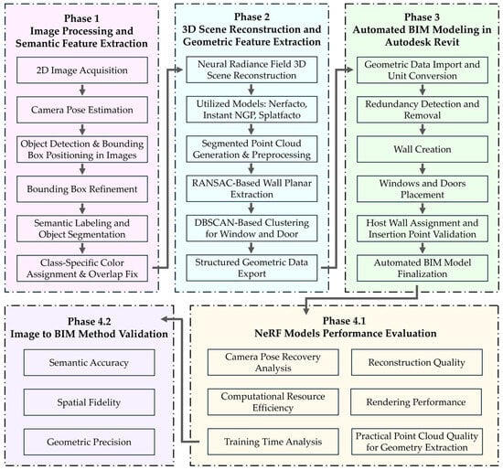
Figure 1. Proposed image-to-BIM method workflow from image input to automated BIM modeling.

3.1. Image Processing and Semantic Feature Extraction

3.1.1. Image Acquisition and Camera Pose Estimation

To reconstruct the scene accurately, images of the building from multiple angles are needed. The wider the coverage, the higher the quality of the NeRF reconstruction. In this study, two distinct real-world experimental case study datasets were used to evaluate the proposed method. One dataset consists of exterior images captured around the building, and the other consists of interior images captured from within the building to assess its performance in reconstructing both outdoor and indoor scenes.

Dataset 1 was collected from the exterior facades of an educational building in Turin, Italy. A UAV, the DJI Mini 4 Pro drone, capable of recording 4K video at 60 frames per second, captured the entire building exterior. The aerial survey generated high-resolution image frames with an effective resolution of 3840 × 2160 pixels, extracted from the recorded video stream. As shown in Figure 2, the UAV followed six flight paths at different altitude levels. Five rectilinear passes at heights of 2 m, 8 m, 14 m, 20 m, and 28 m, to have a complete façade coverage, while a final circular path at 38 m captured the upper structure and roof geometry. This structured survey provided a comprehensive dataset for the proposed image-to-BIM automation workflow.

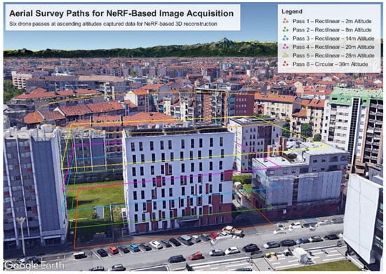
Figure 2. Aerial survey paths used for Dataset 1 image acquisition.

Dataset 2 was collected from the interior space of a room located in London. Unlike the UAV-based exterior survey, this dataset was acquired using a standard smartphone camera. A 60 s 4K video at a resolution of 3840 × 2160 pixels was recorded while walking through the room to capture the interior scene from multiple viewpoints.

Image frames were then extracted from the recorded video streams to construct the input datasets. To prepare the data for NeRF-based reconstruction, COLMAP was used to estimate camera poses and to output both the 3D coordinates of the camera positions and their corresponding viewing directions, which are essential for accurate NeRF training. As shown in Figure 3, the top-down view generated by COLMAP visualizes the confined indoor space, including the estimated camera poses and walking path.

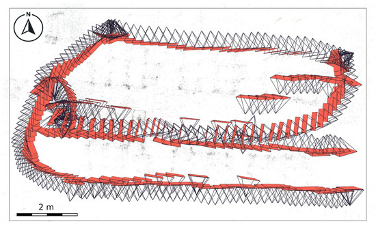
Figure 3. Top-down view of camera poses and walking path for Dataset 2.

3.1.2. Object Detection and Semantic Segmentation

After image acquisition, architectural elements were extracted through a process consisting of object detection, bounding box refinement, class-specific segmentation, and overlap resolution to first isolate only the building objects of interest (walls, windows, and doors in this study), and then apply color-labeled masks to those detected objects to prepare them for NeRF-based scene reconstruction. The embedded semantic information in the segmented images enabled the NeRF model to generate PCs in which each point inherits a class-specific color and preserves the identity of architectural elements throughout the reconstruction process.

The process began with object detection using YOLOv8x-worldv2 model, an open-vocabulary object detection model that uses CNN-based processing and vision-language pre-training [55]. The vision–language pre-training in YOLO-World enhances the model’s ability to detect objects by connecting image features and text embeddings. It performs open-vocabulary object detection using its pre-trained weights and enables recognition of new categories based on text prompts such as wall, window, or door [55]. This allows the model to detect architectural elements directly without additional retraining or fine-tuning on building-specific datasets. The model was employed to identify walls, windows, and doors within the input images and to generate bounding boxes annotated with class labels and confidence scores. Detection was performed using class-specific confidence thresholds to optimize accuracy for each object type. A lower threshold was applied for wall detection to maximize recall and broaden coverage, while higher thresholds were used for windows and doors to reduce false positives and improve precision. The model produced bounding boxes annotated with class labels and confidence scores. Following initial detection, redundant bounding boxes were filtered using a geometric merging strategy based on IoU calculations. Bounding boxes with IoU values exceeding 0.5 were merged to eliminate duplicates and to consolidate overlapping predictions into a single, unique representation per object.

The refined bounding boxes were then processed by an instance of the Segment Anything Model (SAM) 2.1, which is a computer vision model that employs a unified, prompt-based architecture to generate pixel-level segmentation masks in images [56]. Each bounding box served as a prompt for SAM to delineate the spatial extent of walls, windows, and doors. To visually encode semantic identity for subsequent NeRF-based reconstruction, predefined class-specific RGB values were applied. For Dataset 1, the segmentation masks used the following color scheme: walls in soft yellow (RGB: [220, 250, 50]), windows in green (RGB: [0, 255, 0]), and doors in blue (RGB: [0, 0, 255]). For Dataset 2, a distinct set of color codes was used: walls in red (RGB: [150, 50, 50]), windows in dark green (RGB: [0, 100, 0]), and doors in blue (RGB: [0, 0, 255]). In cases where objects overlapped in the 2D view, such as windows embedded in walls or doors positioned along edge boundaries, a hierarchical priority rule was applied. This rule resolved conflicts by assigning precedence to windows and doors over walls, to make sure that smaller embedded components were preserved and correctly labeled without being overridden by larger elements. Algorithm 1 outlines the full detection and segmentation workflow in pseudocode. Figure 4 shows an example transformation from a raw image to a segmented output, with each element clearly color-coded.

Algorithm 1: Object Detection and Segmentation

Input: Input image: $\mathit{I}$ Object detection model (YOLOv8x-worldv2): ${\mathit{M}}_{\mathit{Y}\mathit{O}\mathit{L}\mathit{O}}$ YOLO confidence thresholds: ${\mathit{\tau }}_{\mathit{o}}$, ${\mathit{\tau }}_{\mathit{w}}$ Bounding box merging IoU threshold: ${\mathit{\tau }}_{\mathit{I}\mathit{o}\mathit{U}}$ Predefined class labels and corresponding RGB colors: $\mathit{L}, {\mathit{C}}_{\mathit{R}\mathit{G}\mathit{B}}$ Segmentation model (SAM 2.1): ${\mathit{M}}_{\mathit{S}\mathit{A}\mathit{M}}$ Output: Segmented image: ${\mathit{I}}_{\mathit{s}\mathit{e}\mathit{g}}$

Initialize: Load $\mathit{I}, {\mathit{M}}_{\mathit{Y}\mathit{O}\mathit{L}\mathit{O}}, {\mathit{M}}_{\mathit{S}\mathit{A}\mathit{M}}, \mathit{L}, \mathbf{a}\mathbf{n}\mathbf{d} {\mathit{C}}_{\mathit{R}\mathit{G}\mathit{B}}$ Define function DetectObjects($\mathit{I}$$, {\mathit{\tau }}_{\mathit{o}}$$, {\mathit{\tau }}_{\mathit{w}}$$, {\mathit{M}}_{\mathit{Y}\mathit{O}\mathit{L}\mathit{O}}$): ○ Apply ${\mathit{M}}_{\mathit{Y}\mathit{O}\mathit{L}\mathit{O}}$ with confidence threshold ${\mathit{\tau }}_{\mathit{w}}$ for walls and ${\mathit{\tau }}_{\mathit{o}}$ for windows and doors objects detection. ○ Extract bounding boxes and class labels $\{\mathit{B},\mathit{C}\}$. ○ Return: Detected objects $\{\mathit{B},\mathit{C}\}$. End function Call DetectObjects ($\mathit{I}$$, {\mathit{\tau }}_{\mathit{o}}$$, {\mathit{\tau }}_{\mathit{w}}$$, {\mathit{M}}_{\mathit{Y}\mathit{O}\mathit{L}\mathit{O}}$): obtain detected elements $\{\mathit{B},\mathit{C}\}$. Define function MergeBoundingBoxes ($\{\mathit{B},\mathit{C}\}$$, {\mathit{\tau }}_{\mathit{I}\mathit{o}\mathit{U}}$): ○ For each pair of overlapping bounding boxes, compute IoU. ○ Merge boxes where IoU exceeds ${\mathit{\tau }}_{\mathit{I}\mathit{o}\mathit{U}}$. ○ Return: Refined bounding boxes {$\mathit{B}\mathit{\prime },\mathit{C}\mathit{\prime }$}. End function Call MergeBoundingBoxes ($\{\mathit{B},\mathit{C}\}$$,{\mathit{\tau }}_{\mathit{I}\mathit{o}\mathit{U}}$): refine detected elements $\{\mathit{B}\mathit{\prime },\mathit{C}\mathit{\prime }\}$. Define function SegmentObjects $\left(\mathit{I},{\{\mathit{B}}^{\mathit{\prime }},{\mathit{C}}^{\mathit{\prime }}\right\},{\mathit{M}}_{\mathit{S}\mathit{A}\mathit{M}},\mathit{L},{\mathit{C}}_{\mathit{R}\mathit{G}\mathit{B}})$: ○ For each bounding box in $\left\{{\mathit{B}}^{\mathit{\prime }},{\mathit{C}}^{\mathit{\prime }}\right\},$ apply ${\mathit{M}}_{\mathit{S}\mathit{A}\mathit{M}}$. ○ Assign predefined colors from ${\mathit{C}}_{\mathit{R}\mathit{G}\mathit{B}}$ to segmented elements based on $\mathit{L}$. ○ Apply hierarchical rules to resolve overlaps. ○ Return: Segmented image ${\mathit{I}}_{\mathit{s}\mathit{e}\mathit{g}}$. End function Call SegmentObjects $\left(\mathit{I},{\{\mathit{B}}^{\mathit{\prime }},{\mathit{C}}^{\mathit{\prime }}\right\},{\mathit{M}}_{\mathit{S}\mathit{A}\mathit{M}},\mathit{L},{\mathit{C}}_{\mathit{R}\mathit{G}\mathit{B}})$$: \mathrm{obtain} {\mathit{I}}_{\mathit{s}\mathit{e}\mathit{g}}$. Return: Segmented image ${\mathit{I}}_{\mathit{s}\mathit{e}\mathit{g}}$.

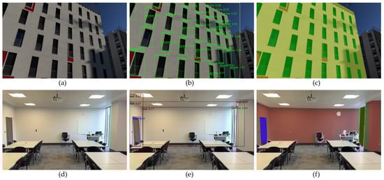
Figure 4. Transformation workflow illustrated using Dataset 1 (top) and Dataset 2 (bottom): (a,d) original images, (b,e) YOLO object detection results, and (c,f) SAM-generated segmentation masks.

3.2. Three-Dimensional Scene Reconstruction and Geometric Feature Extraction

3.2.1. Three-Dimensional Reconstruction Using Neural Radiance Fields

3D reconstruction models of Instant-NGP, Nerfacto, and Splatfacto were employed within the Nerfstudio framework to reconstruct the scenes from segmented images. Figure 5 illustrates NeRF reconstruction workflow applied on Dataset 1. In Figure 5a, semantically segmented images are used as multi-view inputs. These images are processed by COLMAP to estimate camera poses, shown in Figure 5b, where each triangle represents a viewpoint distributed around the building. Using the estimated poses and labeled RGB frames, NeRF constructs a scene-specific volumetric representation by casting rays from each camera location into the 3D scene, as depicted in Figure 5c. Along each ray, spatial samples are evaluated by a neural network to predict color and density. These predictions are integrated through differentiable volume rendering to reproduce the appearance of the input views. This process enables NeRF to learn a continuous function that maps 3D coordinates and viewing directions to radiance values, resulting in a high-fidelity, color-labeled 3D reconstruction of the building.

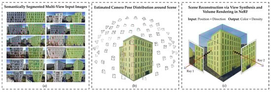
Figure 5. Illustration of the NeRF-based reconstruction workflow: (a) segmented image inputs, (b) estimated camera poses, and (c) volumetric rendering of the reconstructed 3D scene.

A distinguishing characteristic of NeRF methods is their optimization strategy. Unlike other DNN that aim to generalize across large datasets and avoid overfitting, NeRF models are intentionally overfitted to a single scene-specific dataset. This scene-specific optimization enables the model to learn fine-grained spatial and photometric details, resulting in high-fidelity volumetric representations tailored to the input scene.

To evaluate the impact of input data size on NeRF performance, a series of controlled experiments were conducted using subsets of the image dataset with increasing numbers of input frames. Specifically, NeRF models were trained on datasets comprising 50, 100, 150, 200, 250, 300, 350, 400, 500, and 550 images. This incremental sampling strategy allowed for a systematic assessment of how image quantity influences reconstruction quality, training stability, and PC quality. By varying the number of input views, the study aimed to identify thresholds beyond which additional data yield diminishing returns in terms of spatial completeness and semantic consistency in the reconstructed 3D scene. The results provide insights into optimal data requirements for different NeRF variants, particularly in the context of semantically segmented architectural environments.

In the proposed method, the segmentation labels embedded in the 2D images assist each NeRF model in aligning images from different viewpoints, leading to the generation of dense and color-encoded 3D PCs. The color information of each point corresponds directly to the segmentation labels, thereby preserving the identity of architectural elements in the reconstructed scene. Figure 6 demonstrates sample results of NeRF-based reconstruction using Nerfacto and segmented images produced by the proposed method.

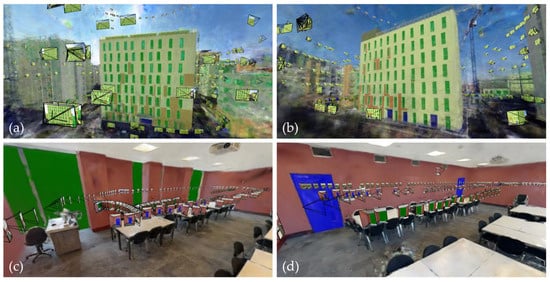
Figure 6. Nerfacto reconstruction outputs with embedded semantic information derived from 2D image segmentation for (a,b) Dataset 1 and (c,d) Dataset 2.

3.2.2. Point Clouds Preprocessing

The PCs generated from the NeRF reconstruction were preprocessed using Open3D 0.19.0 to optimize computational efficiency. Statistical outlier removal was applied to eliminate noise by discarding points that exhibited significant deviation from their local neighborhoods, thereby improving the overall quality and consistency of the data.

A voxel grid down-sampling algorithm with a 0.01 m voxel size is applied to reduce the point density and computational overhead while preserving structural details. The voxelization technique partitions the 3D space into discrete volumetric elements (voxels) and groups spatially adjacent points based on a fixed distance threshold. Seed points are iteratively selected, and neighboring points within the specified threshold are aggregated into clusters until the entire PC is organized into compact spatial groupings [57,58]. This method reduces the number of points in large-scale 3D scenes and maintains spatial detail and geometric continuity. It enables faster processing, reduces memory usage, and preserves the architectural integrity necessary for subsequent feature extraction. Figure 7 demonstrates PCs exported from the Nerfacto model for both exterior and interior datasets.

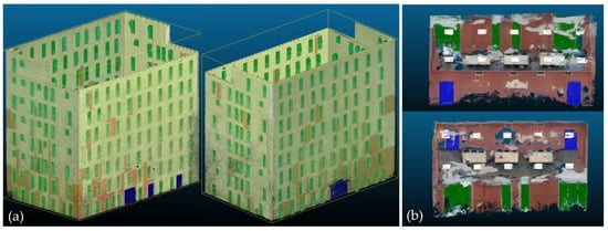
Figure 7. Extracted PCs from Nerfacto showing front and rear views for (a) Dataset 1, (b) Dataset 2.

3.2.3. RANSAC-Based Wall Planar Extraction

To extract wall features from the segmented PCs, a color-based filtering method is first applied. Since walls were pre-segmented with a yellow label in Dataset 1, a threshold-based filtering operation is used to isolate points where the red and green channels exceed 0.45, while the blue channel remains below 0.1. This selection method is utilized to retain only the wall regions and to reduce the influence of unwanted objects in the dataset. Following this, statistical outlier removal is performed using a neighborhood-based filtering approach, where points with fewer than 20 neighbors within a radius defined by a standard deviation ratio of 3.0 are discarded, to remove noise and isolate points.

To delineate wall geometries, RANSAC algorithm is employed for planar segmentation. RANSAC iteratively selects a random subset of points to fit a plane model, and classifies inliers that conform within a 0.3 m distance threshold while rejecting outliers. A maximum of 1000 iterations ensures that the model converges to an optimal planar representation of the walls. This iterative approach allows the detection of multiple wall planes and continues until either a predefined maximum number of walls is extracted or the remaining point count becomes insufficient for reliable plane fitting. Once planar segmentation is complete, a 2D line estimation is applied using Principal Component Analysis (PCA) on the XY coordinates of the inlier points. PCA is used to estimate the dominant direction of the wall segment, and the inlier points are projected onto this direction vector. The extreme projected points are designated as the start and end points of the wall. The wall height is determined from the minimum and maximum z-values of the inliers. Each wall is stored with its 2D direction vector, start and end points, base z-value, and height.

3.2.4. DBSCAN-Based Clustering for Window and Door Extraction

Following wall extraction, windows and doors are identified and isolated from the PCs using a color-based thresholding approach. The green channel is used to extract window points, where pixels with green intensity above 0.4 and low red and blue values are retained. Similarly, door points are extracted using a blue intensity threshold above 0.4, with low values in the other channels. This ensures that only the pre-segmented architectural elements are selected while unrelated objects are discarded.

To group these points into distinct architectural components, DBSCAN algorithm was employed. DBSCAN is suited for PCs clustering as it efficiently detects clusters of varying density and identifies outliers. The clustering parameters include eps = 0.32 and min_points = 60 for windows, and eps = 0.85 and min_points = 25 for doors. These values define the search radius and minimum cluster size and ensures that only significant and continuous structures are retained while filtering out noise. Figure 8 shows the PCs processing results, with walls extracted using RANSAC and windows and doors clustered using DBSCAN, represented by axis-aligned bounding boxes.

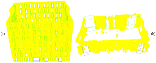
Figure 8. Point cloud processing results showing walls extracted using RANSAC and windows and doors clustered using DBSCAN with bounding boxes for (a) Dataset 1 and (b) Dataset 2.

Once clustering is complete, each detected window and door cluster is enclosed in an axis-aligned bounding box, which encapsulates the spatial extent of the object. Each bounding box stores key geometric attributes, including the center coordinates which represent the midpoint of the detected object, and the extent, which defines its width, height, and depth. Geometric attributes of each bounding box are used to assign window and door families and types, based on their correspondence to predefined Revit profiles.

To establish spatial relationships within the BIM model, each bounding box is assigned a host wall ID by computing the nearest wall based on the Euclidean distance between the bounding box center and detected wall planes. This ensures correct associations between extracted elements and their structural counterparts. Algorithm 2 illustrates the PCs Processing and Feature Extraction workflow in pseudocode.

3.2.5. Geometric Data Serialization in JSON Format

To facilitate BIM integration, the extracted geometric parameters from the PCs segmentation and clustering process are structured and serialized into a JSON file. This file serves as an intermediate data representation that preserves critical architectural information in a format that ensures compatibility with downstream automation workflows.

The JSON file is organized into three primary sections: “walls”, “windows”, and “doors”. Each wall entry includes a unique identifier, the 2D direction vector, the calculated start and end points, the base elevation, the measured wall height, and its orientation (horizontal or vertical). Similarly, each window and door entry contains a unique identifier, a reference to the host wall, and the bounding box parameters (center and extent), along with the object type label. By structuring the extracted data into a standardized JSON format, this approach enables automated data exchange between PCs, processing tools, and BIM platforms such as Autodesk Revit. Figure 9 illustrates the structure of the generated JSON file, showcasing how architectural features are serialized to enable seamless integration with the BIM model.

Algorithm 2: PCs Processing and Feature Extraction

Input: Segmented PCs and voxel size for down sampling: $\mathit{P}$, $\mathit{v}$ RANSAC distance threshold and maximum iterations for RANSAC: ${\mathit{\tau }}_{\mathit{d}}$, ${\mathit{n}}_{\mathit{m}\mathit{a}\mathit{x}}$ Maximum number of planes to detect: ${\mathit{m}}_{\mathit{m}\mathit{a}\mathit{x}}$ Color thresholds for walls $\left({\mathit{\tau }}_{\mathit{y}}\right)$, windows $\left({\mathit{\tau }}_{\mathit{g}}\right)$, and doors $\left({\mathit{\tau }}_{\mathit{b}}\right)$ DBSCAN parameters for clustering: $\mathit{e}\mathit{p}\mathit{s},\mathit{m}\mathit{i}\mathit{n}\_\mathit{p}\mathit{o}\mathit{i}\mathit{n}\mathit{t}\mathit{s}$ Output: Extracted walls, windows, and doors with geometric attributes: ${\mathit{D}}_{\mathit{B}\mathit{I}\mathit{M}}$

Initialize: Load $\mathit{P}$. Downsample $\mathit{P}$ using $\mathit{v}$. Extract $\{\mathit{X},\mathit{Y},\mathit{Z}\}$ coordinates and RGB values from $\mathit{P}$. Define function$\mathrm{DetectWalls}(\mathit{P},{\mathit{\tau }}_{\mathit{y}})$, ○ Filter points where Red channel > ${\mathit{\tau }}_{\mathit{y}}$, Green channel > ${\mathit{\tau }}_{\mathit{y}}$, Blue channel < 0.1. ○ Return: Wall points ${\mathit{P}}_{\mathit{W}}$. End function Call DetectWalls($\mathit{P},{\mathit{\tau }}_{\mathit{y}}$): obtain ${\mathit{P}}_{\mathit{W}}$. Remove noise and outliers from ${\mathit{P}}_{\mathit{W}}$. For $i=\mathbf{1}$ to ${\mathit{m}}_{\mathit{m}\mathit{a}\mathit{x}}$: ○ If remaining points < 100, break. ○ Apply RANSAC (${\mathit{\tau }}_{\mathit{d}},{\mathit{n}}_{\mathit{m}\mathit{a}\mathit{x}}$), to segment a plane {A,B,C,D}. Extract inlier points ${\mathit{P}}_{\mathit{i}\mathit{n}\mathit{l}\mathit{i}\mathit{e}\mathit{r}\mathit{s}}$. ○ Compute best-fit line, start/end points $\{{\mathit{P}}_{\mathit{1}},{\mathit{P}}_{\mathit{2}}\}$. Compute height from Z-coordinates of ${\mathit{P}}_{\mathit{i}\mathit{n}\mathit{l}\mathit{i}\mathit{e}\mathit{r}\mathit{s}}$. ○ Save $\{\mathbf{A},\mathbf{B},\mathbf{C},\mathbf{D}, {\mathit{P}}_{\mathbf{1}},{\mathit{P}}_{\mathbf{2}},\mathit{h}\mathit{e}\mathit{i}\mathit{g}\mathit{h}\mathit{t}\}$ to wall attributes ${\mathit{D}}_{\mathit{w}\mathit{a}\mathit{l}\mathit{l}\mathit{s}}$. ○ $\mathrm{Remove} {\mathit{P}}_{\mathit{i}\mathit{n}\mathit{l}\mathit{i}\mathit{e}\mathit{r}\mathit{s}}$ from remaining points ${\mathit{P}}_{\mathit{W}}$. End for Define function DetectWindowsAndDoors($\mathit{P}$, ${\mathit{\tau }}_{\mathit{g}},{\mathit{\tau }}_{\mathit{b}}$): ○ Extract window points ${\mathit{P}}_{\mathit{w}\mathit{i}\mathit{n}}$: Green channel > ${\mathit{\tau }}_{\mathit{g}}$, Red/Blue channels < 0.4. ○ Extract window points ${\mathit{P}}_{\mathit{d}\mathit{o}\mathit{o}\mathit{r}}$: Blue channel > ${\mathit{\tau }}_{\mathit{b}}$, Red/Green channels < 0.1. ○ Return: ${\mathit{P}}_{\mathit{w}\mathit{i}\mathit{n}}$, ${\mathit{P}}_{\mathit{d}\mathit{o}\mathit{o}\mathit{r}}$. End function Call DetectWindowsAndDoors($\mathit{P}$$, {\mathit{\tau }}_{\mathit{g}},{\mathit{\tau }}_{\mathit{b}}$): obtain ${\mathit{P}}_{\mathit{w}\mathit{i}\mathit{n}}$$, {\mathit{P}}_{\mathit{d}\mathit{o}\mathit{o}\mathit{r}}$. Define function ClusterPoints($\mathit{P},\mathit{e}\mathit{p}\mathit{s},\mathit{m}\mathit{i}\mathit{n}\_\mathit{p}\mathit{o}\mathit{i}\mathit{n}\mathit{t}\mathit{s}$): ○ Apply DBSCAN clustering. Extract bounding boxes ${\mathit{B}}_{\mathit{c}\mathit{l}\mathit{u}\mathit{s}\mathit{t}\mathit{e}\mathit{r}\mathit{s}}$. Return: ${\mathit{B}}_{\mathit{c}\mathit{l}\mathit{u}\mathit{s}\mathit{t}\mathit{e}\mathit{r}\mathit{s}}$. End function Call ClusterPoints(${\mathit{P}}_{\mathit{w}\mathit{i}\mathit{n}},\mathit{e}\mathit{p}\mathit{s}=0.32,{\mathit{m}\mathit{i}\mathit{n}}_{\mathit{p}\mathit{o}\mathit{i}\mathit{n}\mathit{t}\mathit{s}}=60$) to cluster windows. Call ClusterPoints(${\mathit{P}}_{\mathit{d}\mathit{o}\mathit{o}\mathit{r}},\mathit{e}\mathit{p}\mathit{s}=0.85,{\mathit{m}\mathit{i}\mathit{n}}_{\mathit{p}\mathit{o}\mathit{i}\mathit{n}\mathit{t}\mathit{s}}=25$) to cluster doors. Define function AssignHostWall($\mathit{B},{\mathit{D}}_{\mathit{w}\mathit{a}\mathit{l}\mathit{l}\mathit{s}}$): ○ For bounding box $\mathit{b}$ in $\mathit{B}$: Compute perpendicular distance to ${\mathit{D}}_{\mathit{w}\mathit{a}\mathit{l}\mathit{l}\mathit{s}}$, assign closest wall. ○ Return: Updated $\mathit{B}$ with host wall assignments. End function Call AssignHostWall(${\mathit{B}}_{\mathit{w}\mathit{i}\mathit{n}},{\mathit{D}}_{\mathit{w}\mathit{a}\mathit{l}\mathit{l}\mathit{s}}$), and AssignHostWall(${\mathit{B}}_{\mathit{d}\mathit{o}\mathit{o}\mathit{r}},{\mathit{D}}_{\mathit{w}\mathit{a}\mathit{l}\mathit{l}\mathit{s}}$). Define function ExportBIMData(${\mathit{D}}_{\mathit{w}\mathit{a}\mathit{l}\mathit{l}\mathit{s}},{\mathit{B}}_{\mathit{w}\mathit{i}\mathit{n}},{\mathit{B}}_{\mathit{d}\mathit{o}\mathit{o}\mathit{r}},output\_file$): ○ Serialize ${\mathit{D}}_{\mathit{w}\mathit{a}\mathit{l}\mathit{l}\mathit{s}},$${\mathit{B}}_{\mathit{w}\mathit{i}\mathit{n}},{\mathit{B}}_{\mathit{d}\mathit{o}\mathit{o}\mathit{r}}$ to JSON file. ○ Return: Success message. End function Call ExportBIMData(${\mathit{D}}_{\mathit{w}\mathit{a}\mathit{l}\mathit{l}\mathit{s}},{\mathit{B}}_{\mathit{w}\mathit{i}\mathit{n}},{\mathit{B}}_{\mathit{d}\mathit{o}\mathit{o}\mathit{r}},bim\_data.json$). Return: Extracted BIM data ${\mathit{D}}_{\mathit{B}\mathit{I}\mathit{M}}$

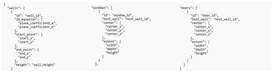
Figure 9. JSON file structure showing extracted features of walls, windows and doors.

3.3. Automated BIM Generation in Autodesk Revit

3.3.1. Geometric Data Import and Unit Conversion

The final stage of the workflow involves the automated generation of a BIM model within Autodesk Revit using RevitPythonShell 2023 and the Revit API. The JSON file containing geometric data is first imported, and all coordinates and dimensions are converted from meters to feet using a conversion factor of 3.28084.

Before wall creation, a duplicate removal algorithm is applied to the JSON wall entries to eliminate repeated geometries. This is performed using a custom distance-based filter with a 0.1 m tolerance and an angular similarity threshold of 5 degrees. The filtering process removes geometrically redundant wall entries, such as identical or reversed start and end points, to make sure walls representing the same physical structure are not created multiple times due to minor geometric variation or noise. This leads to a clean and minimal wall layout suitable for BIM integration.

3.3.2. Wall Creation, Door and Window Placement, and Host Assignment

Walls are created by constructing line elements between the start and end coordinates obtained from the JSON file and assigning the corresponding wall heights. A predefined wall type is selected from the available project elements, and each wall is instantiated using the Wall. Create a method by passing a Line object defined between the start and end points. This is performed within a Revit transaction. The created wall elements are indexed using their custom IDs to allow subsequent steps such as window and door placement, to correctly reference and attach elements to the appropriate host walls.

Following the generation of wall geometry, door and window family instances are created. For each door and window, an insertion point is calculated directly from the center coordinates provided in the JSON file. The host wall is determined by matching the custom wall identifier. However, if a direct match fails due to duplicate removal, a fallback mechanism is employed. This mechanism computes the minimum distance between the element’s insertion point and all wall segments using 2D point-to-line proximity. The nearest wall is then assigned as the host to make sure that every door and window is correctly embedded within a wall geometry.

A door family symbol is then retrieved and activated from the project, and a new door instance is placed at the computed insertion point. Similarly, for each window, the corresponding family symbol is retrieved and activated before instantiation at the specified coordinates. All modifications are performed within the same Revit transaction, and upon completion, the transaction is committed to finalizing the BIM model. Algorithm 3 illustrates the BIM modeling in Revit workflow using RevitPythonShell in pseudocode. Figure 10 shows the BIM model generated from the JSON file.

Algorithm 3: Automated BIM Generation in Autodesk Revit

Input: BIM data in JSON format: ${\mathit{D}}_{\mathit{B}\mathit{I}\mathit{M}}$ Revit wall type, window type, and door type: ${\mathit{T}}_{\mathit{w}\mathit{a}\mathit{l}\mathit{l}}$, ${\mathit{T}}_{\mathit{w}\mathit{i}\mathit{n}}$, ${\mathit{T}}_{\mathit{d}\mathit{o}\mathit{o}\mathit{r}}$ Tolerance for duplicate walls: ${\mathit{\tau }}_{\mathit{d}\mathit{u}\mathit{p}}$ Angular similarity threshold: ${\mathit{\phi }}_{\mathit{s}\mathit{i}\mathit{m}}$ Conversion factor: meters_to_feet Output: Walls, doors, and windows placed in the Revit project.

Initialize: ○ Load ${\mathit{D}}_{\mathit{B}\mathit{I}\mathit{M}}$ from the JSON file. ○ Convert all dimensions from meters to feet using meters_to_feet. Define function RemoveDuplicateWalls(${\mathit{D}}_{\mathit{B}\mathit{I}\mathit{M}},{\mathit{\tau }}_{\mathit{d}\mathit{u}\mathit{p}}$, ${\mathit{\phi }}_{\mathit{s}\mathit{i}\mathit{m}}$): ○ For each pair of walls in ${\mathit{D}}_{\mathit{B}\mathit{I}\mathit{M}}$ ▪ Compare start and end points of both walls. ▪ Compute direction vectors of the wall segments. ○ If the distance between endpoints < ${\mathit{\tau }}_{\mathit{d}\mathit{u}\mathit{p}}$ and angular difference between direction vectors < ${\mathit{\phi }}_{\mathit{s}\mathit{i}\mathit{m}}$. ▪ Mark one wall as duplicate. ○ Remove marked duplicates from ${\mathit{D}}_{\mathit{B}\mathit{I}\mathit{M}}$. ○ Return: Filtered wall data. End function Call RemoveDuplicateWalls(${\mathit{D}}_{\mathit{B}\mathit{I}\mathit{M}},{\mathit{\tau }}_{\mathit{d}\mathit{u}\mathit{p}}$, ${\mathit{\phi }}_{\mathit{s}\mathit{i}\mathit{m}}$) Start a transaction in Revit. Define function CreateWalls(${\mathit{D}}_{\mathit{B}\mathit{I}\mathit{M}},{\mathit{T}}_{\mathit{w}\mathit{a}\mathit{l}\mathit{l}}$): ○ Find ${\mathit{T}}_{\mathit{w}\mathit{a}\mathit{l}\mathit{l}}$ in the Revit project. ○ Get the level in the project. ○ For each wall in ${\mathit{D}}_{\mathit{B}\mathit{I}\mathit{M}}$: ▪ Extract start point, end point, and height. ▪ Create a wall using Revit API and Store the created wall. ○ Return: Created walls and their heights. End function Call CreateWalls(${\mathit{D}}_{\mathit{B}\mathit{I}\mathit{M}},{\mathit{T}}_{\mathit{w}\mathit{a}\mathit{l}\mathit{l}}$) to create walls. Define function CreateDoors(${\mathit{D}}_{\mathit{B}\mathit{I}\mathit{M}}, walls, {\mathit{T}}_{\mathit{d}\mathit{o}\mathit{o}\mathit{r}}$): ○ For each door in ${\mathit{D}}_{\mathit{B}\mathit{I}\mathit{M}}$: ▪ Find ${\mathit{T}}_{\mathit{d}\mathit{o}\mathit{o}\mathit{r}}$ in the Revit project. ▪ Find the host wall using the wall ID or the duplicate mapping if necessary. ▪ Place door in Revit at the specified insertion point. End function Call CreateDoors(${\mathit{D}}_{\mathit{B}\mathit{I}\mathit{M}}, walls, {\mathit{T}}_{\mathit{d}\mathit{o}\mathit{o}\mathit{r}}$). Define function CreateWindows(${\mathit{D}}_{\mathit{B}\mathit{I}\mathit{M}}, walls, {\mathit{T}}_{\mathit{w}\mathit{i}\mathit{n}}$): ○ For each window in ${\mathit{D}}_{\mathit{B}\mathit{I}\mathit{M}}$: ▪ Find ${\mathit{T}}_{\mathit{w}\mathit{i}\mathit{n}}$ in the Revit project. ▪ Find the host wall using the wall ID or the duplicate mapping if necessary. ▪ Place window in Revit at the specified insertion point. End function Call CreateWindows(${\mathit{D}}_{\mathit{B}\mathit{I}\mathit{M}}, walls, {\mathit{T}}_{\mathit{w}\mathit{i}\mathit{n}}$). Commit the transaction. Return: Successfully created walls, doors, and windows in Revit.

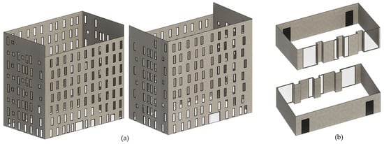
Figure 10. Automated BIM models generated from JSON data in Revit using RevitPythonShell for (a) Dataset 1 and (b) Dataset 2.

3.4. Evaluation Metrics

This section presents the evaluation framework used to assess the effectiveness of the proposed image-to-BIM method. The assessment is organized into two parts: (1) benchmarking the performance of the three NeRF models utilized in the reconstruction stage, and (2) evaluating the semantic, spatial, and geometric quality of the final generated BIM.

3.4.1. NeRF Model Performance Analysis

To comprehensively assess the suitability of each NeRF model for integration into the automated image-to-BIM workflow, a multi-criteria evaluation was conducted to examine critical aspects of model performance, including pose estimation accuracy, computational efficiency, training time, reconstruction and rendering quality, and the practical PC quality for geometry extraction.

Camera Pose Recovery Analysis examined the relationship between dataset size and successful camera pose estimation. COLMAP, integrated within the Nerfstudio framework, was used to evaluate the percentage of recovered poses across varying input sizes. This analysis is important, as the accuracy of pose estimation directly affects the completeness and reliability of NeRF-based 3D reconstruction. Controlled experiments were conducted using image subsets ranging from 50 to 550 frames to determine the minimum data volume required for stable and accurate pose registration.

Computational Resource Efficiency was evaluated by monitoring system resource usage, including Central Processing Unit (CPU), Graphics Processing Unit (GPU), and Random Access Memory (RAM) consumption, throughout the training process for each NeRF model. All measurements were recorded under consistent experimental conditions. A high-performance system equipped with an Intel Core Ultra 9 185H CPU and an NVIDIA RTX 4090 GPU was used to ensure a fair comparison and to eliminate hardware-related bottlenecks.

Training Time Analysis was conducted to evaluate the training efficiency of each NeRF model under varying data conditions. Each model was benchmarked using datasets containing 150 to 550 input frames to assess how both the volume of input data and the underlying model architecture influence total training time.

Reconstruction Quality and Rendering Performance were evaluated across the NeRF models using multiple standard metrics applied to datasets of increasing input size. Peak Signal-to-Noise Ratio (PSNR) was used to quantify image reconstruction fidelity, where higher values indicate better visual accuracy. SSI measured the preservation of structural details in the reconstructed scene. Learned Perceptual Image Patch Similarity (LPIPS), which captures perceptual differences between images based on deep feature representations, was also analyzed, with lower values reflecting better perceptual similarity. In addition to visual quality, rendering performance was assessed by calculating the average number of Rays Processed Per Second (RPS), which reflects computational throughput, and the average number of Frames Per Second (FPS), which indicates overall rendering speed.

PC Quality for Geometry Extraction was analyzed to determine each NeRF model’s effectiveness in producing structured and usable spatial data for downstream processing. In this workflow, the PC reconstructed by each NeRF model serves as the input for geometric reasoning tasks, including element detection and spatial representation of architectural components. The process incorporates color-coded segmentation, plane fitting, clustering, and axis-aligned geometry extraction to identify walls, windows, and doors. Consequently, the spatial accuracy, structural clarity, and noise level of the generated PCs directly influence the automatic geometry extraction. Models that generate clean, high-fidelity PCs result in more accurate segmentation, fewer false positives, and better alignment of extracted geometry within the final BIM model.

3.4.2. Automated BIM Creation Performance Evaluation

This subsection outlines the quantitative criteria used to evaluate the performance of the proposed image-to-BIM method in generating semantically accurate and geometrically reliable BIM models. The evaluation focuses on three critical dimensions: semantic accuracy, spatial fidelity, and geometric precision of the generated BIM elements.

Semantic Accuracy was assessed by comparing the automatically detected windows and doors in the final BIM output against ground-truth annotations. This criterion evaluates the method’s ability to accurately identify and classify building elements within the reconstructed scene. Spatial Fidelity was measured through area-based overlap analysis between the predicted and ground-truth footprints. Metrics such as precision, recall, F1 score, and IoU were used to quantify the degree of alignment between predicted and actual spatial layouts. Geometric Precision focused on the dimensional consistency of extracted elements. Specifically, the perimeter measurements of detected objects were compared against ground-truth references to assess scale accuracy and geometric conformity.

To evaluate the spatial accuracy of the extracted building elements, this study employed widely adopted metrics including Precision (Correctness), Recall (Completeness), F1 Score, and IoU. Precision is defined as the ratio of the intersection area to the predicted area, while Recall measures the ratio of the intersection area to the actual area. The F1 Score, as the harmonic mean of Precision and Recall, provides a balanced indication of model performance. These metrics are commonly used in BIM evaluation benchmarks, as shown by Khoshelham et al. [59]. IoU, defined as the intersection area divided by the union of predicted and actual areas, is widely used in segmentation evaluations, as described by Yang et al. [50].

The specific formulas used to compute these spatial metrics are as follows:

• Intersection Area: Region shared between predicted and actual areas.
• Precision (Correctness): Intersection Area/Predicted Area
• Recall (Completeness): Intersection Area/Actual Area
• F1 Score: 2 × (Precision × Recall)/(Precision + Recall)
• IoU: Intersection Area/(Actual Area + Predicted Area—Intersection Area)

This evaluation supports assessment of the method’s ability to convert 2D imagery into accurate, semantically rich, and geometrically aligned BIM models.

4. Results

This section presents the simulation results of the proposed image-to-BIM method, and covers both the performance of the NeRF models and the accuracy of BIM generation. Subsections highlight key findings on camera pose recovery, computational efficiency, training time, and rendering performance. The final stages focus on PC quality for geometry extraction and the precision of the generated BIM models. Results are structured to reflect technical performance and practical utility across interior and exterior datasets.

4.1. Camera Pose Recovery Analysis

The impact of image data size on camera pose estimation was examined to determine the minimum data volume required for stable NeRF initialization. As shown in Figure 11, the percentage of successfully recovered poses increases significantly with an increasing number of input frames. With 50 frames, COLMAP recovered just 4% of camera poses. The recovery rate gradually improves, reaching 36% at 100 frames and 55.5% at 200. A sharp increase occurs between 200 and 250 frames, where pose recovery exceeds 92%. Beyond this point, the performance plateaus, with recovery stabilizing between 94% and 98% from 250 to 550 frames. Notably, Nerfstudio’s default setting for frame extraction from video datasets is approximately 300 frames, which, based on these results, offers sufficiently high pose coverage for reliable NeRF reconstruction in many cases. In this study, 550 frames were used to ensure near-complete pose recovery for the exterior scene and to support the generation of dense and accurate 3D models.

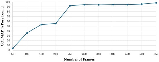
Figure 11. The relationship between the number of input frames and the percentage of successfully recovered poses using COLMAP in Nerfstudio.

This trend emphasizes the importance of spatial image overlap in achieving robust matching features. Visual gaps between consecutive views at lower frame counts limit COLMAP’s ability to identify consistent key points and reduce pose estimation success. As the number of frames increases, the likelihood of overlapping content improves. The observed jump in performance beyond 250 frames suggests that spatial coverage became sufficient for this particular case. However, the optimal threshold may vary depending on scene complexity, camera motion, and lighting conditions.

4.2. Computational Resource Efficiency

System resource usage was analyzed to compare the computational demands of the evaluated NeRF models during training. Figure 12 shows that CPU usage was highest for Nerfacto, which utilized an average of 52.9% of the CPU. Instant-NGP showed moderate usage at 31.4%, while Splatfacto maintained the lowest CPU load with an average of 5.3%. This highlights that Nerfacto’s volumetric pipeline and scene encoding require more CPU resources, whereas Splatfacto, driven primarily by GPU-based rasterization, places minimal demand on the CPU.

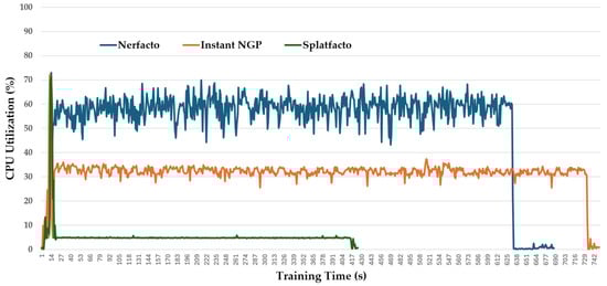
Figure 12. CPU usage percentage over training time across NeRF models.

GPU utilization patterns, shown in Figure 13, paint a different picture. Splatfacto demonstrated the highest average GPU usage at 81.7%, maintaining a high level of utilization throughout training. Instant-NGP followed with 66.9%, while Nerfacto averaged 45.8%. These values reflect the models’ varying reliance on GPU-intensive operations, with Splatfacto showing strong dependence on GPU rendering via Gaussian Splatting.

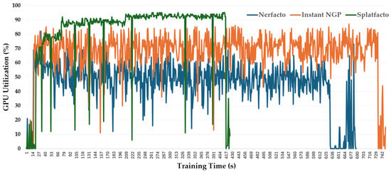
Figure 13. GPU usage percentage over training time across NeRF models.

Figure 14 combines both RAM and GPU memory usage across the training period. GPU memory consumption was lowest for Splatfacto, averaging 2.5 GB, followed by Instant-NGP at 3.3 GB and Nerfacto at 5.6 GB. In terms of RAM usage, Splatfacto again showed the smallest footprint with an average of 3.7 GB. Instant-NGP used approximately 6.7 GB, while Nerfacto maintained the highest RAM usage at around 11 GB throughout the training process. These observations highlight Splatfacto’s system and GPU memory efficiency, making it well-suited for resource-constrained environments.

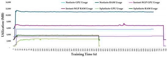
Figure 14. RAM and GPU memory usage over training time across NeRF models.

The results show that Splatfacto is the most efficient model, consistently combining high GPU utilization with the lowest CPU, system RAM, and GPU memory demands. Its high GPU load reflects efficient exploitation of modern hardware optimized for parallel processing and real-time rendering. This efficiency stems from its GPU-based Gaussian splatting approach, which offloads the bulk of computation to the GPU and minimizes CPU and memory overhead. In contrast, Nerfacto delivers high-quality volumetric reconstructions but places the most significant strain on CPU and system memory, consistent with the complexity of its architecture. Instant-NGP offers a balanced profile, achieving faster training with moderate usage of all system resources. These findings inform the selection of a NeRF model, considering hardware availability, training efficiency, and application-specific objectives. A deeper exploration of how these computational trade-offs relate to reconstruction accuracy and practical deployment is presented in Section 4.4.

4.3. Training Time Analysis

Training duration was benchmarked across NeRF models to assess time efficiency under consistent hardware and data conditions. As illustrated in Figure 15, Splatfacto consistently achieved the fastest training times across all tested configurations. Its training duration ranged from 410 to 439 s, averaging 425.8 s overall. This performance is directly attributed to its reliance on GPU-accelerated Gaussian splatting, which optimizes the rendering process. In contrast, Nerfacto required longer to complete training, with times ranging from 682 to 694 s and an average of 688.8 s. The higher training time reflects the complexity of Nerfacto’s volumetric rendering pipeline and its greater reliance on CPU and memory resources, as previously discussed in Section 4.2. Instant-NGP, while recognized for its fast convergence and efficiency in NeRF literature, showed the longest training times in this evaluation. With durations ranging from 736 to 762 s and an average of 749.4 s, it lagged behind Splatfacto and Nerfacto under identical hardware.

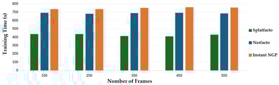
Figure 15. Training time comparison across evaluated NeRF models.

Overall, the comparison highlights Splatfacto as the most time-efficient model in this setup, offering rapid training regardless of input size. Interestingly, the number of input frames had a minimal impact on the overall training time for any evaluated models. Each model maintained a consistent training duration despite varying the dataset size.

4.4. Reconstruction Quality and Rendering Performance

Reconstruction fidelity and rendering speed were evaluated to compare the visual quality and throughput efficiency of the NeRF models. As shown in Figure 16, Splatfacto consistently achieves the highest PSNR values across all frame counts, ranging from 17.79 at 150 to 22.88 at 550 frames. Instant-NGP follows with values between 17.16 and 18.95, while Nerfacto performs the weakest, improving gradually from 15.63 to 18.52. This indicates that Splatfacto produces sharper and less noisy reconstructions, especially as scene coverage increases.

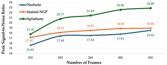
Figure 16. PNSR comparison across evaluated NeRF models.

Similarly, Figure 17 shows that Splatfacto leads in SSI, progressing from 0.69 to 0.86 as the number of frames increases. Instant-NGP improves steadily from 0.65 to 0.73, while Nerfacto again lags behind, rising from 0.62 to 0.68. Results highlight Splatfacto’s stronger ability to preserve structural fidelity and perceptual quality in the rendered outputs.

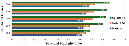
Figure 17. SSI comparison across evaluated NeRF models.

The LPIPS evaluation, presented in Figure 18, shows that Splatfacto achieves the lowest perceptual error across all input sizes. As frames increase from 150 to 550, LPIPS values for Splatfacto consistently decrease from 0.31 to 0.15, reflecting a closer perceptual match between the reconstructed and reference images. Instant-NGP shows moderate performance, with values decreasing from 0.44 to 0.34. Nerfacto shows relatively higher LPIPS values, starting at 0.47 and decreasing to 0.35 as the number of frames increases, ultimately approaching the performance of Instant-NGP at higher input sizes. These results indicate that Splatfacto produces more visually faithful reconstructions, especially in scenarios with richer input data.

Figure 18. LPIPS comparison across evaluated NeRF models.

Beyond visual quality, rendering performance results in Table 1 show a clear computational advantage for Splatfacto. It processes approximately 71,295,630 rays per second and generates 137.924 frames per second, significantly outperforming Nerfacto, which reaches 838,423 rays and 1.616 frames per second, and Instant-NGP, which handles 341,203 rays and 0.654 frames per second. This high efficiency comes from Splatfacto’s Gaussian splatting architecture that avoids volumetric sampling and neural field queries, allowing much faster rendering.

Table 1. Rendering speed comparison of NeRF models based on rays and frames per second.

Metrics	Instant NGP	Nerfacto	Splatfacto
Num Rays Per Sec	341,203	838,423	71,295,630
Num Frames per Sec	0.654	1.616	137.924

The results highlight the trade-offs among the evaluated models. Splatfacto delivers the highest reconstruction quality and rendering speed, making it a strong choice for scenarios that prioritize both fidelity and efficiency. Nerfacto produces reasonably good visual quality but requires more CPU and memory resources and renders more slowly due to its volumetric processing pipeline. Instant-NGP shows moderate visual quality and computational demand performance, but it falls short of Splatfacto in rendering speed and output precision.

4.5. Practical PC Quality for Geometry Extraction

To evaluate each model’s suitability for geometric feature extraction, the structural clarity and consistency of the reconstructed PC were analyzed. Figure 19 presents the extracted PCs from the reconstructed interior scene using each NeRF model, illustrating both front and rear views of the classroom. These color-labeled outputs visually demonstrate each reconstruction’s structural completeness and spatial clarity. Among the three models, the PC generated by Nerfacto exhibits the most consistent geometry and clean surface representation. Wall boundaries, furniture contours, and door/window regions appear sharp and continuous, providing a stable foundation for geometric segmentation and facilitating accurate alignment in downstream processing. The Instant-NGP output retains recognizable scene layout but introduces soft edges and localized noise, particularly near object boundaries. While core architectural features remain identifiable, the reduced edge sharpness may introduce spatial ambiguity during plane fitting or clustering, affecting the precision of wall, window, and door extraction.

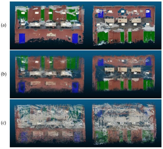
Figure 19. Generated color-labeled point clouds showing front and back of the classroom (Dataset 2) extracted from (a) Nerfacto, (b) Instant NGP, and (c) Splatfacto model.

Although Splatfacto excels in reconstruction quality, training speed, and rendering efficiency, its integration into geometry extraction workflows presents practical limitations. Since Splatfacto reconstructs scenes using 3D Gaussian splats and lacks native PC export in Nerfstudio, this study employed the 3DGS-to-PC framework by Stuart and Pound [60] to convert splats into PCs. This framework samples points from Gaussians based on their volume, filters outliers using Mahalanobis distance, and recalculates colors from rendered images to improve visual accuracy. However, the converted outputs are shown in Figure 19 contain structural noise, such as floating clusters, blurred edges, and irregular densities that obscure object boundaries and disrupt spatial consistency. Although Splatfacto achieves high PSNR and SSI scores, these irregularities in the PCs hinder accurate wall, window, and door classification and extraction within the Image to BIM workflow.

4.6. Automated BIM Creation Results and Evaluation

The final phase of the proposed method was assessed through the generation of BIM models from reconstructed scenes. This subsection presents the results on semantic accuracy, spatial alignment, and geometric precision, based on comparisons between the generated output and ground-truth annotations. As shown in Figure 6, the reconstruction process using segmented images enables precise label transfer and results in a successful reconstructed 3D scene where building elements such as walls, windows, and doors are preserved across the scene with their predefined colors. Building on this labeled reconstruction, Figure 7 displays the exported color-labeled PCs, which serve as the input for subsequent processing. Geometric features are then extracted through wall plane fitting and object clustering, as illustrated in Figure 8. These extracted elements are automatically serialized and imported into Autodesk Revit to generate the final BIM model, shown in Figure 10. Together, these stages demonstrate the method’s ability to maintain semantic integrity, capture accurate geometry, and produce a structured and automation-ready BIM output directly from 2D imagery.

The workflow’s performance is evaluated using three critical criteria: (1) semantic accuracy in detecting windows and doors, (2) geometric precision evaluated using perimeter comparisons, and (3) spatial fidelity assessed through area-based overlap metrics.

Table 2 presents the number of doors and windows in the analysis of the semantic feature extraction results in both datasets. The proposed method correctly identified all architectural elements: 248 windows and four doors in Dataset 1, and 4 windows and two doors in Dataset 2. This perfect match with the ground truth highlights the reliability of the element detection process and confirms the method’s ability to maintain semantic precision across different scene types.

Table 2. Doors and windows identified in the datasets using the proposed method.

Building Dataset	No. of Actual Windows	No. of Predicted Windows	No. of Actual Doors	No. of Predicted Doors	Window Accuracy	Door Accuracy
Dataset 1	248	248	4	4	100%	100%
Dataset 2	4	4	2	2	100%	100%

To contextualize these results, Table 3 compares door and window extraction performance against previous Scan-to-BIM studies that employed PC-based and image-based approaches. Across references [22,46,61,62], reported accuracies for door and window instance detection range between 96 and 100 percent. Due to various types and meanings for accuracy, the clarification is needed that the successful identification of an element is assumed as accuracy in detection. The proposed image-to-BIM method achieves results consistent with these benchmarks, which match the highest reported accuracies in detecting an element without reliance on laser scanning or PC input. In these benchmark studies, the number of detected windows and doors ranged from 0 to 28, whereas the proposed method successfully detected up to 248 windows without any error.

Table 3. Selected studies comparing the accuracy of successfully detecting doors and windows in their chosen case studies.

Method/Dataset	No. of Actual Windows	No. of Predicted Windows	No. of Actual Doors	No. of Predicted Doors	Window Accuracy	Door Accuracy
[46]/Collected 1,2	21	21	25	24	100%	96%
[61]/Dataset 1, 2, 3	7	7	6	6	100%	100%
[62]/Data 1,2	4	4	4	4	100%	100%
[22]/Average	28	28	11	11	100%	100%

Further geometric evaluation was conducted using perimeter accuracy. As shown in Table 4. The proposed method demonstrated a strong ability to maintain geometric consistency between the reconstructed models and ground-truth buildings. For Dataset 1, the predicted perimeter was 100.38 m, compared to the actual perimeter of 100.32 m, resulting in a minimal deviation of 0.06 m and an accuracy of 99.94%. For Dataset 2, the predicted perimeter was 37.83 m versus an actual value of 37.27 m, with an error of 0.56 m and an accuracy of 98.49%.

Table 4. Evaluation of the reconstructed BIM model based on predicted perimeters.

Building Dataset	Actual Perimeter (m)	Predicted Perimeter (m)	Error (m)	Accuracy (%)
Dataset 1	100.32	100.38	0.06	99.94
Dataset 2	37.27	37.83	0.56	98.49

Table 5 compares the proposed method’s perimeter accuracy with previously published results. In the benchmark study [46], perimeter deviations ranged from 0.019 to 0.929 m, corresponding to accuracies between 99.30 and 99.90 percent. The proposed image-to-BIM approach achieves comparable geometric precision.

Table 5. Quantitative comparison of reconstructed BIM model based on predicted perimeters.

Method/Dataset	Actual Perimeter (m)	Predicted Perimeter (m)	Error (m)	Accuracy (%)
[46]/Collected 1	149.734	150.663	−0.929	99.30
[46]/Collected 2	27.492	27.473	0.019	99.90

Table 6 presents the spatial accuracy evaluation based on area comparisons. For Dataset 1, the predicted building footprint aligns closely with the reference geometry, achieving a precision of 0.994, a recall of 0.997, an F1 score of 0.996, and an IoU of 0.992. Dataset 2 reconstruction yields a predicted area of 83.06 m² and an intersection of 80.88 m², resulting in a precision of 0.974, a recall of 0.995, an F1 score of 0.984, and an IoU of 0.969. These metrics confirm the pipeline’s ability to preserve spatial accuracy and generate BIM models that consistently reflect real-world dimensions.

Table 6. Evaluation of the reconstructed BIM model based on predicted area.

Building Dataset	Actual Area (m2)	Predicted Area (m2)	Intersection Area (m2)	Precision	Recall	F1 Score	IoU
Dataset 1	583.17	585.20	581.71	0.994	0.997	0.996	0.992
Dataset 2	81.26	83.06	80.88	0.974	0.995	0.984	0.969

4.7. Comparative Analysis with Scan-to-BIM Literature

To contextualize the performance of the proposed method, a comparative analysis was conducted against several recent AI enhanced Scan-to-BIM approaches, as summarized in Table 7. The comparison demonstrates that the proposed method achieves state-of-the-art performance on both Dataset 1 and Dataset 2. Across the selected benchmark studies, evaluated metric values fall within the range of 0.93–0.999, and the proposed method performs at a comparable or higher level of spatial accuracy than traditional Scan-to-BIM. The slightly higher accuracy observed on Dataset 1 can be attributed to the superior input quality provided by the UAV’s stabilized 4K camera and structured flight path.

Table 7. Comparative evaluation of recent BIM reconstruction techniques based on predicted area.

Method	Dataset	Precision	Recall	F1 Score	IoU
The present study, Dataset 1: DJI Mini 4 Pro drone for image acquisition YOLO and SAM2 for image detection and segmentation NeRF for 3D reconstruction and PC generation		0.994	0.997	0.996	0.992
The present study, Dataset 2: Standard smartphone camera for image acquisition YOLO and SAM2 for image detection and segmentation NeRF for 3D reconstruction and PC generation		0.974	0.995	0.984	0.969
Mahmoud, Zhao [61]: Leica RTC360 3D laser scanner for PC acquisition RandLA-Net for PC semantic segmentation		0.994	0.996	0.995	0.990
Mahmoud, Chen [63]: NavVis M6 mobile laser scanner for PC acquisition RandLA-Net for semantic segmentation		0.991	0.993	0.992	0.984
Mahmoud, Li [62]: Faro Focus 3D laser range scanner for PC acquisition RandLA-Net for semantic segmentation		0.989	0.990	0.989	0.978
Mahmoud, Chen [46]: NavVis M6 indoor mobile mapping 3D scanner RandLA-Net for semantic segmentation		0.999	0.997	0.998	0.998
Gao et al. [64]: Mobile Laser Scanning for PC acquisition Mask R-CNN for semantic segmentation		0.930	0.970	0.950	-

Unlike conventional Scan-to-BIM studies the present method provides a more efficient and less expensive solution. For example, the conventional approach relies on costly LiDAR or laser-scanning hardware as well as PC processing and CNN-based PC segmentation networks such as RandLA-Net or Mask R-CNN. However, the proposed method performed detection and segmentation directly on RGB imagery using open-source vision–language models (YOLO and SAM) combined with NeRF or Gaussian Splatting for 3D reconstruction which is cost-free and removes the need for PC segmentation.

4.8. Comparative Analysis with NeRF-Based Methods

Recent NeRF-based reconstruction studies have introduced varying levels of automation; however, their workflow remains distinct from the method presented in this study. NeRF-to-BIM [65] demonstrated an initial attempt to couple NeRF reconstruction with BIM creation, where Instant-NeRF produced PCs later segmented by PointNeXt to classify structural elements such as beams and columns. Although this work verified the potential of NeRF-generated data for BIM applications, it required intensive post-processing and manual refinement. Harbingers of NeRF-to-BIM [66] extended this to a three-stage process combining NeRF reconstruction, fine-tuned PointNeXt segmentation on synthetic BIM-derived datasets, and BIM generation; however, it still relied on labeled PCs and separate training steps. Similarly, Li et al. [67] applied Nerfacto to reconstruct building façades from UAV imagery, followed by PointNet++ segmentation of the NeRF-derived PCs. Montas-Laracuente et al. [68] adopted Gaussian Splatting to generate high-fidelity meshes for heritage documentation but without semantic or BIM automation. In contrast, the proposed method explicitly advances this line of research by bypassing PC post-processing, embedding semantic information directly at the image level before NeRF training. This early-stage semantic integration allows class labels to propagate throughout the 3D reconstruction, resulting in PCs that are already color-segmented and labeled during generation. Consequently, precise geometry extraction can be performed without additional segmentation or manual refinement, thereby achieving a higher degree of automation and practical efficiency than previous NeRF-based approaches.

4.9. Comparative Analysis of Evaluated NeRF Models

Since the proposed method relies on NeRF-based reconstruction, selecting an appropriate model is important. Table 8 presents a detailed comparison of three NeRF models, evaluating them across visual fidelity, computational performance, and PC suitability for BIM extraction. Among them, Splatfacto delivers the highest reconstruction quality and speed, far surpassing the performance of Instant-NGP and Nerfacto. Despite its speed and visual quality, Splatfacto has practical limitations for Scan-to-BIM workflows. It does not natively export PCs, requiring an external conversion step that introduces structural noise and blurs object boundaries. As a result, the generated PC lacks the consistency needed for object extraction.

Table 8. Comparative evaluation of examined NeRF models.

Metrics	Instant NGP	Nerfacto	Splatfacto
Average Training Time	749.4	688.8	425.8
PSNR	18.95	18.52	22.88
SSI	0.73	0.68	0.86
LPIPS	0.34	0.35	0.15
Average CPU Utilization (%)	31.4	52.9	5.3
Average GPU Utilization (%)	66.9	45.8	81.7
Average RAM Utilization (GB)	6.7	11	3.7
Average GPU Utilization (GB)	3.3	5.6	2.5
Num RPS	341,203	838,423	71,295,630
Num FPS	0.654	1.616	137.924
Native PC Generation	Yes	Yes	No
PC quality for Geometry Extraction	Medium	High	Low

In contrast, while Nerfacto’s visual metrics are slightly lower than those of Splatfacto, it produces the most structured and spatially coherent PC outputs, making it more suitable for geometry extraction. Instant-NGP, while known for its speed in NeRF literature, shows longer training times in this evaluation and delivers moderate reconstruction quality. Its PCs exhibit soft edges and localized noise, which may hinder precise segmentation and alignment in BIM generation tasks. Nonetheless, it offers a balanced computational profile, with moderate resource efficiency. Overall, these findings suggest that Nerfacto is the most suitable model for geometry-aware applications, such as Scan-to-BIM, where spatial consistency is crucial.

5. Discussion

5.1. Key Contributions and Implications

The primary contribution of this work lies in offering a method for automated BIM generation from images using accessible hardware and open-source tools. It bridges critical gaps in the Scan-to-BIM literature by (1) demonstrating that BIM models can be generated from image data alone, eliminating reliance on scanning equipment by producing PCs directly from RGB images using NeRF volumetric rendering. This is achieved by integrating object-level semantic segmentation with NeRF-based 3D reconstruction in a unified method, allowing the system to learn spatial structure directly from labeled RGB inputs rather than relying on traditional photogrammetry or LiDAR-based scans; (2) demonstrating, for the first time, how semantic identity can be embedded into NeRF-based volumetric reconstruction and subsequently extracted as structured geometric data for BIM modeling. This removes the need for post-reconstruction segmentation by embedding semantic labels at the pixel level during preprocessing using computer vision-language techniques. These labels are preserved throughout the rendering process, eliminating projection-based mapping that might lead to misalignment and inconsistency, and ensuring that each building element retains its identity from image input to final BIM output; and (3) developing the workflow from image acquisition to BIM output without requiring domain-specific training data. The extracted geometry is serialized in a structured JSON format and directly imported into Revit, enabling automation of BIM model creation based on the building elements embedded semantic and geometric attributes.

Additionally, this study performs a comparative evaluation of three reconstruction methods, namely Instant-NGP, Nerfacto, and Splatfacto, in the context of Scan-to-BIM automation. It establishes criteria for selecting suitable models based on PC quality, rendering efficiency, and spatial fidelity, identifying Nerfacto as the most effective for geometry extraction. This may advance the application of NeRF models using the criteria beyond view synthesis and introduces them as viable tools for geometry-aware BIM modeling.

In practical terms, the proposed method transforms how existing buildings are digitized by eliminating the need for terrestrial scanning devices, or the tedious manual on-site surveying. Tasks that were once labor-intensive, equipment-dependent, and costly such as site surveying and digital modeling, can benefit from using widely accessible camera devices, expanding the practicality and scalability of BIM-based planning across the construction and facilities sector.

The framework is especially impactful for aging, undocumented, or under-maintained buildings, where original drawings are often unavailable. It facilitates rapid creation of digital twins for a wide range of practical applications, including renovation planning, space optimization, and exterior façade restoration. The resulting BIM model is generated directly within Revit using native building elements, which enables compatibility with existing BIM workflows. It functions not only as a geometric record but also it can be useful as an operational asset for facility management tasks such as quantity take-offs, material tracking, and renovation cost estimation performed directly within the Revit environment. Furthermore, the model can be exported from Revit to open formats such as IFC, supporting interoperability with facility management and asset information systems commonly used in practice. In energy retrofit scenarios, the method provides reliable building geometry for tasks such as insulation upgrades, envelope improvements, and solar panel placement, where models can be used directly within Revit for energy analyses or exported to IDF or gbXML formats for integration with tools like EnergyPlus and OpenStudio. However, all these applications need to be tested and evaluated as future studies. The accessibility and speed of this approach could make it a compelling solution for practitioners seeking to modernize building data acquisition workflows without the burden of costly hardware or extensive manual effort.

5.2. Limitations and Future Research Direction

Despite its strengths, the study identified limitations as well. First, NeRF reconstruction quality remains sensitive to image completeness and clarity, and occlusions or inadequate image coverage can compromise model accuracy and completeness. Moreover, lighting variation, textureless or reflective surfaces, and the presence of dynamic objects during image capture may further reduce reconstruction fidelity by introducing inconsistencies in color, depth, and surface definition, which can ultimately lead to reconstruction failure. Second, the performance of the proposed Image-to-BIM workflow was validated on two scenes, one exterior and one interior, as a proof of concept. However, broader validation on buildings featuring intricate or unconventional architectural styles remains untested, which may affect its generalizability. Future research should extend the evaluation to a wider range of typologies, including heritage buildings and complex geometries, to assess the scalability and robustness of the method across diverse architectural conditions.

Third, the present system focuses exclusively on core building elements such as walls, doors, and windows. To enhance the versatility and completeness of this method, future investigations should expand semantic classification and geometric reconstruction capabilities to other building components, including floors, ceilings, columns, stairs, and complex internal spatial layouts. Fourth, While this study successfully automates several fragmented components of the image-to-BIM workflow, including segmentation, reconstruction, element extraction, and BIM creation, future work should focus on developing an end-to-end unified framework that seamlessly integrates all stages into a single automated pipeline. Fifth, while Gaussian splatting methods such as Splatfacto showed the highest potential in reconstruction quality, the lack of native PC export in current implementations remains a limitation. Future work should address this gap to unlock the full utility of Gaussian-based reconstructions in geometry-driven BIM applications. Sixth, incorporating adaptive parameter adjustments within geometric algorithms could improve performance and flexibility across architectural typologies and conditions.

Seventh, a comprehensive ablation study should be conducted to evaluate the contribution of each component, including YOLO for detection, SAM for segmentation, NeRF and Gaussian Splatting for reconstruction, and to optimize their interaction within the framework. This will clarify each module’s impact on accuracy and efficiency and guide future improvements in the image-to-BIM workflow. Eighth, all experiments were conducted on a high-end RTX 4090 GPU, which significantly reduced training time. Future research should evaluate the framework’s scalability on mid-range GPUs and cloud-based computing platforms to ensure broader accessibility and assess performance trade-offs under different hardware configurations. Lastly, while the proposed method effectively creates BIM models for undocumented buildings, future research should focus on extending the framework to enable continuous maintenance and digital twin updates by allowing new image inputs to be reprocessed to detect and integrate physical changes within the existing building model.

6. Conclusions

This study introduced an automated image-to-BIM method that integrates vision-language segmentation, NeRF-based 3D reconstruction, and structured geometric modeling to generate semantically rich and spatially accurate BIM models from ordinary 2D images. Experimental validation demonstrates that the proposed method achieves strong semantic, spatial, and geometric performance while eliminating the need for traditional scanning tools such as LiDAR or photogrammetry. Its key novelty lies in unifying semantic segmentation and 3D reconstruction in the chosen context, by embedding object labels during NeRF processing, thereby removing the need for post-processing on PCs and enabling a more efficient method to automatically generate BIM model.

Experimental validation confirms the method’s high performance across both semantic and geometric dimensions considering its limitations. The system successfully detected windows and doors across two distinct datasets: an exterior scene captured via UAV and an interior scene recorded with a handheld smartphone. In area-based evaluations, the method achieved a precision of 0.994, an IoU of 0.992 for the exterior case, and 0.974 precision with 0.969 IoU for the interior case. Perimeter comparisons confirmed geometric consistency, with deviations of just 0.06 m and 0.56 m for the exterior and interior datasets, yielding accuracies of 99.94% and 98.49%, respectively. The proposed method consistently achieved superior performance in comparative evaluations against recent deep learning-based reconstruction methods. It recorded higher precision (up to 0.994), F1 scores (up to 0.996), and IoU values (up to 0.992), outperforming existing approaches.

In evaluating three NeRF variants, Splatfacto demonstrated the highest image-based reconstruction quality, with PSNR of 22.88, SSI of 0.86, and LPIPS of 0.15, alongside industry-leading rendering speeds of 137.9 FPS and 71M rays per second. However, due to structural artifacts and density inconsistencies introduced during PC conversion, Splatfacto proved less effective for downstream geometric extraction. In contrast, Nerfacto, while slightly lower in visual quality, generated cleaner, more structured PCs that enabled more reliable element detection, making it a more suitable choice for geometry-aware BIM modeling within the proposed method.

By removing reliance on expensive scanning hardware and minimizing technical barriers, this method presents a scalable and accessible alternative for automated BIM generation. Its applicability spans a wide range of real-world use cases, including architectural documentation, renovation planning, energy retrofitting, facility management, and digital twin development. This work not only demonstrates a practical, low-cost pathway for digitizing existing buildings but also contributes to the theoretical advancement of image-driven reconstruction by establishing a new benchmark for semantic-aware NeRF-based Scan-to-BIM automation.

References

- Kaashi, S.; Vilventhan, A. Development of a building information modelling based decision-making framework for green retrofitting of existing buildings. J. Build. Eng. 2023, 80, 108128. [Google Scholar] [CrossRef]
- Wang, D.; Jiang, Q.; Liu, J. Deep-Learning-Based Automated Building Information Modeling Reconstruction Using Orthophotos with Digital Surface Models. Buildings 2024, 14, 808. [Google Scholar] [CrossRef]
- Mehraban, M.H.; Alnaser, A.A.; Sepasgozar, S.M.E. Building Information Modeling and AI Algorithms for Optimizing Energy Performance in Hot Climates: A Comparative Study of Riyadh and Dubai. Buildings 2024, 14, 2748. [Google Scholar] [CrossRef]
- Mehraban, M.H.; Sepasgozar, S.M.; Ghomimoghadam, A.; Zafari, B. AI-Enhanced Automation of Building Energy Optimization Using a Hybrid Stacked Model and Genetic Algorithms: Experiments with Seven Machine Learning Techniques and a Deep Neural Network. Results Eng. 2025, 26, 104994. [Google Scholar] [CrossRef]
- Mehraban, M.H.; Mirzabeigi, S.; Faraji, S.; Soltanian-Zadeh, S.; Sepasgozar, S.M.E. AI-Driven Prediction of Building Energy Performance and Thermal Resilience During Power Outages: A BIM-Simulation Machine Learning Workflow. Buildings 2025, 15, 3950. [Google Scholar] [CrossRef]
- Rocha, G.; Mateus, L.; Fernández, J.; Ferreira, V. A Scan-to-BIM Methodology Applied to Heritage Buildings. Heritage 2020, 3, 47–67. [Google Scholar] [CrossRef]
- Badenko, V.; Fedotov, A.; Zotov, D.; Lytkin, S.; Volgin, D.; Garg, R.; Liu, M. Scan-to-Bim Methodology Adapted for Different Application. ISPRS Int. Arch. Photogramm. Remote Sens. Spat. Inf. Sci. 2019, 42, 1–7. [Google Scholar] [CrossRef]
- Jung, J.; Hong, S.; Jeong, S.; Kim, S.; Cho, H.; Hong, S.; Heo, J. Productive modeling for development of as-built BIM of existing indoor structures. Autom. Constr. 2014, 42, 68–77. [Google Scholar] [CrossRef]
- Hong, S.; Jung, J.; Kim, S.; Cho, H.; Lee, J.; Heo, J. Semi-automated approach to indoor mapping for 3D as-built building information modeling. Comput. Environ. Urban Syst. 2015, 51, 34–46. [Google Scholar] [CrossRef]
- Volk, R.; Stengel, J.; Schultmann, F. Building Information Modeling (BIM) for existing buildings—Literature review and future needs. Autom. Constr. 2014, 38, 109–127. [Google Scholar] [CrossRef]
- Macher, H.; Landes, T.; Grussenmeyer, P. From Point Clouds to Building Information Models: 3D Semi-Automatic Reconstruction of Indoors of Existing Buildings. Appl. Sci. 2017, 7, 1030. [Google Scholar] [CrossRef]
- Cotella, V.A. From 3D point clouds to HBIM: Application of Artificial Intelligence in Cultural Heritage. Autom. Constr. 2023, 152, 104936. [Google Scholar] [CrossRef]
- Hübner, P.; Weinmann, M.; Wursthorn, S.; Hinz, S. Automatic voxel-based 3D indoor reconstruction and room partitioning from triangle meshes. ISPRS J. Photogramm. Remote Sens. 2021, 181, 254–278. [Google Scholar] [CrossRef]
- Bello, S.A.; Yu, S.; Wang, C.; Adam, J.M.; Li, J. Review: Deep Learning on 3D Point Clouds. Remote Sens. 2020, 12, 1729. [Google Scholar] [CrossRef]
- Tran, H.; Khoshelham, K. Procedural Reconstruction of 3D Indoor Models from Lidar Data Using Reversible Jump Markov Chain Monte Carlo. Remote Sens. 2020, 12, 838. [Google Scholar] [CrossRef]
- Borkowski, A.S.; Kubrat, A. Integration of Laser Scanning, Digital Photogrammetry and BIM Technology: A Review and Case Studies. Eng 2024, 5, 2395–2409. [Google Scholar] [CrossRef]
- Lichti, D.; Gordon, S.; Stewart, M.; Franke, J.; Tsakiri, M. Comparison of Digital Photogrammetry and Laser Scanning. In Proceedings of the ISPRS Commission II Symposium 2002: Integrated System for Spatial Data Production, Custodian and Decision Support, Xi’an, China, 20–23 August 2002. [Google Scholar]
- Rashdi, R.; Martínez-Sánchez, J.; Arias, P.; Qiu, Z. Scanning Technologies to Building Information Modelling: A Review. Infrastructures 2022, 7, 49. [Google Scholar] [CrossRef]
- Lato, M.; Kemeny, J.; Harrap, R.M.; Bevan, G. Rock bench: Establishing a common repository and standards for assessing rockmass characteristics using LiDAR and photogrammetry. Comput. Geosci. 2013, 50, 106–114. [Google Scholar] [CrossRef]
- Pantoja-Rosero, B.G.; Achanta, R.; Kozinski, M.; Fua, P.; Perez-Cruz, F.; Beyer, K. Generating LOD3 building models from structure-from-motion and semantic segmentation. Autom. Constr. 2022, 141, 104430. [Google Scholar] [CrossRef]
- Kim, H.; Remaggi, L.; Jackson, P.J.; Fazi, F.M.; Hilton, A. 3D Room Geometry Reconstruction Using Audio-Visual Sensors. In Proceedings of the 2017 International Conference on 3D Vision (3DV), Qingdao, China, 10–12 October 2017; pp. 621–629. [Google Scholar]
- Wong, M.O.; Sun, Y.; Ying, H.; Yin, M.; Zhou, H.; Brilakis, I.; Kelly, T.; Lam, C.C. Image-based scan-to-BIM for interior building component reconstruction. Autom. Constr. 2025, 173, 106091. [Google Scholar] [CrossRef]
- Armeni, I.; Sener, O.; Zamir, A.R.; Jiang, H.; Brilakis, I.; Fischer, M.; Savarese, S. 3D Semantic Parsing of Large-Scale Indoor Spaces. In Proceedings of the 2016 IEEE Conference on Computer Vision and Pattern Recognition (CVPR), Las Vegas, NA, USA, 27–30 June 2016; pp. 1534–1543. [Google Scholar]
- Cai, G.; Pan, Y. Understanding the Imperfection of 3D point Cloud and Semantic Segmentation algorithms for 3D Models of Indoor Environment. AGILE GISci. Ser. 2022, 3, 2. [Google Scholar] [CrossRef]
- Zhou, B.; Zhao, H.; Puig, X.; Fidler, S.; Barriuso, A.; Torralba, A. Scene Parsing through ADE20K Dataset. In Proceedings of the 2017 IEEE Conference on Computer Vision and Pattern Recognition (CVPR), Honolulu, HI, USA, 21–26 July 2017; pp. 5122–5130. [Google Scholar]
- Silberman, N.; Hoiem, D.; Kohli, P.; Fergus, R. Indoor Segmentation and Support Inference from RGBD Images. In Proceedings of the Computer Vision—ECCV 2012, Berlin/Heidelberg, Germany, 7–13 October 2012; pp. 746–760. [Google Scholar]
- Wong, M.O.; Ying, H.; Yin, M.; Yi, X.; Xiao, L.; Duan, W.; He, C.; Tang, L. Semantic 3D reconstruction-oriented image dataset for building component segmentation. Autom. Constr. 2024, 165, 105558. [Google Scholar] [CrossRef]
- Tang, P.; Huber, D.; Akinci, B.; Lipman, R.; Lytle, A. Automatic reconstruction of as-built building information models from laser-scanned point clouds: A review of related techniques. Autom. Constr. 2010, 19, 829–843. [Google Scholar] [CrossRef]
- Xiong, X.; Adan, A.; Akinci, B.; Huber, D. Automatic creation of semantically rich 3D building models from laser scanner data. Autom. Constr. 2013, 31, 325–337. [Google Scholar] [CrossRef]
- Croce, V.; Bevilacqua, M.G.; Caroti, G.; Piemonte, A. Connecting Geometry and Semantics Via Artificial Intelligence: From 3D Classification of Heritage Data to H-Bim Representations. Int. Arch. Photogramm. Remote Sens. Spat. Inf. Sci. 2021, 43, 145–152. [Google Scholar] [CrossRef]
- Ochmann, S.; Vock, R.; Klein, R. Automatic reconstruction of fully volumetric 3D building models from oriented point clouds. ISPRS J. Photogramm. Remote Sens. 2019, 151, 251–262. [Google Scholar] [CrossRef]
- Bassier, M.; Vergauwen, M. Unsupervised reconstruction of Building Information Modeling wall objects from point cloud data. Autom. Constr. 2020, 120, 103338. [Google Scholar] [CrossRef]
- Rausch, C.; Haas, C. Automated shape and pose updating of building information model elements from 3D point clouds. Autom. Constr. 2021, 124, 103561. [Google Scholar] [CrossRef]
- Perez-Perez, Y.; Golparvar-Fard, M.; El-Rayes, K. Segmentation of point clouds via joint semantic and geometric features for 3D modeling of the built environment. Autom. Constr. 2021, 125, 103584. [Google Scholar] [CrossRef]
- Dai, A.; Chang, A.X.; Savva, M.; Halber, M.; Funkhouser, T.; Nießner, M. ScanNet: Richly-Annotated 3D Reconstructions of Indoor Scenes. In Proceedings of the 2017 IEEE Conference on Computer Vision and Pattern Recognition (CVPR), Honolulu, HI, USA, 21–26 July 2017; pp. 2432–2443. [Google Scholar]
- Qi, C.R.; Su, H.; Mo, K.; Guibas, L.J. Pointnet: Deep learning on point sets for 3D classification and segmentation. In Proceedings of the IEEE Conference on Computer Vision and Pattern Recognition, Honolulu, HI, USA, 21–26 July 2017; pp. 652–660. [Google Scholar]
- Li, Y.; Bu, R.; Sun, M.; Wu, W.; Di, X.; Chen, B. Pointcnn: Convolution on x-transformed points. Adv. Neural Inf. Process. Syst. 2018, 31. [Google Scholar] [CrossRef]
- Qian, G.; Li, Y.; Peng, H.; Mai, J.; Hammoud, H.; Elhoseiny, M.; Ghanem, B. Pointnext: Revisiting pointnet++ with improved training and scaling strategies. Adv. Neural Inf. Process. Syst. 2022, 35, 23192–23204. [Google Scholar] [CrossRef]
- Tchapmi, L.; Choy, C.; Armeni, I.; Gwak, J.; Savarese, S. Segcloud: Semantic segmentation of 3D point clouds. In Proceedings of the 2017 International Conference on 3D Vision (3DV), Qingdao, China, 10–12 October 2017; pp. 537–547. [Google Scholar]
- Aoki, Y.; Goforth, H.; Srivatsan, R.A.; Lucey, S. Pointnetlk: Robust & efficient point cloud registration using pointnet. In Proceedings of the IEEE/CVF Conference on Computer Vision and Pattern Recognition, Long Beach, CA, USA, 16–20 June 2019; pp. 7163–7172. [Google Scholar]
- Huan, L.; Zheng, X.; Gong, J. GeoRec: Geometry-enhanced semantic 3D reconstruction of RGB-D indoor scenes. ISPRS J. Photogramm. Remote Sens. 2022, 186, 301–314. [Google Scholar] [CrossRef]
- Tang, S.; Li, X.; Zheng, X.; Wu, B.; Wang, W.; Zhang, Y. BIM generation from 3D point clouds by combining 3D deep learning and improved morphological approach. Autom. Constr. 2022, 141, 104422. [Google Scholar] [CrossRef]
- Campagnolo, D.; Camuffo, E.; Michieli, U.; Borin, P.; Milani, S.; Giordano, A. Fully Automated Scan-to-BIM Via Point Cloud Instance Segmentation. In Proceedings of the 2023 IEEE International Conference on Image Processing (ICIP), Kuala Lumpur, Malaysia, 8–11 October 2023. [Google Scholar]
- Yijie, W.; Maosu, L.; Fan, X. Towards fully automatic Scan-to-BIM: A prototype method integrating deep neural networks and architectonic grammar. In Proceedings of the 2023 European Conference on Computing in Construction and the 40th International CIB W78 Conference, Heraklion, Greece, 10–12 July 2023. [Google Scholar]
- Drobnyi, V.; Li, S.; Brilakis, I. Connectivity detection for automatic construction of building geometric digital twins. Autom. Constr. 2024, 159, 105281. [Google Scholar] [CrossRef]
- Mahmoud, M.; Chen, W.; Yang, Y.; Yaxin, L. Automated BIM generation for large-scale indoor complex environments based on deep learning. Autom. Constr. 2024, 162, 105376. [Google Scholar] [CrossRef]
- Han, J.; Rong, M.; Jiang, H.; Liu, H.; Shen, S. Vectorized indoor surface reconstruction from 3D point cloud with multistep 2D optimization. ISPRS J. Photogramm. Remote Sens. 2021, 177, 57–74. [Google Scholar] [CrossRef]
- Saovana, N.; Yabuki, N.; Fukuda, T. Automated point cloud classification using an image-based instance segmentation for structure from motion. Autom. Constr. 2021, 129, 103804. [Google Scholar] [CrossRef]
- Puliti, M.; Montaggioli, G.; Sabato, A. Automated subsurface defects’ detection using point cloud reconstruction from infrared images. Autom. Constr. 2021, 129, 103829. [Google Scholar] [CrossRef]
- Yang, J.; Shi, Z.-K.; Wu, Z.-Y. Towards automatic generation of as-built BIM: 3D building facade modeling and material recognition from images. Int. J. Autom. Comput. 2016, 13, 338–349. [Google Scholar] [CrossRef]
- Mildenhall, B.; Srinivasan, P.P.; Tancik, M.; Barron, J.T.; Ramamoorthi, R.; Ng, R. Nerf: Representing scenes as neural radiance fields for view synthesis. Commun. ACM 2021, 65, 99–106. [Google Scholar] [CrossRef]
- Müller, T.; Evans, A.; Schied, C.; Keller, A. Instant neural graphics primitives with a multiresolution hash encoding. ACM Trans. Graph. 2022, 41, 1–15. [Google Scholar] [CrossRef]
- Tancik, M.; Weber, E.; Ng, E.; Li, R.; Yi, B.; Wang, T.; Kristoffersen, A.; Austin, J.; Salahi, K.; Ahuja, A. Nerfstudio: A modular framework for neural radiance field development. In Proceedings of the ACM SIGGRAPH 2023 Conference Proceedings, Los Angeles, CA, USA, 6–10 August 2023; pp. 1–12. [Google Scholar]
- Kerbl, B.; Kopanas, G.; Leimkühler, T.; Drettakis, G. 3D gaussian splatting for real-time radiance field rendering. ACM Trans. Graph. 2023, 42, 139:1–139:14. [Google Scholar] [CrossRef]
- Cheng, T.; Song, L.; Ge, Y.; Liu, W.; Wang, X.; Shan, Y. Yolo-world: Real-time open-vocabulary object detection. In Proceedings of the IEEE/CVF Conference on Computer Vision and Pattern Recognition, Long Beach, CA, USA, 16–20 June 2019; pp. 16901–16911. [Google Scholar]
- Ravi, N.; Gabeur, V.; Hu, Y.-T.; Hu, R.; Ryali, C.; Ma, T.; Khedr, H.; Rädle, R.; Rolland, C.; Gustafson, L. Sam 2: Segment anything in images and videos. arXiv 2024, arXiv:2408.00714. [Google Scholar]
- Rusinkiewicz, S.; Levoy, M. Efficient variants of the ICP algorithm. In Proceedings of the Proceedings Third International Conference on 3D Digital Imaging and Modeling, Quebec City, QC, Canada, 28 May–1 June 2001; IEEE: New York, NY, USA, 2001. [Google Scholar]
- Zhang, P.; Xiao, Y.; Wang, X.; Duan, B. Semantic segmentation of point clouds of field obstacle-crossing terrain for multi-legged rescue equipment based on random forest. In Proceedings of the 2020 International Conference on Artificial Intelligence and Electromechanical Automation (AIEA), Tianjin, China, 26–28 June 2020; IEEE: New York, NY, USA, 2020. [Google Scholar]
- Khoshelham, K.; Tran, H.; Acharya, D.; Vilariño, L.D.; Kang, Z.; Dalyot, S. Results of the ISPRS benchmark on indoor modelling. ISPRS Open J. Photogramm. Remote Sens. 2021, 2, 100008. [Google Scholar] [CrossRef]
- Stuart, L.A.; Pound, M.P. 3DGS-to-PC: Convert a 3D Gaussian Splatting Scene into a Dense Point Cloud or Mesh. arXiv 2025, arXiv:2501.07478. [Google Scholar]
- Mahmoud, M.; Zhao, Z.; Chen, W.; Adham, M.; Li, Y. Automated Scan-to-BIM: A deep learning-based framework for indoor environments with complex furniture elements. J. Build. Eng. 2025, 106, 112596. [Google Scholar] [CrossRef]
- Mahmoud, M.; Li, Y.; Adham, M.; Chen, W. Automated material-aware BIM generation using deep learning for comprehensive indoor element reconstruction. Autom. Constr. 2025, 175, 106196. [Google Scholar] [CrossRef]
- Mahmoud, M.; Chen, W.; Yang, Y.; Liu, T.; Li, Y. Leveraging Deep Learning for Automated Reconstruction of Indoor Unstructured Elements in Scan-to-BIM. Int. Arch. Photogramm. Remote Sens. Spat. Inf. Sci. 2024, 48, 479–486. [Google Scholar] [CrossRef]
- Gao, X.; Yang, R.; Chen, X.; Tan, J.; Liu, Y.; Liu, S. Indoor scene reconstruction from LiDAR point cloud based on roof extraction. J. Build. Eng. 2024, 97, 110874. [Google Scholar] [CrossRef]
- Hachisuka, S. NeRF-to-BIM: Semantic Segmentation for Construction Project with Neural Radiance Fields; Stanford University, Department of Civil and Environmental Engineering: Stanford, CA, USA, 2022. [Google Scholar]
- Shun, H.; Alberto, T.; Martin, F. Harbingers of NeRF-to-BIM: A case study of semantic segmentation on building structure with neural radiance fields. In Proceedings of the 2023 European Conference on Computing in Construction and the 40th International CIB W78 Conference, Heraklion, Greece, 10–12 July 2023. [Google Scholar]
- Li, Z.; Wang, Q.; Yue, H.; Nie, X. Toward Automatic 3D Model Reconstruction of Building Curtain Walls from UAV Images Based on NeRF and Deep Learning. Remote Sens. 2025, 17, 3368. [Google Scholar] [CrossRef]
- Montas-Laracuente, N.; Delgado Martos, E.; Pesqueira-Calvo, C.; Intra Sidola, G.; Maitín, A.; Nogales, A.; García-Tejedor, Á.J. Automatic 3D Reconstruction: Mesh Extraction Based on Gaussian Splatting from Romanesque–Mudéjar Churches. Appl. Sci. 2025, 15, 8379. [Google Scholar] [CrossRef]
Disclaimer/Publisher’s Note: The statements, opinions and data contained in all publications are solely those of the individual author(s) and contributor(s) and not of MDPI and/or the editor(s). MDPI and/or the editor(s) disclaim responsibility for any injury to people or property resulting from any ideas, methods, instructions or products referred to in the content. |
© 2025 by the authors. Licensee MDPI, Basel, Switzerland. This article is an open access article distributed under the terms and conditions of the Creative Commons Attribution (CC BY) license (https://creativecommons.org/licenses/by/4.0/).