A Fast Fragility Analysis Method for Seismically Isolated RC Structures

Abstract

This paper presents an advanced seismic performance evaluation of reinforced concrete (RC) seismically isolated frame structures under the conditions of rare earthquakes. By employing an elastic–plastic analysis in conjunction with a nonlinear multi-degree-of-freedom model, this study innovatively assesses the incremental dynamic vulnerability of isolated structures. A novel equivalent linearization method is introduced for both single- and two-degree-of-freedom isolation structures, providing a simplified yet accurate means of predicting seismic responses. The reliability of the modified Takeda hysteretic model is verified through comparative analysis with experimental data, providing a solid foundation for the research. Furthermore, a multi-degree-of-freedom shear model is employed for rapid elastic–plastic analysis, validated against finite element software, resulting in an impressive 85% reduction in computation time while maintaining high accuracy. The fragility analysis reveals the staggered upward trend in the vulnerability of the upper structure and isolation layer, highlighting the importance of comprehensive damage control to enhance overall seismic performance.

1. Introduction

The base-isolated structure, a significant advancement in seismic engineering, has demonstrated effective seismic performance in previous earthquake disasters. Currently, seismic isolation technology is extensively applied in buildings that require high seismic performance [1,2]. This technology reduces the natural frequency of the structure and enhances its damping ratio by introducing an isolating layer within the building, thereby diminishing the seismic response. Seismic fragility analysis plays a crucial role in assessing the potential damage and losses caused by earthquakes. By evaluating the susceptibility of buildings and infrastructure to ground motion, scientists can identify high-risk areas and prioritize mitigation strategies [3,4]. This information is also instrumental for land-use planning, emergency preparedness, and resource allocation. Therefore, it is essential to evaluate the damage state of a structure under varying levels of earthquakes and evaluate the performance state of the seismically isolated structure by quantifying its performance. This evaluation serves as a criterion to determine the appropriateness of the seismic isolating design. Traditionally, bearing capacity has been used as an isolated indicator; however, it is challenging to accurately reflect the inelastic properties and damaged condition of the structure.

Fragility analysis is a critical tool in performance-based earthquake engineering, as it quantifies the probability of exceeding various damage states given different levels of seismic intensity [5]. Kennedy and Ravindra [6] defined the seismic vulnerability of critical structures and equipment as the conditional probability of failure under a given peak ground acceleration. Based on seismic damage data from nuclear power plants, they provided representative vulnerability parameters for typical facilities. Vamvatsikos and Cornell [7] proposed the incremental dynamic analysis (IDA) method, which derives seismic vulnerability curves by scaling one or more ground motions according to intensity levels. Li et al. [8] developed a seismic vulnerability model for regional building groups based on field data from the 2008 Wenchuan earthquake, using a multifactor approach to quantify damage modes and predict fragility for different seismic intensity zones. Zhou et al. [9] used the probability density evolution method to compute the instantaneous probability density function of structural seismic responses, enabling direct calculation of vulnerability. Esteghamati et al. [10] applied the IDA method to a reinforced concrete high-rise structure and evaluated its seismic performance. Based on post-earthquake empirical data, Gautam et al. [11] developed fragility functions for critical infrastructures in Nepal and concluded that these systems are highly vulnerable to moderate and strong ground shaking. Lee et al. [12] conducted a vulnerability assessment of a 33-story steel structure and estimated failure probabilities under specified seismic intensities. Wu et al. [13] compared the vulnerability curves of bridges subjected to uniform and non-uniform ground motions using probabilistic seismic demand analysis with linear regression. Rakicevic et al. [14] conducted a vulnerability analysis using the shaking table test on the frame structure, finding that the computed results closely matched the experimental data. Cardone et al. [15] investigated the vulnerability calculation method for frame structures, revealing minimal variability when the structure height was low. With the development of machine learning, its application in seismic damage assessment improves the efficiency of vulnerability analysis and addresses the limitations of traditional approaches. Mangalathu et al. [16] used feature selection algorithms—including linear regression, stepwise regression, Lasso, and elastic net—to identify key uncertain variables affecting the seismic demand of bridge components and proposed a multi-parameter vulnerability model. Sun [17] developed a machine learning-based framework for assessing the failure probability of large building structures under seismic loading. Ruggieri et al. [18] developed a numerical procedure to generate low-complexity 3D reduced-order models that effectively predict the seismic response of frame buildings with plan irregularities. Their method offers a practical compromise between computational efficiency and accuracy, making it suitable for class-level seismic vulnerability assessments despite some limitations in capturing building-specific nonlinear behaviors. Due to the lack of sufficient observational seismic and damage data in many regions, numerical simulation remains the primary method for seismic vulnerability analysis (Folić et al. [19]; Martins et al. [20]).

Seismically isolated structures are designed to concentrate damage and dissipate seismic energy primarily within the isolation layer, resulting in a clean deformation pat-tern that closely resembles the behavior of a single-degree-of-freedom system. The seismic isolating bearing exhibits nonlinear mechanical performance during its operational process, and its role must be considered in the overall analysis. Therefore, the calculation of the nonlinear mechanical performance should be included in the overall analysis. The main methods introduced to analyze the seismic vulnerability of seismically isolated structures are as follows: regression analysis, the response surface method, and random vibration analysis. Cardone et al. [15] conducted a seismic vulnerability analysis of frame structures equipped with various isolation systems, assessing the impact of ground motion uncertainty and providing a comprehensive evaluation of the advantages and limitations of each system. Zhao et al. [21] used IDA to evaluate LRB-isolated structures under decomposed near-fault ground motions and found that pulse components significantly amplify structural responses, while residual signals have limited impact. Tajammolian et al. [22] analyzed the dynamic vulnerability of steel frame structures isolated with triple concave friction pendulum bearings, accounting for the stochastic nature of near-field ground motions. Sabet et al. [23] performed IDA on base-isolated structures with varying stiffness, plan irregularities, and seismic categories, finding that increased superstructure stiffness significantly reduced lateral displacement and enhanced the response modification factor. Xu et al. [24] developed Gaussian-Process-Regression-based metamodels for the rapid seismic fragility analysis of base-isolated structures, showing that automatic relevance determination kernel functions provide more accurate predictions for the fragility parameters of both superstructure and friction pendulum isolators. Delaviz et al. [25] showed through IDA that degradation effects, especially pinching, significantly impact the fragility and reliability of friction pendulum isolated structures, particularly in stiff superstructures. Saha et al. [26] studied the nonstationary random vibration response of isolated liquid storage tanks under artificially generated seismic excitations. Vulnerability curves were derived through statistical methods. However, the uncertainty of isolation system parameters was not considered, and the use of traditional numerical methods resulted in high computational costs. Liu et al. [27] developed a nonlinear finite element model of a base-isolated structure using OpenSees and employed IDA to compute the failure probability under near-fault ground motions, generating corresponding vulnerability curves. Xiao et al. [28] proposed an improved Response Surface Method (RSM) for vulnerability analysis of base-isolated structures, effectively capturing the correlation between seismic demands across structural components. Bhandari et al. [29] conducted probabilistic seismic risk assessments on a 10-story reinforced concrete base-isolated frame with lead–rubber bearings, comparing structural performance under near-field and far-field earthquakes through detailed vulnerability analysis. Luo et al. [30] proposed a seismic fragility assessment method for base-isolated RC structures using the response surface method, considering uncertainties in structural parameters and ground motions.

The above design method, from a performance-based design perspective, typically involves obtaining earthquake response results through dynamic time history analysis and then evaluating the structure’s performance. However, suppose the selected design parameters are unreasonable, and the structure fails to meet the performance requirements in the posterior evaluation. In that case, it necessitates repeated time history analyses, which are complex and time-consuming. In this paper, a novel equivalent linearization method is introduced for both single- and two-degree-of-freedom isolation structures, providing a simplified yet accurate approach to predicting seismic responses. An elastic–plastic analysis of an RC seismically isolated frame teaching building under the conditions of rare earthquakes is conducted, and seismic performance evaluation is carried out from the perspective of macroscopic structure and component deformation. The nonlinear multi-degree-of-freedom model of the isolated structure is used to analyze the incremental dynamic vulnerability of the isolated structure.

2. Equivalent Linearization Method for Seismic Analysis of Isolated Structures

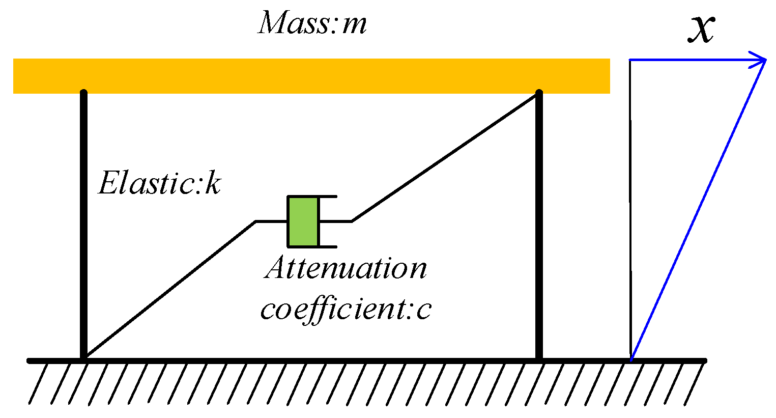
2.1. Analysis Method for Single-Degree-of-Freedom Isolated Structures

In a base isolation structure, the horizontal stiffness of the isolation layer is significantly smaller than the stiffness of the superstructure. During an earthquake, the superstructure experiences a slight displacement and can be regarded as a rigid body in terms of shear translation. Therefore, the structure can be simplified into an SDOF system, as illustrated in Figure 1, which facilitates rapid analysis using the simplified model.

The equivalent model is established by the equivalent linearization method, and the differential equation of motion of the equivalent linear system is

$${\ddot{x}}_{eq}+2{\zeta }_{eq}{\omega }_{eq}{\dot{x}}_{eq}+{{\omega }_{eq}^{2}x}_{eq}=-{\ddot{x}}_g$$

(1)

where ${\zeta }_{eq}$ is the equivalent damping ratio, ${\omega }_{eq}$ is the equivalent period, and $x_{eq}$, ${\dot{x}}_{eq}$, and ${\ddot{x}}_{eq}$ are the displacement, velocity, and acceleration of the equivalent elastic system, respectively.

By simplifying the original structure into an equivalent elastic system for analysis, the goal of simplifying computation for the original structure is achieved. To accurately estimate the seismic peak response of the actual structure with the equivalent linear system, it is essential to establish a reasonable equivalent period (stiffness) and equivalent damping ratio. Typically, these values can be derived from theoretical formulas or by using the secant stiffness at the maximum displacement of an SDOF system to represent the equivalent stiffness, from which the equivalent period can be calculated. The calculation of the equivalent damping ratio is based on the principle that, during one vibration cycle, the damping energy dissipation in the equivalent linear system equals the yielding energy dissipation in the nonlinear system.

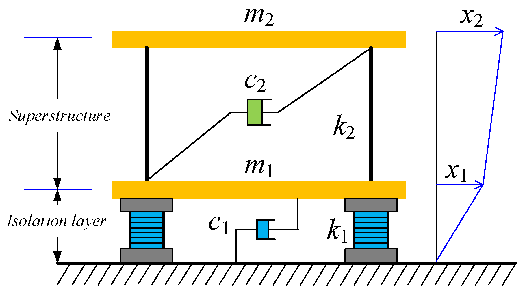
2.2. Analysis Method for Two-Degree-of-Freedom Isolation Structures

A simplified single-degree-of-freedom model can quickly determine the isolation layer parameters required to meet the design goals for a relatively rigid superstructure. When it is necessary to consider the influence of the natural period of the superstructure, a dual-degree-of-freedom system calculation model can be established for the seismic isolation building, as shown in Figure 2. This two-degree-of-freedom (2DOF) system is equivalent to the superstructure as an SDOF system, which is connected in series with the seismic isolation system.

In this model, the damping and stiffness of both the upper building and the seismic isolation system are treated as separate elements. At the same time, the mass is concentrated at the floor level. When the ground produces a movement displacement x_g, the governing equations for the system shown in Figure 2 can be expressed as

$$m_1\left({\ddot{x}}_1+{\ddot{x}}_g\right)+c_1{\dot{x}}_1+k_1{x}_1-c_2\left({\dot{x}}_2-{\dot{x}}_1\right)-k_2\left(x_2-x_1\right)=0$$

(2)

and

$$m_2\left({\ddot{x}}_2+{\ddot{x}}_g\right)+c_2\left({\dot{x}}_2-{\dot{x}}_1\right)+k_2\left(x_2-x_1\right)=0$$

(3)

In order to consider the influence of the circular frequencies of the isolation layer and the upper structure on the overall isolation structure, the following parameters are introduced. Three variables of seismic isolation structure are introduced as follows:

$${\omega }_s=\sqrt{{\displaystyle \frac{k_2}{m_2}}}$$

(4)

$${\omega }_I=\sqrt{{\displaystyle \frac{k_1}{m_1+m_2}}}$$

(5)

$$\mathsf{\gamma }={\displaystyle \frac{m_2}{m_1+m_2}}$$

(6)

where ${\omega }_s$ is the natural frequency when the foundation of the superstructure is fixed; ${\omega }_I$ means that the superstructure is regarded as a rigid body, and the lower mass m₁ and the upper mass m₂ are combined into the natural frequency of a single-degree-of-freedom system; and γ is expressed as the ratio of the mass of the upper mass to the total mass. Solving for ${\omega }^2$,

$${\omega }^2={\displaystyle \frac{1}{2\left(1-\gamma \right)}}\left\{{\omega }_S^2+{\omega }_I^2\mp \sqrt{{\left({\omega }_S^2+{\omega }_I^2\right)}^2-4\left(1-\gamma \right){\omega }_S^2{\omega }_I^2}\right\}$$

(7)

Since ${\omega }^2$ is the first-order and second-order natural frequency from small to large, the negative and positive signs in Equation (7) correspond to the first-order and second-order natural frequencies:

$${\displaystyle \frac{{}_1{}^{ }\omega _{ }^2}{{\omega }_I^2}}={\displaystyle \frac{{\left(\frac{{\omega }_S}{{\omega }_I}\right)}^2+1-\sqrt{{\left(\frac{{\omega }_S}{{\omega }_I}\right)}^4+1+2{\left(\frac{{\omega }_S}{{\omega }_I}\right)}^2-4\left(1-\gamma \right){\left(\frac{{\omega }_S}{{\omega }_I}\right)}^2}}{2\left(1-\gamma \right)}}$$

(8)

In order to find the eigenvector of the first-order natural frequency, the eigenmode vector of the first-order natural circular frequency ω is calculated as

$${}_1{}^{ }\Phi _{ }^{ }={\left\{{}_1{}^{ }\varphi _1^{ }{}_1{}^{ }\varphi _2^{ }\right\}}^T$$

(9)

$$\left[\begin{array}{cc}{\displaystyle \frac{1}{\gamma }}{\omega }_I^2+{\omega }_s^2-{\displaystyle \frac{\gamma }{1-\gamma }}{\omega }^2& -{\omega }_s^2\\ -{\omega }_s^2& {\omega }_s^2-{}_1{}^{ }\omega _{ }^2\end{array}\right]\left\{\begin{array}{c}{}_1{}^{ }\varphi _1^{ }\\ {}_1{}^{ }\varphi _2^{ }\end{array}\right\}=\left\{\begin{array}{c}0\\ 0\end{array}\right\}$$

(10)

where ${\varphi }_{12}/{\varphi }_{11}$ can be calculated using the following equation:

$${\displaystyle \frac{{}_1{}^{ }\varphi _2^{ }}{{}_1{}^{ }\varphi _1^{ }}}={\displaystyle \frac{1}{1-\frac{{}_1{}^{ }\omega _{ }^2}{{\omega }_S^2}}}$$

(11)

Define $T_1$ as the first period of the overall isolation structure; define $T_I$ as the period when only the isolation layer’s stiffness is considered and the upper structure is a rigid body; and define $T_s$ as the stiffness of the upper structure when it is not in isolation.

Equation (7) reflects the ratio $T_I/T_S$of the natural vibration period of the isolation system to that of the building, along with the change in the main natural period and relative displacement of the 2DOF system. Figure 3 illustrates the ratio of the natural vibration period of the 2DOF system to that of the isolation system when $T_I/T_S$ changes within the range of 1–100. The modal amplitude is displayed in the figure, which is represented by the relative deformation of upper mass to lower mass when lower mass is the standard deformation 1. Both graphs plot the results of three cases where γ is 0.5, 0.7, and 0.9.

From Figure 3, it is evident that $T_1/T_I$ is close to 1.0 when $T_I/T_S>3$—that is, the first-order natural period is very close to the natural period of the isolation layer, and the change in the mass ratio has little effect on the result. In Figure 4, within the same area, the relative displacement between the upper mass and lower mass is nearly zero, indicating a behavior similar to that of a rigid body. If $T_I/T_S$ is close to or greater than 3, the nature of the seismic isolation structure is close to a rigid body, which can be simplified to an SDOF model.

$${\displaystyle \frac{T_I}{T_s}}={\displaystyle \frac{2\pi \sqrt{\frac{m_1+m_2}{k_1}}}{T_s}}$$

(12)

The equivalent period k₁ is calculated as follows:

$$k_1=k_d+{\displaystyle \frac{Q_d}{\delta }}$$

(13)

where k_d is the post-yield stiffness of the seismic isolation layer, Q_d is the yield strength of the lead core, and δ is the displacement of the seismic isolation layer.

The post-yield circular frequency ${\omega }_d$ and the flexion weight ratio $R_{yw}$ are

$${\omega }_d={\displaystyle \frac{2\pi }{T_d}}=\sqrt{{\displaystyle \frac{k_d}{m_1+m_2}}}$$

(14)

$$R_{yw}={\displaystyle \frac{Q_d}{\left(m_1+m_2\right)g}}$$

(15)

$${\displaystyle \frac{T_I}{T_S}}={\displaystyle \frac{2\pi }{T_s\sqrt{\frac{4{\pi }^2}{T_d^2}+\frac{R_{yw}g}{\delta }}}}$$

(16)

Since $T_I/T_S>3$,

$${\mathrm{T}}_{\mathrm{S}}\sqrt{{\displaystyle \frac{4{\mathsf{\pi }}^2}{{\mathrm{T}}_{\mathrm{d}}^2}}+{\displaystyle \frac{R_{yw}g}{\delta }}}\le {\displaystyle \frac{2\pi }{3}}$$

(17)

The value range of the post yield period is

$$T_d\ge {\displaystyle \frac{2\pi T_s}{\sqrt{{\left(\frac{2\pi }{3}\right)}^2-\frac{R_{yw}g}{\delta }{T}_s^2}}}$$

(18)

2.3. Analysis Method for Multi-degree-of-freedom Isolation Structure

To perform fast elastic–plastic analysis of the isolated structure, evaluate its seismic response, and predict its seismic performance, this paper simplified the isolated structure to the multi-degree-of-freedom (MDOF) shear model, as illustrated in Figure 5. To simulate the elastic–plastic performance of the upper multi-story frame structure of the seismic isolation structure, this paper adopted the modified Takeda model as the hysteretic model [31,32]. This model is applicable to frame structures where layer shear deformation is dominant and the overall structure mainly undergoes translational motion. As shown in Figure 6, the initial stiffness is K₀, and the degenerate stiffness is determined by multiplying the initial stiffness by the stiffness reduction factor. The strengths that characterize the cracking and yielding of the component are P₁ and P₂, with their corresponding deformations denoted as D₁ and D₂. The arrows illustrate the loading and unloading hysteresis trend.

To verify the reliability of the modified Takeda hysteresis model, the results of repeated loading tests on two reinforced concrete columns represent in [33] are used for comparison; the parameters of the components are also detailed in [33]. The hysteresis results from the simulations based on the modified Takeda model and the published test results are illustrated in Figure 7. It is evident that the skeleton curves of the two test components are similar to the calculation results obtained from the program, thereby demonstrating the reliability of the modified Takeda hysteretic constitutive model.

Moreover, while addressing the simplified model of the superstructure, it is vital to focus on simulating the mechanical properties of the seismic isolation layer. The restoring force model of the rubber bearing is categorized into two directions, namely the axial tension and compression performance and the bearing shear mechanical properties, as illustrated in Figure 8. It is important to note that the mutual influence of axial and tangential mechanical properties is not considered in the MDOF elastic–plastic simplified model.

Consider the loading conditions of the lead–rubber bearing as described in [34] for test calculations. The bearing’s diameter is 600 mm, the lead core’s diameter is 140 mm, and the total height of the bearing is 269 mm. As shown in Figure 9, the simulated hysteresis results closely align with the test curve. The numerical method effectively captures the strengthening phenomenon of the support. When the shear deformation of the support exceeds about 250%, the rubber stiffens, and its stiffness increases. This paper employs a three-fold line mechanics model considering the hardening effect of the bearing.

Since the dynamic response of the superstructure is directly influenced by the dynamic response and failure modes of the seismic isolation bearing, it is essential to comprehensively evaluate the seismic performance of the seismic isolation bearing and the superstructure in the performance design of the RC base isolation frame structure and to integrate the sub-components effectively.

3. Performance Evaluation of Seismic Isolation Frame Structures

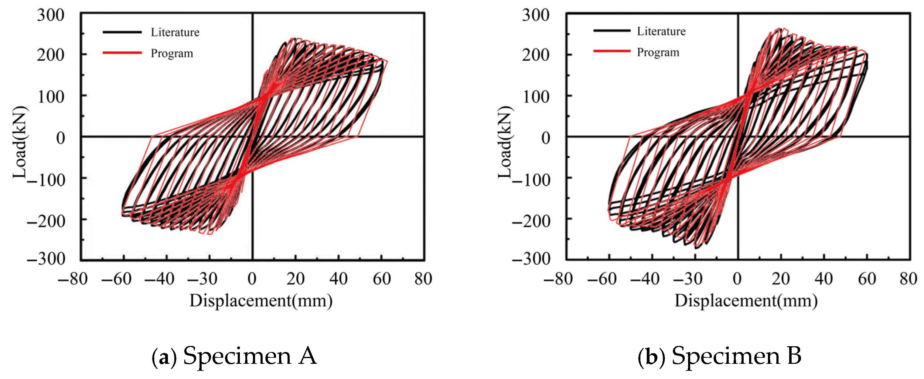
3.1. Classification of Upper Structure Damage Levels

It is essential to classify the seismic performance level of the structure. According to the Chinese code GB50011 [35], the seismic performance objectives are divided into four levels (

Table 1. Seismic performance objectives of structure.

Performance Objective	Earthquake Level
	Frequent Earthquake	Fortification Earthquake	Rare Earthquake
A	1	1	2
B	1	2	3
C	1	3	4
D	1	4	5

). Additionally, the allowable five damage levels of the structures, divided according to the combination of the four performance objectives and the three seismic levels, are shown in

Table 2. Overall structural performance level.

Performance Index	Deformation Limit
Safe	The deformation is less than or slightly greater than the elastic displacement limit.
Superficial damage	The deformation is less than twice the elastic displacement limit.
Mild damage	The deformation is less than three times the elastic displacement limit.
Moderate damage	The deformation is about four times the elastic displacement limit.
Serious damage	The deformation is less than 0.9 times the plastic displacement limit.

.

According to the reference standards, the displacement limits for different structural types are stipulated in Table 2, providing the basis for defining the overall structural performance levels. Taking the frame structure as an example, the limit value of the elastic inter-story displacement angle under the action of moderate earthquakes in the specification is 1/550, and the limit value of the elastic–plastic inter-story displacement angle under the action of rare earthquakes is 1/50. For the shear wall structure, the limit value of the elastic inter-story displacement angle under the action of moderate earthquakes is 1/1000, and the limit value of the elastic–plastic inter-story displacement angle under the action of rare earthquakes is 1/120.

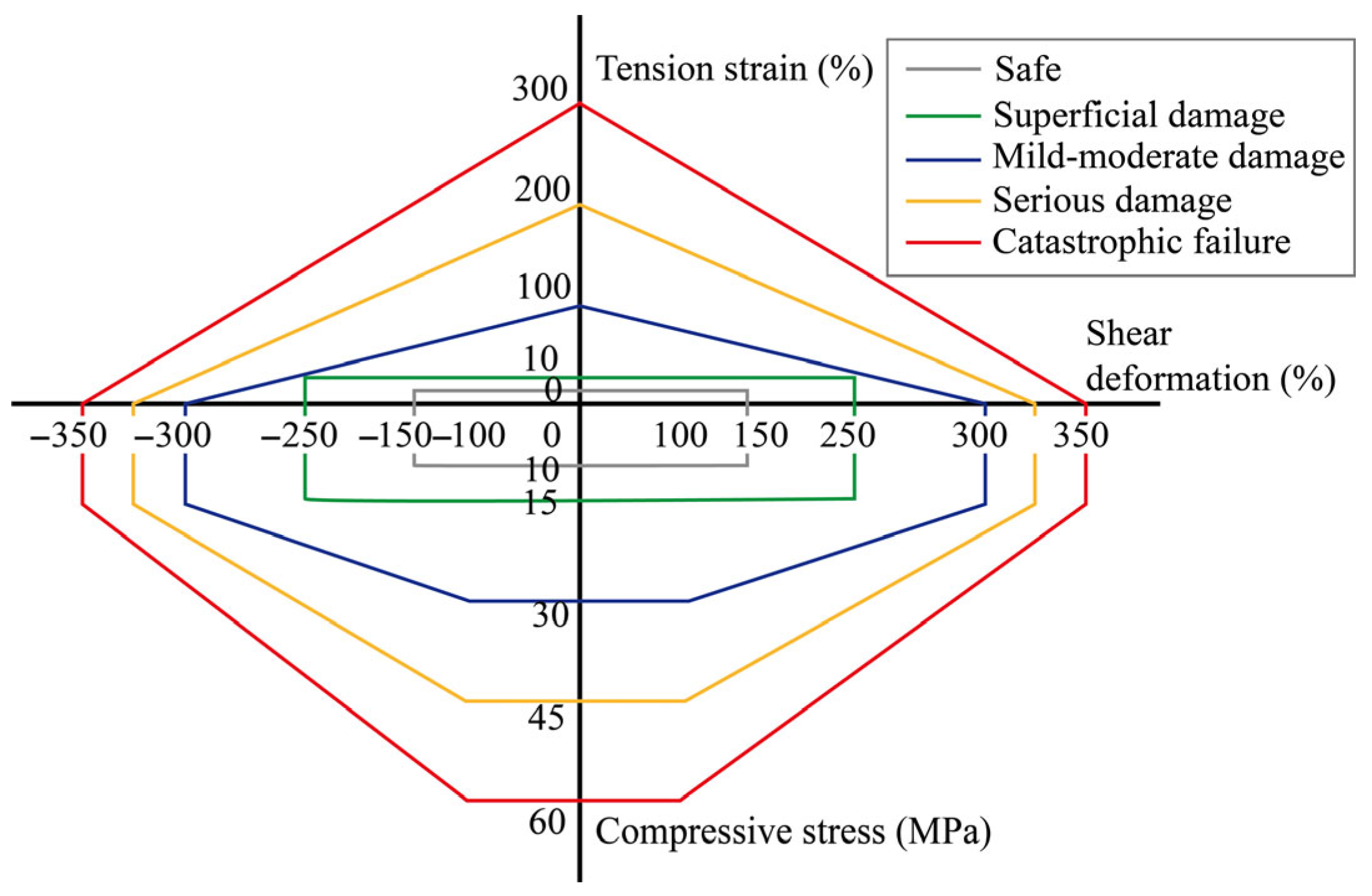
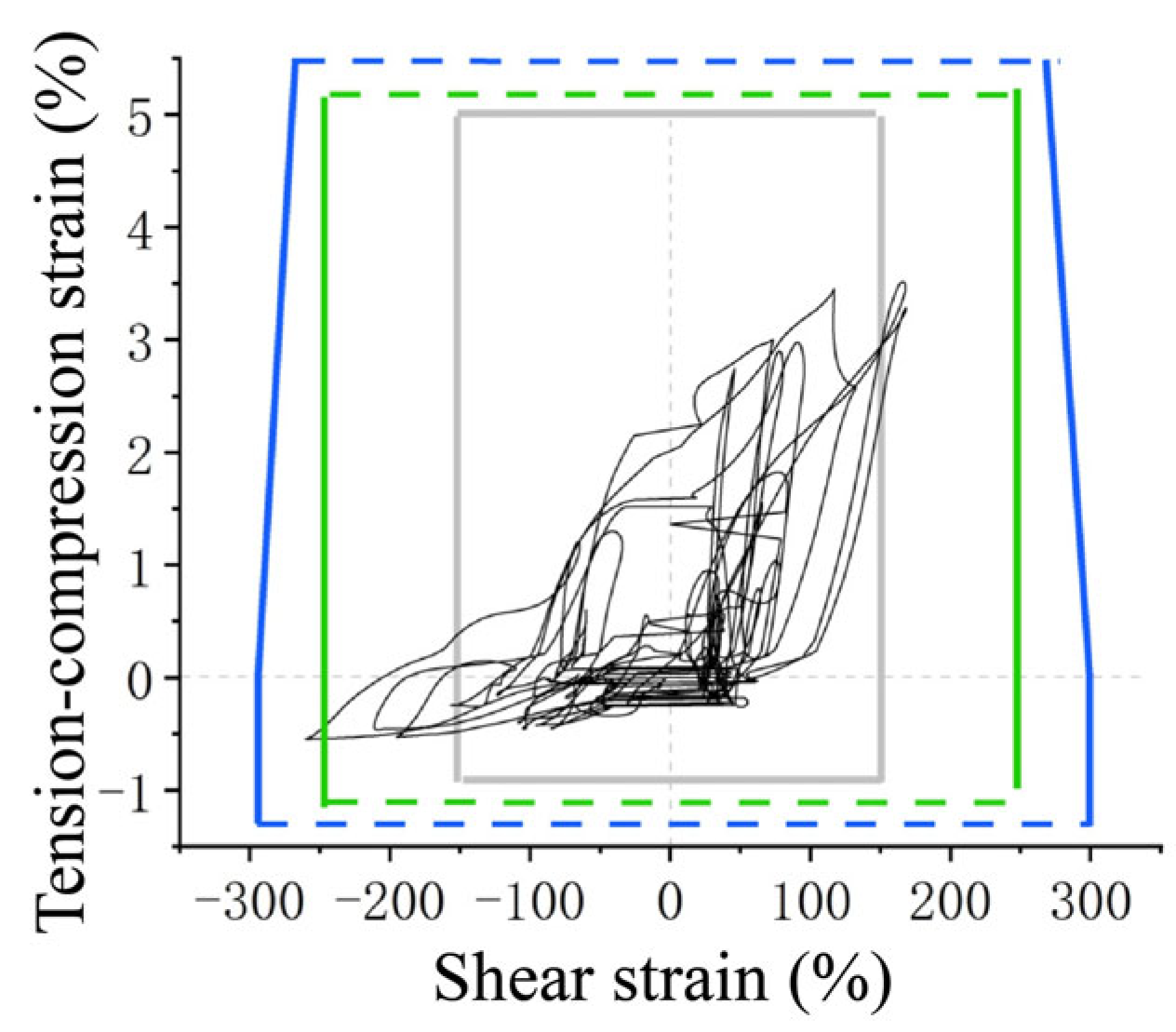
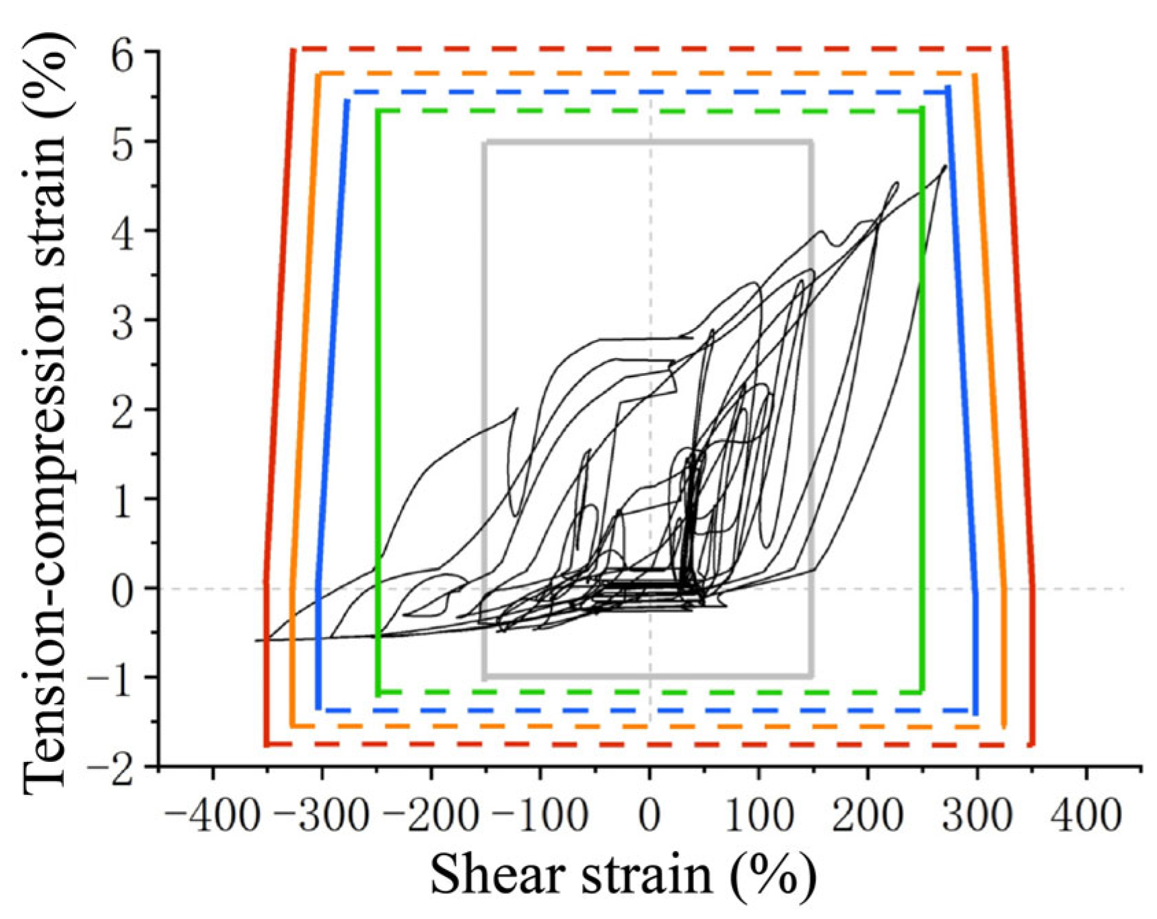
3.2. Classification of Seismic Isolation Bearing Damage Levels

In addition to calibrating the damage indicators of the superstructure, components, and materials, it is essential to assess the damaged state of the rubber bearings within the isolation layer. The mechanical behavior of rubber bearings becomes increasingly complicated under the influence of vertical pressure, horizontal shear, and bending moments. Generally, the deformation of the isolation bearings is a key factor in determining the damage to the isolation layer. As the seismic isolation bearing approaches its limit state, it experiences the coupling effect of the forces in all directions, making it more challenging to predict damage failure, particularly when the bearing is largely deformed. To determine the ultimate performance of the seismic isolation bearing under large deformation and to classify its damage performance level, this section compiles failure performance test samples of 102 rubber isolation bearings from previous research.

The statistics relating to the compression–shear failure test data, including the relationship between the ultimate shear strain of the bearing and the diameter (D) and the second shape factor (S2), are illustrated in Figure 10 and Figure 11. Generally, during the compression–shear test, the horizontal stiffness of the seismic isolation bearing is stable when the shear strain is less than 250%. However, as the shear deformation continues to increase after the shear deformation exceeds 250% to 300%, the bearing begins to harden, resulting in a sudden rise in horizontal stiffness. Moreover, as shown in Figure 11, the limit shear strain tends to increase with an increase in the second shape factor S2. This indicates that bearings with a higher second shape factor provide a greater safety margin. Theoretically, the second shape factor reflects the deformation capacity and stability of the seismic isolation bearing. A smaller second shape factor indicates poorer stability under compression, making the support more susceptible to buckling. Overall, if the second shape factor of the seismic isolation support exceeds 4, the limit shear strain can reach 350%, with that for most bearings exceeding 400% and the maximum potentially surpassing 700%.

As shown in Figure 12, the ultimate axial compression bearing capacity of the seismic isolation bearing can exceed 60 MPa. To achieve a higher ultimate axial compression stress of 90 Mpa, the ratio of the steel plate to the rubber thickness of the rubber bearing must be greater than 0.4. According to the compression test conducted by Liu et al. [36], the bearing compressive stress ranges from approximately 80% to 90% of the ultimate compressive stress before entering the inelastic state. The elastic compressive strain is 9%, which is about one-quarter of the ultimate compressive strain.

In the isolated structure, the deformation stability of the laminated rubber bearing is crucial, and it is essential to minimize the bending deformation of the bearing. Figure 13 illustrates the relationship between the compression stress and shear deformation of the bearing with the second shape factor S2 = 3~6. It is observed that when the shape factor is low (S2 = 3~4), the bearing is susceptible to instability failure as shear deformation and compression stress increase. Conversely, when the stress increases, the bearing is prone to instability failure. When the second form factor is large (S2 = 4~6) and the vertical compressive stress is low, an increase in the shear deformation leads to shear failure as the primary failure mode. However, for bearings with a higher second shape factor, buckling failure can also occur when the compressive stress exceeds 25 Mpa, indicating that these bearings are also vulnerable to buckling under increased shear deformation and higher compressive stress. As illustrated in Figure 13, when the diameter of the bearing remains constant, the shear strain is relatively discrete. For instance, a bearing with a diameter of 200 mm has a limit value for the shear strain ranging from 200% to 700%. The code stipulates 0.55 times the rubber bearing diameter to define the limit of the shear strain; however, this calculated value may significantly deviate from the actual limit strain.

Tensile stress and tensile strain can be used to evaluate the tensile performance of bearings. The current design code uses tensile stress to specify the allowable design limit of the tensile direction of the bearing. The test results for the bearing in the tensile direction showed that the support characteristics differ between the compression and tensile directions. When the tensile stress of the rubber bearing is minimal, the tensile deformation is very large. This occurs because, during an earthquake, the bearing undergoes bending and deformation due to tensile and shear forces, which makes it challenging to transmit the load evenly to the interior of the bearing. Therefore, using tensile strain as a performance index for evaluating the tensile mechanical performance of the bearing is a more effective approach.

Ref. [37] presents the theoretical relationship curve between the tensile limit deformation and the shear strain of the laminated rubber bearing, as well as the undamaged test results of various types of bearings. Figure 14 illustrates that the rubber bearing can fail either in tension or buckle under a tension–shear condition. As the shear strain increases, the limit tensile strain of the rubber bearing gradually decreases. When the shear deformation is large, the support may experience buckling; conversely, under smaller shear deformation, the bearing initially yields before ultimately failing due to the tensile force. In the pure compression test, the limit tensile strain of the bearing can reach more than 300%, with a maximum of 500%.

The data curve of the test conducted by [31] is presented in Figure 15. During the limit tensile test, the bearing exhibits greater tensile stiffness of the bearing in the elastic stage. When the tensile stress is 1–2 Mpa, the rubber bearing begins to yield. This occurs at a tensile strain of 5% to 10%, marking the transition to an inelastic state. Once the laminated rubber bearing enters this inelastic state, the tensile stiffness drops suddenly, and the tensile strain increases rapidly. The bearing fractures when the tensile strain exceeds 300%.

The compression–shear failure limit curve of the rubber bearing is given by design codes [38], as shown in Figure 16.

In the preceding sections, the compressive stress, tensile strain, and horizontal shear strain of the bearing were used as the force and deformation indexes to evaluate the damage performance. Through the statistical analysis of test phenomena and data, the influence of the bearing parameters on the limit deformation of the bearing and the relationship between these parameters and the failure mode are analyzed, and the failure limit curves (Figure 16) are established by integrating the statistical trends of ultimate shear strain with bearing diameter and shape factor (Figure 10 and Figure 11), the compressive stress–shear deformation failure modes (Figure 13), and the tensile-shear limit deformations (Figure 14 and Figure 15). Drawing from theoretical frameworks and current design codes [38], the tensile-shear failure limit and the compression–shear failure limit are established. We divide the performance level of the bearing and describe the damage under each level state (

Table 3. Damage description of laminated rubber bearings under different performance states.

Performance Level	Damage Situation
Safe	The bearing is in an elastic state.
Superficial damage	There is a small residual deformation in the rubber layer of the bearing. The tensile deformation may enter the yield stage, but it does not yield.
Mild-moderate damage	Bearing may exhibit a hardening phenomenon, limiting bearing displacement. If tensile yield occurs, the tensile stiffness of the bearing decreases rapidly, and a negative pressure state may form inside the rubber of the bearing, resulting in empty holes and damage.
Serious damage	The rubber layer at the connection between the bearing sealing plate and the rubber may be torn up: the bearing hardening phenomenon is evident, and the shear force is increased, increasing the seismic response of the upper floor; or the bearing buckling phenomenon.
Catastrophic damage	The warping deformation continues to develop, and the rubber layer is about to break off, and shear failure occurs.

).

4. Fragility Analysis of Isolated RC Frame Building

This section presents a case study of an isolated RC frame building aimed at verifying the validity and accuracy of the equivalent linearization displacement method. An analysis program was developed based on the principles outlined in Section 2.3, and the results were compared with those obtained from general numerical analysis software (Perform3D version 8). Additionally, to understand the vulnerability of the isolated structure, a statistical analysis was conducted on the damage levels of the isolation layer and upper structure under increasing seismic acceleration.

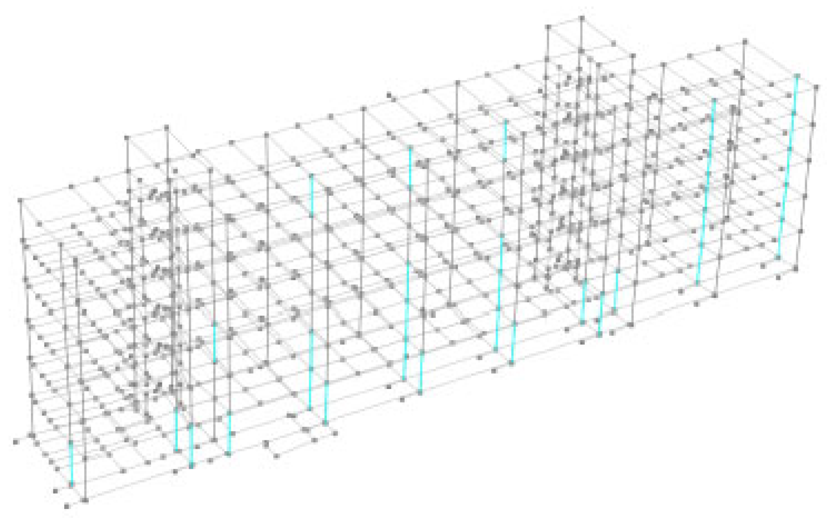
4.1. Overview of the Structural Model

This building serves as a teaching facility for a school, as depicted in its architectural rendering in Figure 17. The building has six floors above ground level, with the bottom floor located underground. The height of the structural roof elevation reaches 22.3 m, while the dimension of the rectangular plane is 69.8 m × 10.7 m, resulting in a structural aspect ratio of 2.08. The building uses a reinforced concrete frame structure. It is designed to withstand seismic fortification intensity of 8 degrees, with a peak design seismic acceleration value of 0.3 g. The characteristic site period is 0.55 s, and the wind pressure is observed to be 0.8 kN/mm². The non-isolation model of this structure was analyzed. The total mass of the structure was found to be 6252 tons. The first three natural vibration periods were 0.846 s, 0.761 s, and 0.689 s.

4.2. Design of Seismic Isolation Layer

In calculating and analyzing the base isolation structure using the SDOF design method, the yield force of the seismic isolation layer required to resist wind was calculated to be 4500 kN, as specified. We let the period after yielding of the seismic isolation layer T_f = 2.8 s, and then the stiffness of the seismic isolation layer after yielding was k₂ = 36.59 kN/mm. The detailed parameters of the isolation bearings are provided in

Table 4. Isolation bearing parameter.

Model	LNB 700	LRB 800-1	LRB 800-2	LRB 900
Number	5	8	7	10
Height (mm)	304	337	315	351
Total thickness of the rubber layer (mm)	140	156	144	175
Vertical stiffness (106 kN/m)	2.70	3.04	2.74	3.59
Equivalent horizontal stiffness (kN/m)	1100	2030	2870	2640

LNB represents linear natural rubber bearings, LRB represents lead–rubber bearings, and the numbers following the characters indicate the bearing size.

. From the dynamic analysis of the 2DOFs base isolation structure presented in Section 2, it is evident that the isolation period is extended by nearly three times. Consequently, the upper structure of the isolation structure can be treated as a rigid body for shear-type translation under the action of a horizontal earthquake.

After the bearing selection was completed, the election results were checked, which mainly included the vertical pressure check of the seismic isolation bearing, the wind resistance check, the eccentricity of the isolation layer check, and the elastic restoring force check. All of these checks met the requirements of the design codes [38]. The layout and quantities of different types of isolation bearings are presented in Figure 18.

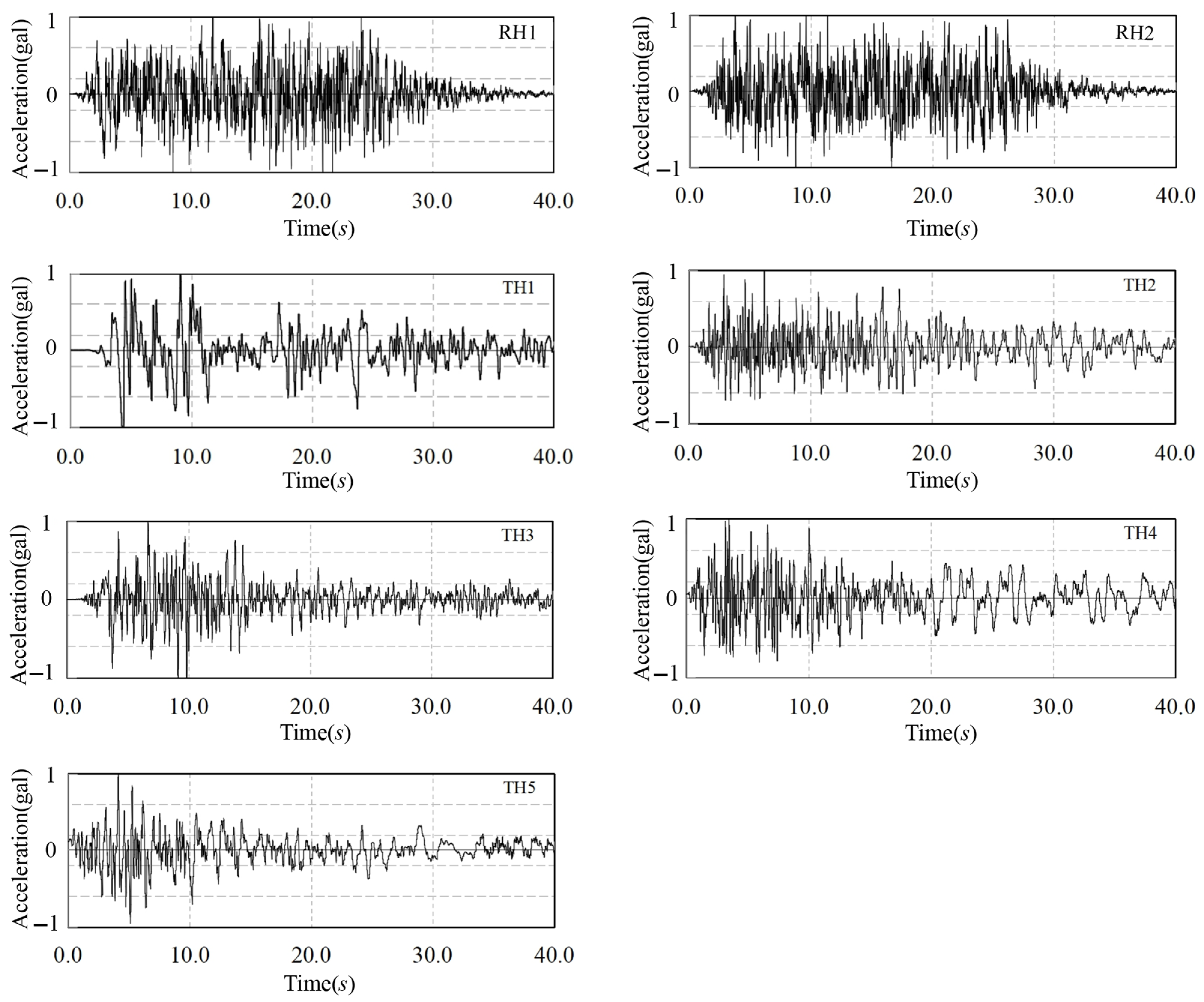
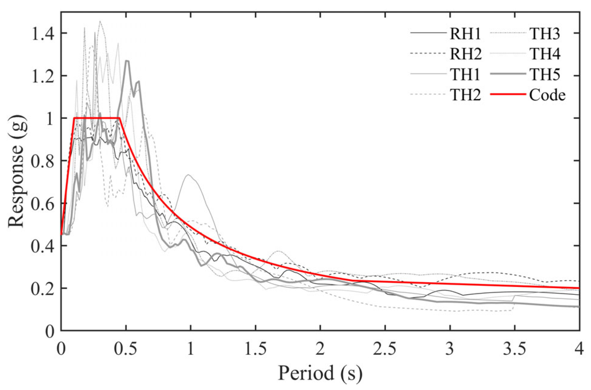
4.3. Design Results and Model Response Verification

The time history analysis of this project selected seven seismic waves, including two artificial waves, RH1-RH2, and five natural waves, TH1-TH5, as shown in Figure 19 and Figure 20. This structure employed numerical analysis software to perform calculations and analysis on both non-seismic and seismic isolation structures. In the numerical model, the mechanical properties of the seismic isolation bearing were simulated by connecting element properties.

When the peak value of the fortified earthquake acceleration input reached 300 Gal, a time history analysis was conducted under this fortified earthquake action using both a non-isolated model and an isolated model to obtain the inter-story shear force. The average value of the seven seismic wave results was taken for each floor. According to

Table 5. Maximum floor shear ratio of isolated structure and non-isolated structure.

Story	X Direction	Y Direction
Roofing	0.165	0.150
6	0.204	0.190
5	0.233	0.220
4	0.262	0.242
3	0.300	0.268
2	0.333	0.303
1	0.361	0.342
0 (Isolation layer)	0.322	0.308

, the horizontal seismic reduction factor is 0.361, indicating that the design results have apparent isolation effects.

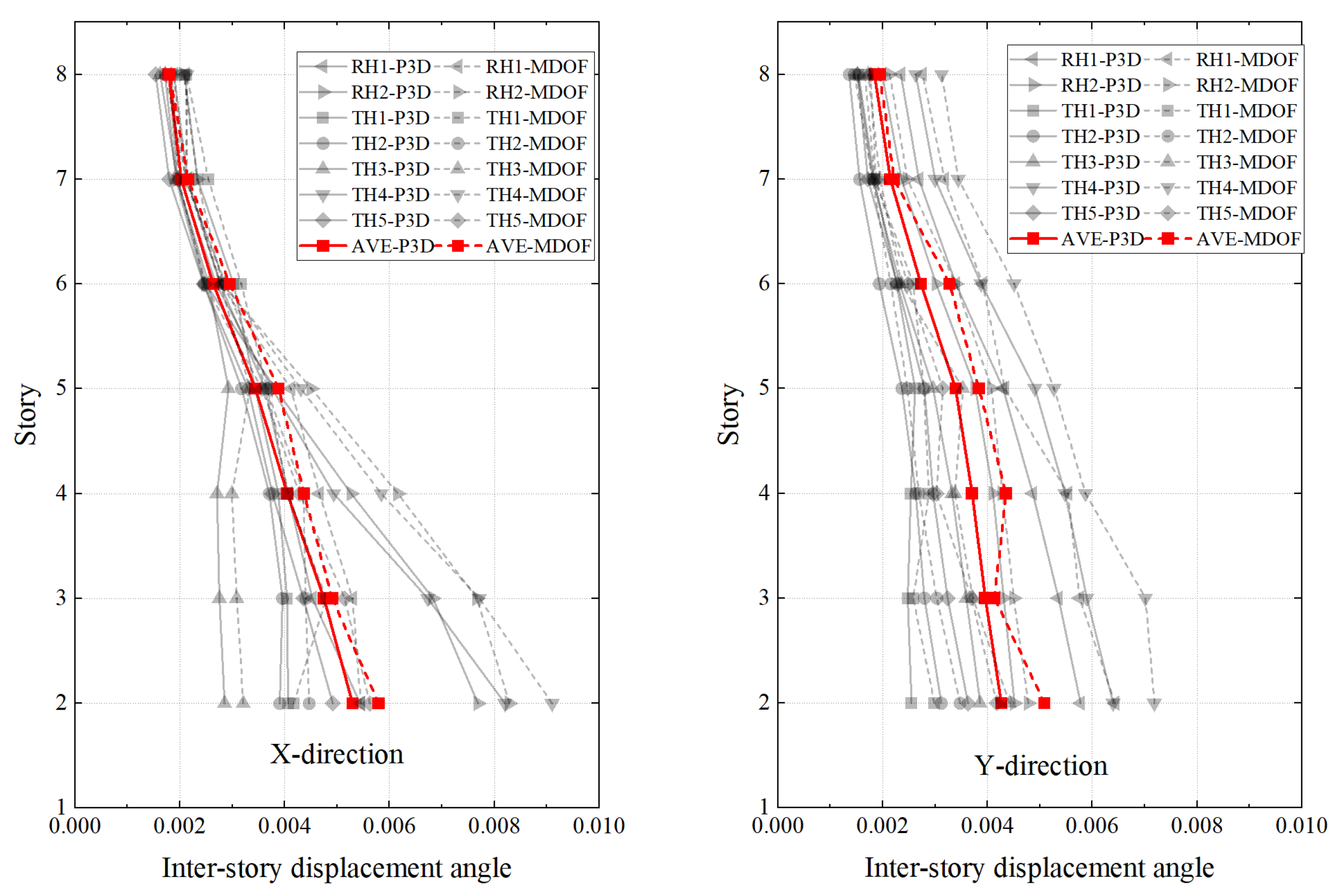
4.4. Comparison of Results Between MDOF Model and Frame Model

Under the RH1-X condition (“-X” indicating input along the global X axis), the finite element software Perform-3D (P3D, version 8) was used to analyze the dynamic elasticity and elastic–plastic time history. The results were compared with the elastic and elastic–plastic calculations. The finite element software was used to perform elastic and elastic–plastic analysis. The resulting hysteresis curve and top displacement time history results of the seismic isolation layer are similar to the calculation and analysis results of the program, as demonstrated in Figure 21. This indicates that the program can efficiently perform fast elastic–plastic calculation and analysis of seismic isolation structure. Furthermore, the program accommodates the hardening displacement of the isolation layer to account for the large deformation stiffness hardening of the support. Under the TH4-X seismic condition, which features an acceleration of 0.84 g, the hysteresis curve of the numerical model for the isolation layer aligns with the calculated hysteresis curve for the seismic isolation layer, as illustrated in Figure 22. We used finite element software to perform elastic–plastic time history analysis on refined models. Although more detailed performance evaluations can be performed at the material or component level, when efficient design and evaluation of seismic isolation structures are required, the MDOF simplified model can save considerable time and effort.

Figure 23 compares the inter-story drift angles, which are crucial in evaluating structural response. The drift angles calculated by the MDOF model exhibit a relatively small error compared to the results of the finite element analysis, at approximately around 10%. Since the MDOF model adopts a more conservative approach, the calculated drift angles are consistently higher than those derived from the finite element analysis.

The data errors associated with the top displacement time history of the structure, the hysteretic curve of the seismically isolated story, and the interlayer displacement angle are all minimal. This suggests that the data required for accurate vulnerability assessment can be effectively derived using the MDOF model.

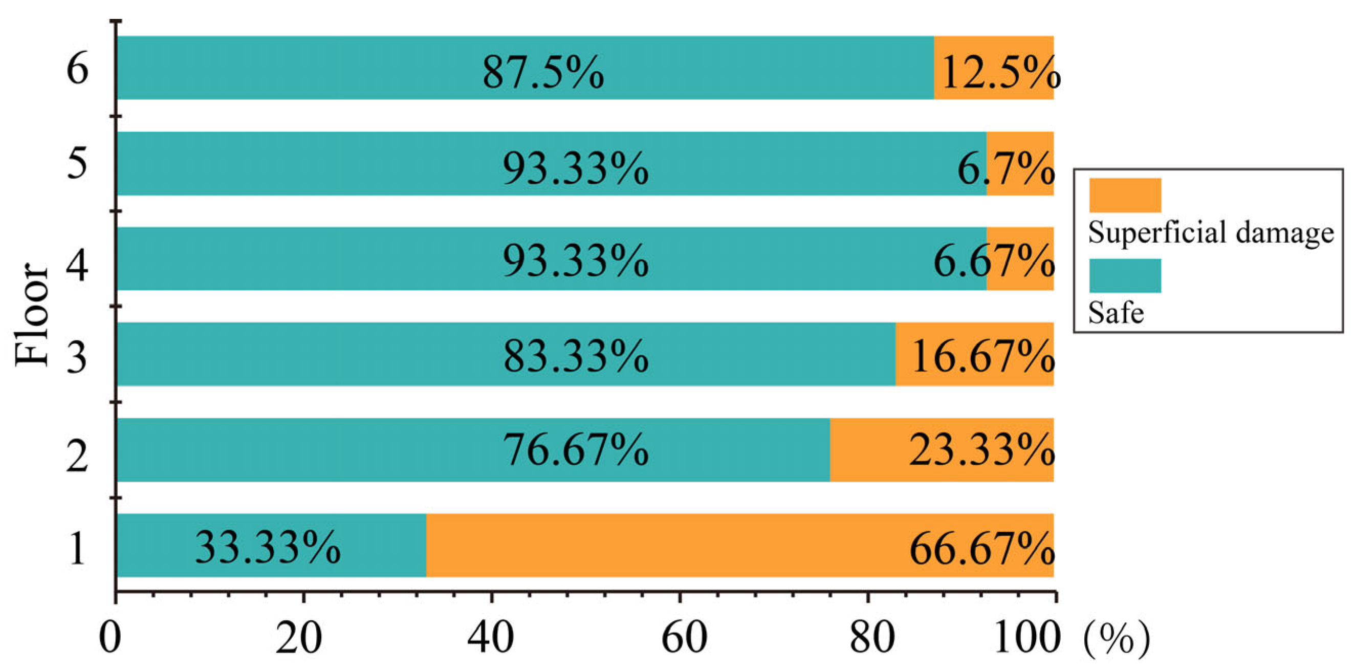
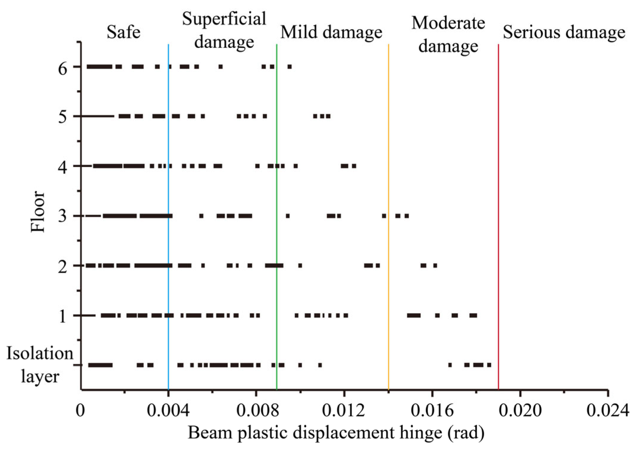
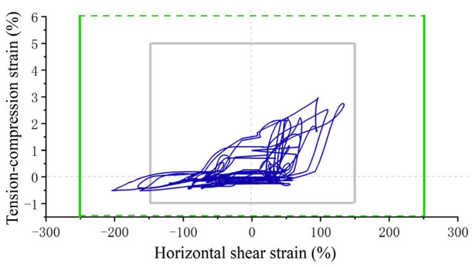
4.5. Damage Analysis of the Isolation Layer and Structural Components

Based on the ASCE/SEI 41-17 [39] specification, the damage grade of concrete components is determined. The plastic damage of the frame columns in the main X direction is lower than that observed in the main Y direction. Under the TH1 earthquake condition, the damage to the frame column is minimal, with the majority remaining in a non-damaged state. Conversely, the frame column is the most severely damaged during the TH4 earthquake condition, as illustrated in Figure 24. The blue lines denote that the component has already developed partial plastic rotation, indicating the initiation of inelastic deformation. However, it is noteworthy that, under all seismic conditions, the frame columns, functioning as vertical members, exhibited only slight damage. The shear demand capacity ratio is the ratio of the maximum shear force experienced by the frame column to the design value and standard value of the frame column’s shear bearing capacity, corresponding to the shear elastic demand capacity ratio and the shear yield demand capacity ratio.

Figure 25 illustrates the plastic deformation of frame columns on each floor under the envelope values of seven sets of seismic conditions. The column damage basically decreases with the increase in the floor height, and the frame columns with slight damage mainly appear on the first floor.

Energy-dissipating beams experience the least amount of damage under TH1-X earthquake conditions, with only minimal damage observed in some beams. In contrast, the damage to the beam members was most severe under TH4-Y earthquake conditions, with a few beams exhibiting light to moderate damage but no more severe damage. During rare earthquakes, large plastic deformations occur in these energy-dissipating components. To understand the distribution of plastic displacement angles of beam components along with floors, the plastic displacement angle value is counted, as illustrated in Figure 26. In summary, during the occurrence of rare earthquakes, reinforced concrete beams can successfully meet the performance target B requirement of “slight damage and a small part of moderate damage” for energy-consuming components, even under the most severely damaged seismic conditions.

Since the seismic isolation structure mainly undergoes horizontal translation, the deformation of each bearing in the isolation layer is essentially uniform. Thus, the K1 bearing is chosen as the representative for damage assessment. The horizontal shear strains of the K1 bearing under TH4 seismic conditions, combined with the time history curves of both tensile and compressive strains, is superimposed on the bearing damage performance level diagram, as shown in Figure 27.

The analysis reveals that the seismic isolation bearing does not appear to cause large deformation damage under the acceleration of rare earthquakes. To evaluate the seismic performance of the isolation structure with large deformation stiffness and hardening, the acceleration will be 0.62 g, 0.73 g, and 0.84 g. An incremental dynamic elastic–plastic analysis of the seismic isolation structure will be conducted. Figure 28, Figure 29, Figure 30 and Figure 31 show the damage of the K1 bearing under different seismic accelerations. The colors of the rectangles indicate bearing damage levels, matching the classification in Figure 16.

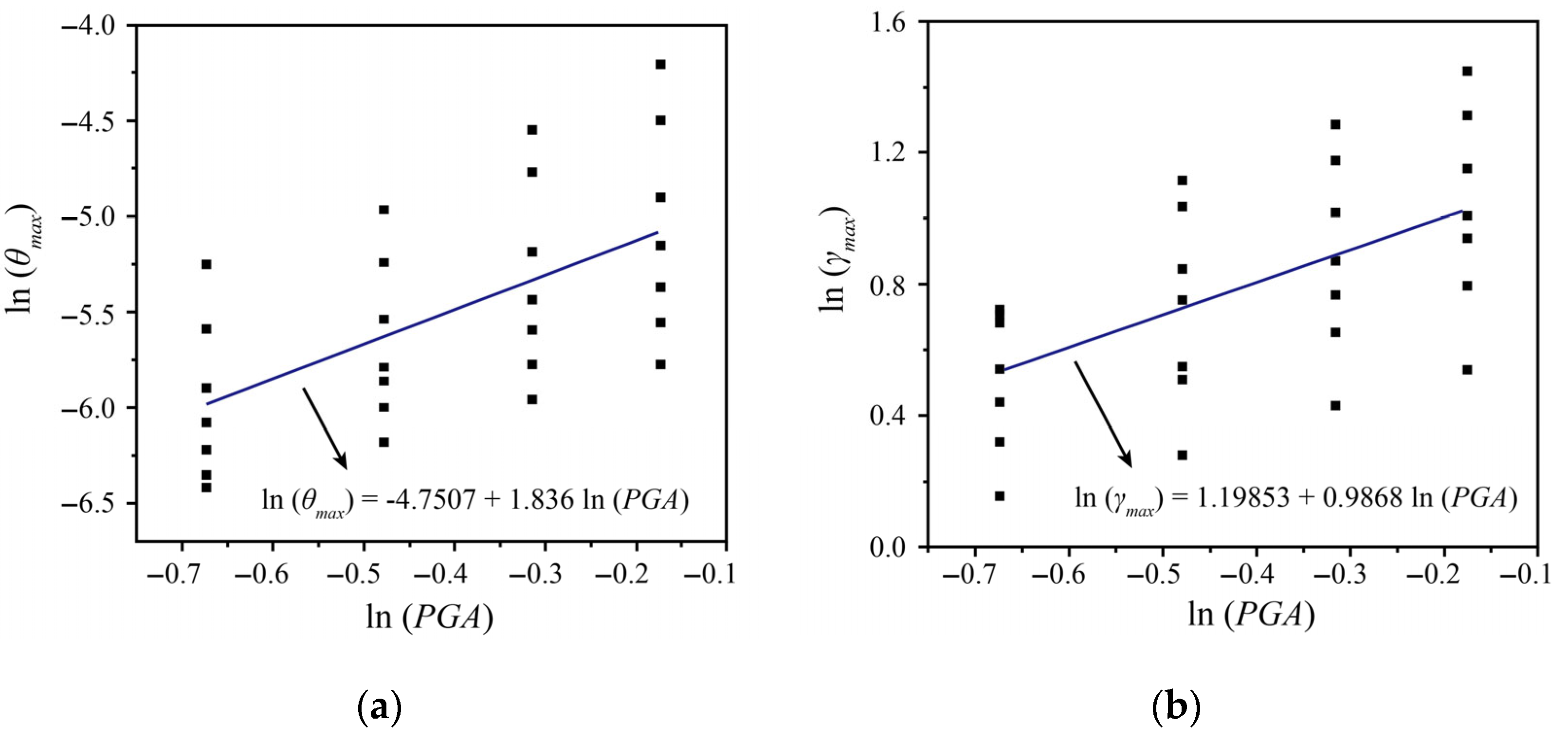
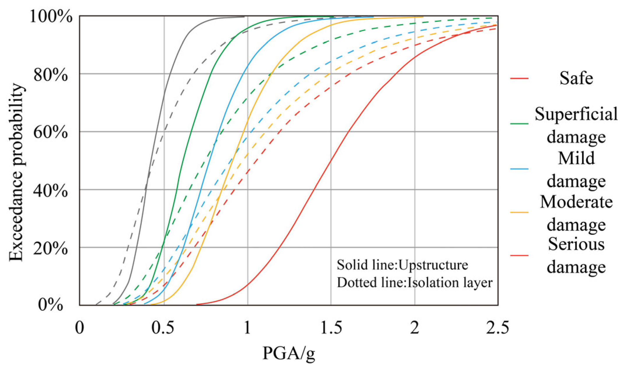
4.6. Seismic Fragility Analysis of Isolated Structures

Seismic vulnerability reflects the probability of a structure exceeding a certain damage state under the influence of different seismic levels and also reflects the seismic performance of the structure. Incremental dynamic analysis (IDA) involves multiplying the ground motion by different amplitude modulation coefficients to obtain the corresponding structural dynamic response. Peak ground acceleration (PGA) is used to characterize the intensity of ground motion. To integrate the seismic vulnerability of the isolation layer and the superstructure of the system, the maximum inter-story drift angle (θ_max) of the upper structure is selected as the demand parameter, and the seismic isolation layer takes the maximum shear strain (γ_max) as the required parameter. The structural deformation index limits and bearing shear deformation index limits are shown in

Table 6. Damage state and damage index limit of superstructure and isolation layer.

Damage State	Basically Intact	Slight Damage	Mild Damage	Moderate Damage	Relatively Severe Damage
Inter-story drift limit value θ	1/550	1/275	1/183	1/137	1/55
Shear strain limit value of isolation layer γ	150%	250%	300%	325%	350%

.

Seven ground motions were used to modulate the amplitude to 0.51 g, 0.62 g, 0.73 g, and 0.84 g for incremental dynamic elastic–plastic analysis of the seismic isolation structure. To validate the lognormal distribution assumption for PGA and structural damage indicators (θ_max, γ_max), Kolmogorov–Smirnov (K-S) tests were conducted. The results showed that the D-statistics for PGA, θ_max, and γ_max were 0.12, 0.09, and 0.11, respectively, with corresponding p-values of 0.34, 0.57, and 0.42, all exceeding the significance level of 0.05. Since the PGA and structural damage indicators θ_max and γ_max conform to the normal distribution, the logarithm of PGA, θ_max, and γ_max is taken based on the IDA results, and linear regression statistics are performed. The fitting results are shown in Figure 32.

The demand expressions of the superstructure and the seismic isolation layer are as follows:

$$\begin{gathered} \mathrm{l}\mathrm{n}\left({\theta }_{\mathrm{m}\mathrm{a}\mathrm{x}}\right)=-4.7507+1.836\mathrm{l}\mathrm{n}\left(PGA\right) \\ \mathrm{l}\mathrm{n}\left({\gamma }_{\mathrm{m}\mathrm{a}\mathrm{x}}\right)=1.19853+0.9868\mathrm{l}\mathrm{n}\left(PGA\right) \end{gathered}$$

(19)

The vulnerability curve indicates the conditional probability that the structural deformation demand D exceeds the structural limit deformation capacity C under different seismic intensity indicators:

$$P_f=P\left(D/C\ge 1\right)$$

(20)

Since both D and C conform to the normal distribution, the probability of exceeding the superstructure under a certain seismic level is

$$P_f\left(PGA\right)=\Phi \left({\displaystyle \frac{\mathrm{l}\mathrm{n}\left({\theta }_{\mathrm{m}\mathrm{a}\mathrm{x}}/{\theta }_c\right)}{\sqrt{{\beta }_c^2+{\beta }_d^2}}}\right)$$

(21)

The vulnerability curve takes the seismic peak acceleration as the independent variable, and the average standard deviation ${\beta }_z=\sqrt{{\beta }_c^2+{\beta }_d^2}$ can be 0.5, while φ is the standard normal distribution function.

$$\Phi ={\displaystyle \frac{1}{\sqrt{2\pi }}}{\int }_{-\infty }^x\mathrm{e}\mathrm{x}\mathrm{p}\left(-{\displaystyle \frac{t^2}{2}}\right)dt$$

(22)

Fitting straight lines between the damage limits of the structure’s different performance levels and the ground motion requirements is substituted into the formula to obtain the exceedance probability of the structure. The vulnerability curves of the upper structure and the isolation layer under different limit damage states of the seismic isolation structure are shown in Figure 33. Under the same intensity of ground motion, the exceedance probability of the superstructure and the seismic isolation layer, ranging from no damage to severe damage, decreases. The fragility curve of the superstructure and the fragility curve of the seismic isolation layer show a staggered upward trend, and the growth rate of the two is also different in the range of varying ground motion intensities. As the PGA increases, the exceedance probability of the seismic isolation layer is first higher and then lower than that of the superstructure in states ranging from no damage to moderate damage. In the more severely damaged state, the exceedance probability of the seismic isolation layer is higher than that of the superstructure. This embodies the seismic isolation layer’s role in ensuring the superstructure’s safety by consuming seismic energy through deformation and damage.

4.7. Computational Efficiency Comparison

A total of 28 scenarios were analyzed for the structure. The time spent on modeling, nonlinear time-history analysis, and data extraction for both analysis methods was statistically recorded, and the results are shown in Figure 34. All simulations were performed using Perform-3D (Version 8). It should be noted that the reported time includes all stages of the analysis process: model setup, nonlinear dynamic calculation, and result extraction. The analysis was performed on a laptop with an Intel i7 9700k CPU (Intel, Santa Clara, CA, USA), an NVIDIA 1060 graphics card, and 16 GB of RAM (NVIDIA, Santa Clara, CA, USA). No parallel computing or GPU acceleration was employed; all simulations were conducted in a single-threaded environment.

The finite element software requires approximately 2 h for the modeling process. However, for the MDOF model, a significant amount of time was saved due to the omission of the definition and connection of numerous structural components, reducing the time to less than 20 min. Each scenario took 20–30 min to calculate using the finite element software, totaling approximately 12 h for the calculation stage. In contrast, each scenario took about 2 s to calculate using the multi-mass analysis program, with a total calculation time of about 1 min.

In the data extraction phase, the finite element software’s saved result data was large, and the time spent was influenced by data searching and storage reading. The MDOF model calculation results were more lightweight, retaining significant response results for structural performance, and thus the extraction phase took less time. However, due to the simplification of the structural model, the MDOF model could not obtain component-level response results, focusing more on structural-level collapse performance results compared to the finite element model. Among the three analysis stages, the difference in the calculation stage was the most significant. Compared to the finite element model, the MDOF model analysis significantly reduced the calculation time, allowing for the quick acquisition of the structure’s response results. While ensuring rapid calculation, the multi-mass model also maintained a high level of accuracy.

5. Conclusions

This paper presents a method for calculating vulnerability curves that simplifies the analysis of isolated frame structures by modeling them as MDOF systems. The results demonstrate that the method can significantly reduce calculation time while maintaining high precision.

(1)

The structure is modeled as an MDOF model, facilitating rapid elastic–plastic analysis of the isolated seismic frame structures. By selecting suitable component constitutive models, the structural seismic response can be obtained efficiently for seismic fragility analysis. This work extends the calculation of the isolated structure from an SDOF model to a 2DOF model and MDOF model. It proposes criteria for simplifying the isolated structure into an SDOF model. Furthermore, the principles of streamlining the isolated structure into an MDOF model are introduced, and their validity is verified.

(2)

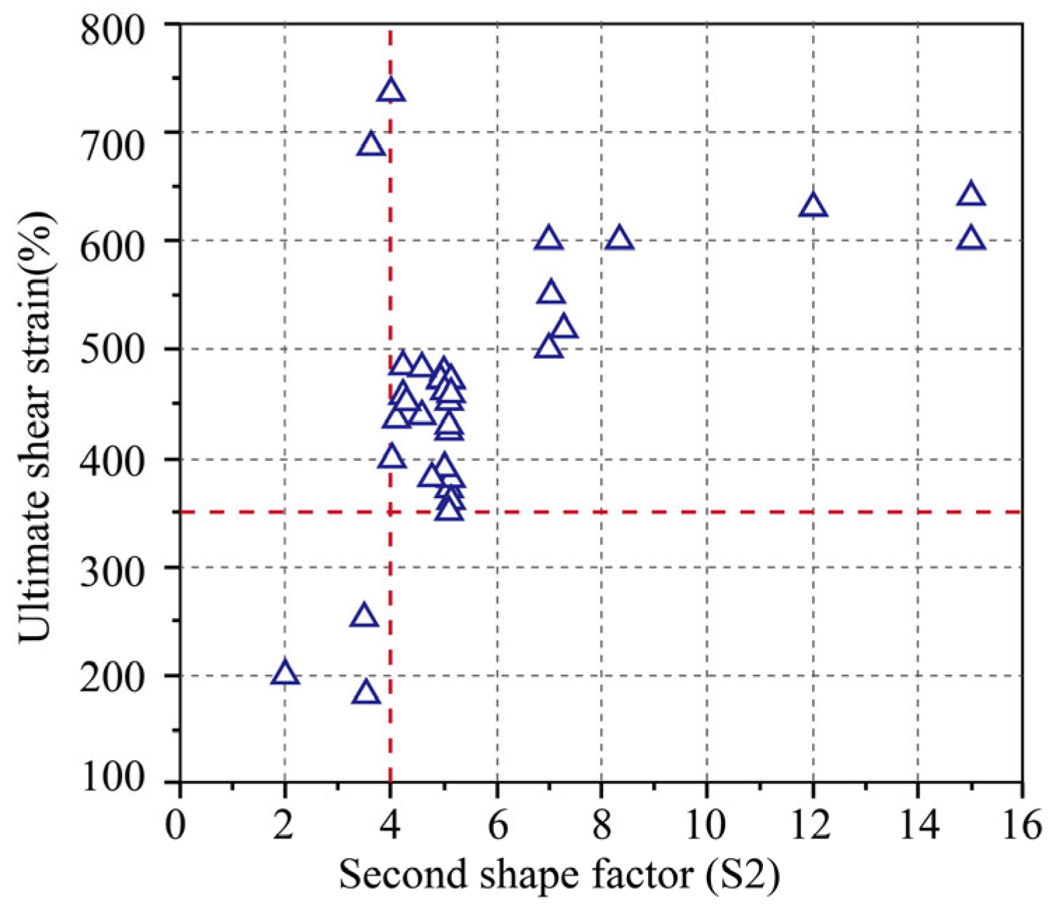
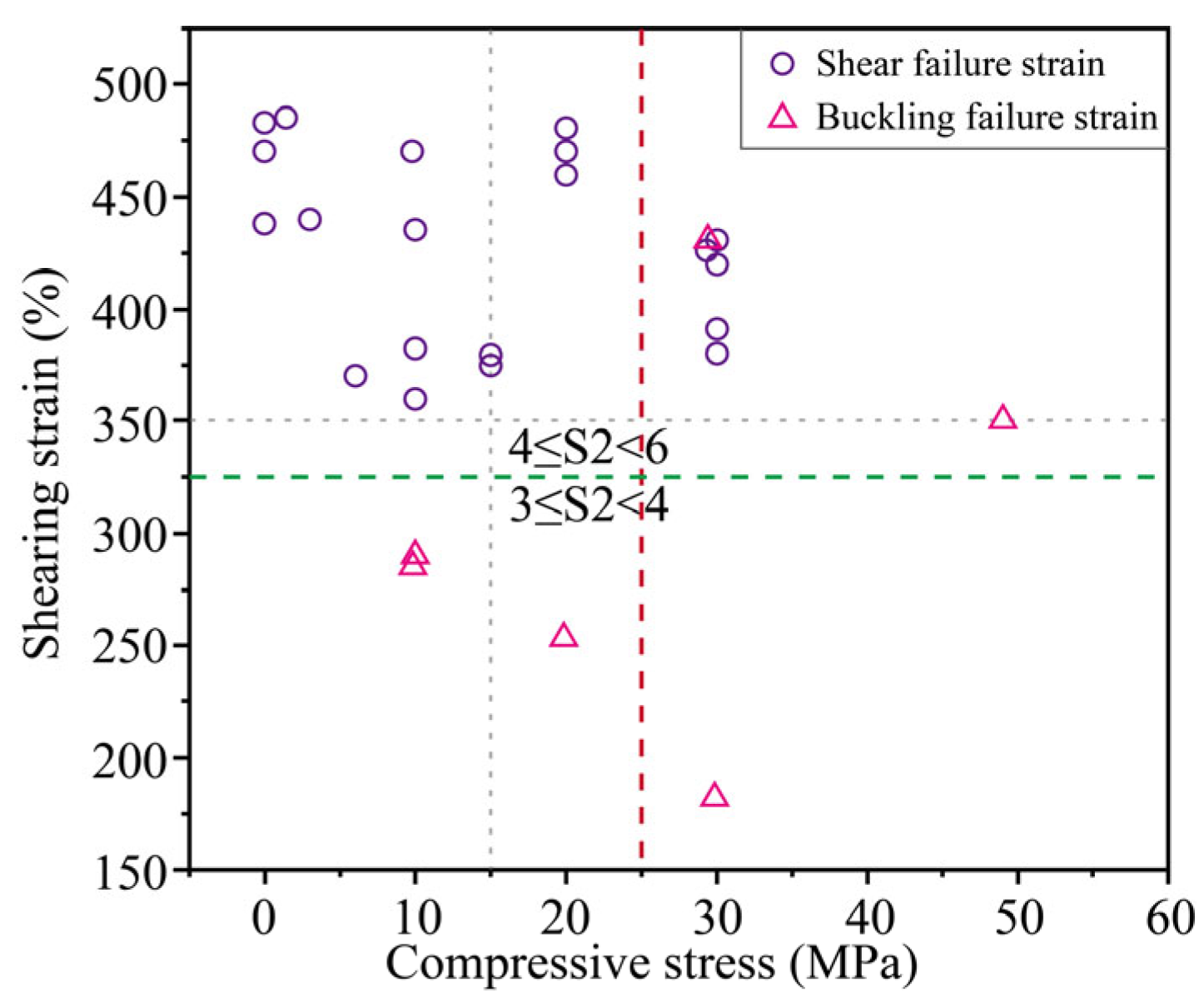
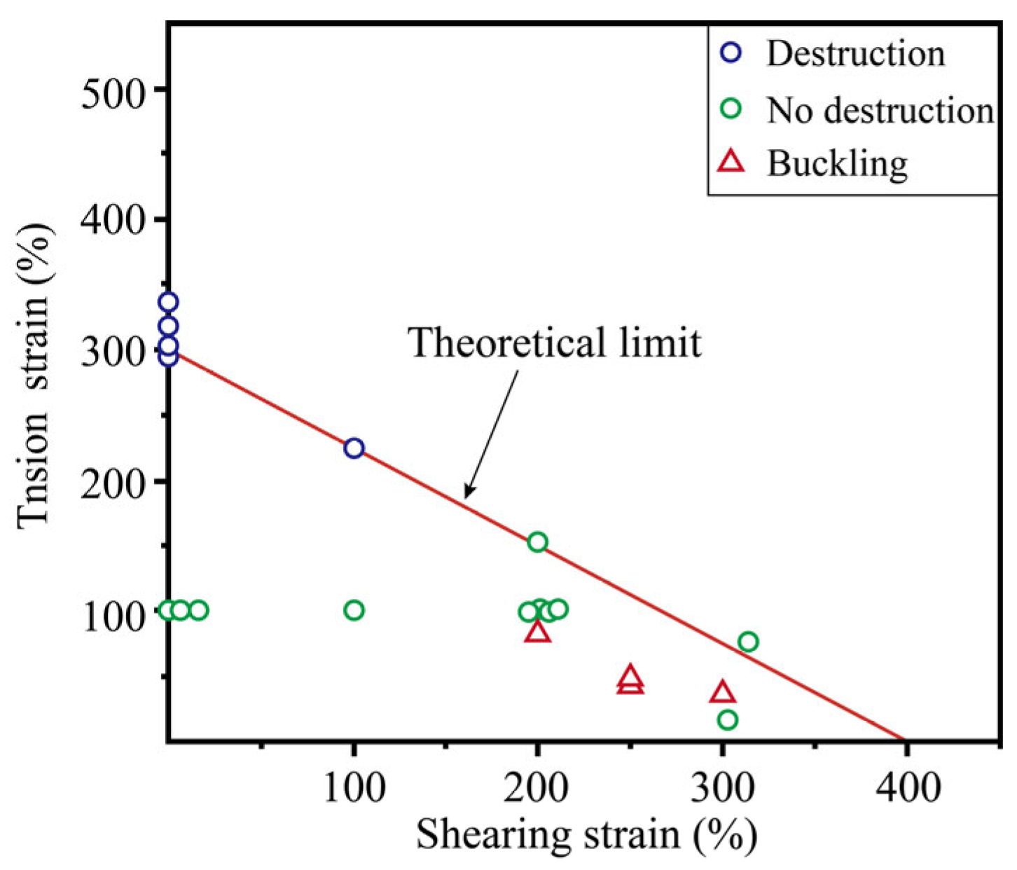
Based on the statistical analysis of experimental results from 102 rubber bearings, and in conjunction with relevant specifications, the thresholds for tensile-shear failure and compressive-shear failures have been established. Furthermore, the performance states of isolation bearings have been categorized into multiple levels. The integration with criteria for assessing the damage performance of concrete structures ensures a comprehensive and informative research process.

(3)

By comparing the calculations of the MDOF model with those of the finite element model, the computation speed of the MDOF model is reduced by 85%. Furthermore, the displacement time history and hysteresis curve of the top point of the isolation layer and the isolation layer itself essentially coincide with those of the finite element model, ensuring high computational accuracy. This indicates that rapid fragility analysis of isolated structures can be achieved using the MDOF model. It is important to note that the MDOF model does not include torsional degrees of freedom. This simplification was made to focus on translational behavior, and torsional effects will be addressed in future work.

(4)

The fragility analysis of the structure reveals that the fragility curves for both the upper structure and the isolation layer exhibit an upward trend, alternating in a staggered manner. It is advisable to comprehensively assess the damages to both the upper floors and isolation layers, using the severity of damage to the most affected floor as the overall damage level of the isolated structure. By strengthening the control of damage to the isolation layer, it is possible to enhance the overall seismic performance of the isolated structure.

It should be noted that the proposed method is currently applicable to base-isolated structures with regular mass and stiffness distribution. Torsional effects, axial–shear interaction in isolators, and detailed damping behavior are not considered in the present model. Additionally, the impact of pulse-like near-fault ground motions has not been included. The current study also does not account for the variability in structural and material properties. These simplifications were made to emphasize the efficiency of the proposed rapid assessment framework. Future research will incorporate these aspects to enhance the accuracy, robustness, and general applicability of the method.

References

1. Wang, X.; Qu, Z. Advantages of base isolation in reducing the reliability sensitivity to structural uncertainties of buildings. Eng. Struct. 2025, 323 Pt A, 119235. [Google Scholar] [CrossRef]
2. Shoma, K.; Michael, C.C. Probabilistic seismic performance assessment of seismically isolated buildings designed by the procedures of ASCE/SEI 7 and other enhanced criteria. Eng. Struct. 2019, 179, 566–582. [Google Scholar]
3. Ma, X.; Liu, Z.; Xiao, X. Seismic Fragility Analysis of a Multi-Tower Super High-Rise Building Under Near-Fault Ground Motions. J. Earthq. Eng. 2024, 28, 4301–4322. [Google Scholar] [CrossRef]
4. He, P.; Ma, Y.; Liu, C. Seismic resilience assessment of base-isolated structures with friction pendulum isolation bearings based on two-dimensional fragility. J. Build. Eng. 2025, 103, 112202. [Google Scholar] [CrossRef]
5. Zentner, I.; Gündel, M.; Bonfils, N. Fragility analysis methods: Review of existing approaches and application. Nucl. Eng. Des. 2017, 323, 245–258. [Google Scholar] [CrossRef]
6. Kennedy, R.P.; Ravindra, M.K. Seismic fragilities for nuclear power plant risk studies. Nucl. Eng. Des. 1984, 79, 47–68. [Google Scholar] [CrossRef]
7. Vamvatsikos, D.; Cornell, C.A. Incremental dynamic analysis. Earthq. Eng. Struct. Dyn. 2001, 31, 491–514. [Google Scholar] [CrossRef]
8. Li, S.Q.; Chen, Y.S.; Liu, H.B.; Carlo, D.G. Empirical seismic vulnerability assessment model of typical urban buildings. Bull. Earthq. Eng. 2023, 21, 2217–2257. [Google Scholar] [CrossRef]
9. Zhou, Y.; Jing, M.Y.; Pang, R.; Xu, B.; Jiang, F.; Yu, X. Stochastic dynamic response and seismic reliability analysis of nuclear power plant’s vertical retaining wall based on plastic failure. Structures 2021, 31, 513–539. [Google Scholar] [CrossRef]
10. Esteghamatim, Z.; Banazadehm, M.; Huang, Q.D. The effect of design drift limit on the seismic performance of RC dual high-rise buildings. Struct. Des. Tall Spec. Build. 2018, 27, 1464. [Google Scholar] [CrossRef]
11. Gautam, D.; Rupakhety, R. Empirical seismic vulnerability analysis of infrastructure systems in Nepal. Bull. Earthq. Eng. 2021, 19, 6113–6127. [Google Scholar] [CrossRef]
12. Lee, J.; Kong, J.; Kim, J. Seismic performance evaluation of steel diagrid buildings. Int. J. Steel Struct. 2018, 18, 1035–1047. [Google Scholar] [CrossRef]
13. Wu, F.; Luo, J.; Zheng, W.; Cai, C.; Dai, J.; Wen, Y.J.; Ji, Q.Y. Performance-based seismic fragility and residual seismic resistance study of a long-span suspension bridge. Adv. Civ. Eng. 2020, 2020, 8822955. [Google Scholar] [CrossRef]
14. Rakicevic, Z.; Bogdanovic, A.; Farsangi, E.N.; Sivandi-Pour, A. A hybrid seismic isolation system toward more resilient structures: Shaking table experiment and fragility analysis. J. Build. Eng. 2021, 38, 102194. [Google Scholar] [CrossRef]
15. Cardone, D.; Perrone, G.; Piesco, V. Developing collapse fragility curves for base-isolated buildings. Earthq. Eng. Struct. Dyn. 2019, 48, 78–102. [Google Scholar] [CrossRef]
16. Mangalathu, S.; Jeon, J.S.; DesRoches, R. Critical uncertainty parameters influencing seismic performance of bridges using Lasso regression. Earthq. Eng. Struct. Dyn. 2018, 47, 784–801. [Google Scholar] [CrossRef]
17. Sun, B.; Zhang, Y.; Huang, C. Machine Learning-Based Seismic Fragility Analysis of Large-Scale Steel Buckling Restrained Brace Frames. CMES-Comput. Model. Eng. Sci. 2020, 125, 755–776. [Google Scholar] [CrossRef]
18. Ruggieri, S.; Chatzidaki, A.; Vamvatsikos, D.; Uva, G. Reduced-order models for the seismic assessment of plan-irregular low-rise frame buildings. Earthq. Eng. Struct. Dyn. 2022, 51, 3327–3346. [Google Scholar] [CrossRef]
19. Folić, R.; Čokić, M. Fragility and vulnerability analysis of an RC building with the application of nonlinear analysis. Buildings 2021, 11, 390. [Google Scholar] [CrossRef]
20. Martins, L.; Silva, V. Development of a fragility and vulnerability model for global seismic risk analyses. Bull. Earthq. Eng. 2021, 19, 6719–6745. [Google Scholar] [CrossRef]
21. Zhao, D.; Wang, H.; Qian, H.; Jianming, L. Comparative vulnerability analysis of decomposed signal for the LRB base-isolated structure under pulse-like ground motions. J. Build. Eng. 2022, 59, 105106. [Google Scholar] [CrossRef]
22. Tajammolian, H.; Khoshnoudian, F.; Rad, A.R.; Loghman, V. Seismic fragility assessment of asymmetric structures support on TCFP bearing subjected to near-field earthquakes. Structures 2018, 13, 66–78. [Google Scholar] [CrossRef]
23. Sabet, B.; Talaeitaba, S.B. IDA analysis of regular and irregular seismically isolated structures in different stories and different seismic categories. Structures 2022, 43, 779–804. [Google Scholar] [CrossRef]
24. Xu, Z.D.; Zhang, T.; Huang, X.H. Dynamic analysis of three-directional vibration isolation and mitigation for long-span grid structure. J. Constr. Steel Res. 2023, 202, 107758. [Google Scholar] [CrossRef]
25. Delaviz, A.; Yaghmaei, S.S.; Souri, O. Seismic fragility and reliability of base-isolated structures with regard to superstructure ductility and isolator displacement considering degrading behavior. J. Earthq. Eng. 2024, 28, 3973–4002. [Google Scholar] [CrossRef]
26. Saha, S.K.; Matsagar, V.A.; Jain, A.K. Seismic fragility of base-isolated water storage tank sunder non-stationary earthquakes. Bull. Earthq. Eng. 2016, 14, 1153–1175. [Google Scholar] [CrossRef]
27. Liu, C.; Fang, D.; Yan, Z. Seismic fragility analysis of base isolated structure subjected to near-fault ground motions. Period. Polytech. Civ. Eng. 2021, 65, 768–783. [Google Scholar] [CrossRef]
28. Xiao, Y.; Ye, K.; He, W. An improved response surface method for fragility analysis of base-isolated structures considering the correlation of seismic demands on structural components. Bull. Earthq. Eng. 2020, 18, 4039–4059. [Google Scholar] [CrossRef]
29. Bhandari, M.; Bharti, S.D.; Shrimali, M.K.; Datta, T.K. Seismic fragility analysis of base-isolated building frames excited by near-and far-field earthquakes. J. Perform. Constr. Facil. 2019, 33, 04019029. [Google Scholar] [CrossRef]
30. Luo, C.; Wang, H.; Guo, X.X.; Wang, F.Y.; Tao, K.X.; Feng, H.P. Seismic fragility analysis of base-isolated structures based on response surface method. ASCE-ASME J. Risk Uncertain Eng. Syst. 2023, 9, 05023002. [Google Scholar] [CrossRef]
31. Takeda, T.; Sozen, M.A.; Nielsen, N.N. Reinforced concrete response to simulated earthquakes. J. Struct. Struct. Div. 1970, 96, 2557–2573. [Google Scholar] [CrossRef]
32. Yang, J.; Xia, Y.; Lei, X.; Limin, S. Hysteretic parameters identification of RC frame structure with Takeda model based on modified CKF method. Bull. Earthq. Eng. 2022, 20, 4673–4696. [Google Scholar] [CrossRef]
33. Li, Y.Z.; Cao, S.Y.; Xu, P.J.; Ni, X.Y. Experimental study on aseismic behavior of reinforced concrete columns with grade 600 MPa steel bars. Eng. Mech. 2018, 35, 181–189. [Google Scholar]
34. Lu, D.; Liu, W.G.; Qin, C.; He, W.F. Research on critical performance of domestic lead rubber bearings. Struct. Eng. 2016, 32, 146–151. [Google Scholar]
35. GB50011-2016; Code for Seismic Design of Buildings. Ministry of Housing and Urban-Rural Development: Beijing, China, 2016. (In Chinese)
36. Liu, W.G.; Yang, Q.R.; Zhou, F.L.; Feng, D.M. Nonlinear elastic extreme and buckling theory and experiment research on rubber isolators. Earthq. Eng. Eng. Vib. Chin. Ed. 2004, 24, 158–166. [Google Scholar]
37. AIJ. Recommendation for the Design of Seismically Isolated Buildings; Architectural Institute of Japan: Tokyo, Japan, 2013. [Google Scholar]
38. GB/T 51408-2021; Code for Seismic Isolation Design of Buildings. Ministry of Housing and Urban-Rural Development: Beijing, China, 2021. (In Chinese)
39. ASCE/SEI 41-17; Seismic Evaluation and Retrofit of Existing Buildings. American Society of Civil Engineers: Reston, VA, USA, 2017.
Figure 1. Single-degree-of-freedom system.
Buildings 15 02449 g001
Figure 2. Two-degree-of-freedom system.
Buildings 15 02449 g002
Figure 3. The ratio of the first-order natural vibration period to the isolation period.
Buildings 15 02449 g003
Figure 4. The ratio of the superstructure inter-story displacement to the lower mass displacement.
Buildings 15 02449 g004
Figure 5. Multi-degree-of-freedom isolation system.
Buildings 15 02449 g005
Figure 6. Modified Takeda model.
Buildings 15 02449 g006
Figure 7. Comparison of test curve and program calculation curve.
Buildings 15 02449 g007
Figure 8. Mechanical model of a lead–rubber bearing.
Buildings 15 02449 g008
Figure 9. Comparison of the hysteresis curve of the rubber bearing test and the Perform-3D software model curve.
Buildings 15 02449 g009
Figure 10. The relationship between bearing diameter and ultimate shear strain.
Buildings 15 02449 g010
Figure 11. The relationship between the second shape coefficient and the ultimate shear strain.
Buildings 15 02449 g011
Figure 12. The relationship between ts/tr and ultimate compressive stress.
Buildings 15 02449 g012
Figure 13. The relationship between bearing compressive stress and bearing damage failure mode.
Buildings 15 02449 g013
Figure 14. Theoretical curve of the tensile ultimate deformation of a rubber isolation bearing.
Buildings 15 02449 g014
Figure 15. Simple tensile failure test curve of isolation bearing.
Buildings 15 02449 g015
Figure 16. Failure limit curve of laminated rubber isolation bearing.
Buildings 15 02449 g016
Figure 17. Teaching building project effect diagram.
Buildings 15 02449 g017
Figure 18. Isolation bearing distribution design diagram.
Buildings 15 02449 g018
Figure 19. Seismic wave time history.
Buildings 15 02449 g019
Figure 20. Comparison of seismic response spectrum and standard response spectrum.
Buildings 15 02449 g020
Figure 21. Comparison of top displacement time history curves between the P3D and MDOF calculation programs.
Buildings 15 02449 g021
Figure 22. P3D and MDOF calculation program isolation layer hysteresis curve comparison.
Buildings 15 02449 g022
Figure 23. Comparison of interlayer displacement angle.
Buildings 15 02449 g023
Figure 24. Column plastic drift angle of the isolated structure under TH4-Y excitation.
Buildings 15 02449 g024
Figure 25. The performance state of frame columns on each floor under seven sets of envelope values of seismic conditions.
Buildings 15 02449 g025
Figure 26. Distribution of plastic displacement angles of beams on different floors.
Buildings 15 02449 g026
Figure 27. Damage degree of isolation bearing under rare earthquake.
Buildings 15 02449 g027
Figure 28. Damage in 0.62 g case.
Buildings 15 02449 g028
Figure 29. Damage in 0.72 g case.
Buildings 15 02449 g029
Figure 30. Damage in 0.84 g case.
Buildings 15 02449 g030
Figure 31. Large deformation hysteresis curve.
Buildings 15 02449 g031
Figure 32. Linear regression analysis: (a) superstructure demand parameters; (b) isolation layer demand parameters.
Buildings 15 02449 g032
Figure 33. Fragility curve of superstructure and isolation layer of isolation structure.
Buildings 15 02449 g033
Figure 34. Comparison of computation time between finite element software and MDOF program calculations.
Buildings 15 02449 g034