The Integrated ANN-NPRT-HUB Algorithm for Rail-Transit Networks of Smart Cities: A TOD Case Study in Chengdu

Abstract

Rail-transit hub classification in TOD refers to the categorization of transit stations based on their level of connectivity and ridership and the potential for development around them as part of a Transit-Oriented Development (TOD) strategy. TOD, as an essential concept in developing smart cities and public transportation accessibility, has attracted the focus of many policymakers. To this end, many research projects have been dedicated to classifying the rail-transit stations, although the necessity of integrated models for rail-transit hubs could have been mentioned in previous papers. Therefore, this parametric case study is directed to apply the Node–Place–Ridership–Time (NPRT) model to provide a logical classification model for Chengdu rail-transit hubs at the junctions of high-speed railway and subway stations. Multiple Linear Regression (MLR) provided a series of equations, including the effective parameters of the NPRT model. These equations were then verified by the Artificial Neural Network (ANN) to provide the effect of each node and place values on the integrated ridership of rail-transit hubs in different time periods. The results proved the consistent contribution of the integrated ANN-NPRT-HUB algorithm to the TOD concept for smart cities.

1. Introduction

A rail-transit hub is a transportation center where different modes of rail-based transportation intersect and connect, such as commuter trains, subways, light rail, and high-speed trains. These hubs are designed to facilitate the transfer of passengers and goods between different rail lines and modes of transportation and provide access to other forms of transportation, such as buses, taxis, and bicycles. Rail-transit hubs are typically located in urban areas and are often designed as multi-level structures with multiple platforms, tracks, and concourses. They may also include retail, dining, and other amenities to serve the needs of passengers and visitors. Examples of well-known rail-transit hubs include Grand Central Terminal in New York City, Gare du Nord in Paris, and Shinjuku Station in Tokyo. These hubs are critical transportation network components, providing a convenient and efficient way for people to move within and between cities and regions. Rail transit networks highlight the efficiency of public transportation in reducing air pollution and urban traffic loads, especially in developed cities such as Beijing, Shanghai, Chengdu, and New York [1,2,3].

A smart city is a concept that refers to the integration of technology and data-driven solutions to improve the quality of life, sustainability, and efficiency of urban areas. It uses advanced technologies, such as the Internet of Things (IoT), artificial intelligence (AI), and data analytics, to optimize various aspects of urban living, including transportation, energy, governance, infrastructure, and public services. The classification of railway transportation hubs using ANN, combined with a TOD approach, can help optimize urban transportation, enhance mobility services, improve real-time monitoring and management, and promote sustainable urban development. These elements collectively contribute to the development of smart cities by leveraging technology and data-driven solutions for a better urban living experience.

Critical stations, having the most significant impact on the rail transit network, are essential to smart cities’ transportation accessibility. These influential nodes could create critical areas, including other stations and rail-transit hubs, around themselves to facilitate the highly in-demand ridership destinations. Therefore, an accurate classification method for policymakers and city planners sounds vital to evaluate rail-transit hubs’ efficiency, especially in smart cities where people are encouraged daily to apply public transportation to reach their final destinations.

Transit-Oriented Development (TOD), as an applicable concept for developing smart cities and providing more access to public transportation, has attracted the attention of considerable researchers and municipal governments. TOD approaches supplement the analysis of the node function of the transit hubs, with a focus on the urban context often captured in the idea of place. To date, considerable research works have been conducted to propose station classification methods, such as Node–Place (NP) in 1999 [4], Node–Place–Ridership (NPR) in 2020 [5], and Node–Place–Ridership–Time (NPRT) in 2022 [6]. The NP model proposed by Bertolini provided a simple two-dimensional model for classifying stations with regards to their node and place values. According to this model, each station has five significant classes: Stress, Balance, Dependence, Unbalanced node, and unbalanced place.

Although NP was used for many years, ridership as a critical indicator did not receive any attention in this model. Therefore, Zhejing Cao et al. [5] proposed a new idea of considering ridership and creating a three-dimensional model of NPR. Their proposed model was comparably more accurate than the NP model, but the ridership was considered an independent value that could not prove the precise classification results that Ahad A. Pishro produced in 2022 [6]. Hence, we directed a research project on the effect of time as a critical indication of ridership and proposed a four-dimensional model of NPRT. A comprehensive analysis and comparison between NP, NPR, and NPRT models verified the logically accurate classification results for rail transit stations extracted from the NPRT model. In other words, the ridership is a dependent factor and varies during different time categories over weekdays and weekends [6]. This approach stream aims to enrich the initial NP model with key variables describing hubs and transit stations in their urban context, as an alternative to developing a complete transport model. Inspiration is also taken from the TOD literature with 3Ds and additional parameters [7,8,9]. Although all of the mentioned models have tried to provide classification methods, their focus was on stations and not hubs. An in-depth review of the existing literature showed the importance of having a precise hub rail transit classification method since the previous researchers have not achieved enough progress to propose a four-dimensional model for hubs in smart cities.

Many researchers tried to extend the classification models for a broader scale of rail transit networks by considering the high degree of centrality, betweenness, and topology property indexes while the ridership was neglected [10,11,12]. Zhang et al. [13] investigated the importance of transfer stations in the entire network. Wang et al. [14] applied the participation and z-score coefficient to determine the critical stations of the network in Dublin.

The classification of rail-transit hubs in TOD research is vital for effective planning, land use decision-making, understanding transit demand, promoting equity, and evaluating system performance. It provides a framework for analyzing and addressing the diverse needs of communities and facilitates the creation of sustainable, accessible, and efficient transportation systems. Classifying rail-transit hubs is crucial for understanding their characteristics and functionalities and guiding effective station design and infrastructure development. By categorizing hubs based on size, capacity, connectivity, and accessibility, planners and designers can make informed decisions regarding platform design, pedestrian flow management, parking facilities, and integration with other transportation modes. Additionally, hub classification is vital in determining land use patterns and enabling tailored land use policies and regulations that promote transit-supportive development, including mixed-use developments, higher density, and pedestrian-friendly environments. Understanding transit ridership and demand patterns is facilitated through station and hub classification, allowing researchers to analyze location, connectivity, proximity to residential and commercial areas, and parking availability, providing valuable insights for investment prioritization, resource allocation, and service planning. Moreover, hub classification helps identify disparities in transit access, facilitating efforts to address inequities through station improvements, equitable resource distribution, and targeted investments in underserved areas. Lastly, it supports performance evaluation by comparing metrics such as ridership, efficiency, service quality, and customer satisfaction across hub categories, allowing for benchmarking and targeted interventions to enhance the overall performance of rail transit systems.

This research considered the Chengdu rail transit network as the case study to investigate the NPRT algorithm for classifying the rail-transit hubs and study the correlations between the NPRT effective parameters. The Min–Max normalization method and the integrated NPRT values provided a reliable database for this study. Moreover, an Artificial Neural Network (ANN) was applied to predict and evaluate the results of our proposed NPRT-HUB model. The outcomes of this research aimed to provide new insight into the TOD concept with an exclusive focus on rail transit networks. These results can be implemented by municipal governments, city planners, and policymakers to adapt and improve the efficiency of their rail transit networks.

2. Methodology and Data Acquisition

2.1. Approach

This research is a case study on the Chengdu city rail transit network. Four hub district sizes were identified according to the results of questionnaires and statistical data collected from the riders, residents, and real estate. Each hub includes active rail transit stations which connect the whole district to the hub center. The hubs’ arrangement was assigned according to the counterclockwise direction starting from North. Regarding the statistical data and the questionnaire results, after several trials of integrating the stations’ data and applying the Min–Max normalization method, a 3000 m radius was set as the right active radius for the hubs.

Table 1 presents more details for our case study hubs. The Chengdu rail transit network, including four hubs, is shown in Figure 1.

Table 1. Chengdu rail-transit hubs.

Rail-Transit Hub	Active Radius (m)	Central Location
Hub 1	3000	North Railway Station
Hub 2	3000	West Railway Station
Hub 3	3000	South Railway Station
Hub 4	3000	East Railway Station

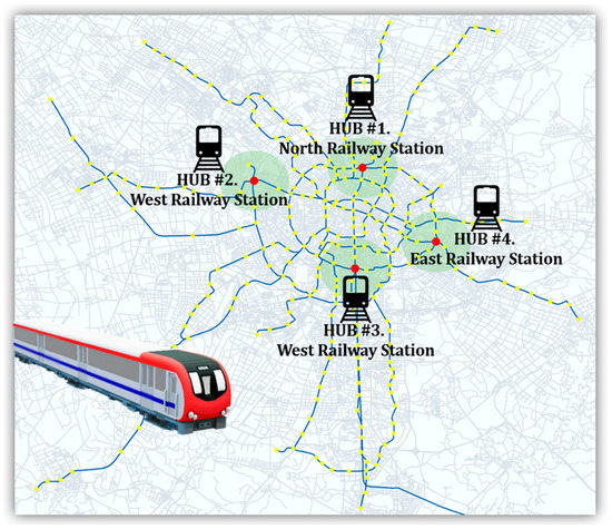
Figure 1. Chengdu rail-transit hubs.

We integrated the stations’ data and applied Min-Max normalization to provide a reliable database for each hub.

In this study, we employed a comprehensive methodology to analyze and classify rail-transit hubs using various data analysis techniques. First, we applied Min–Max Normalization to standardize the range of our data attributes, ensuring fair comparisons and preventing any attribute from dominating the classification process due to its scale. This normalization technique transformed the attribute values to a standard range between 0 and 1.

To determine the relative importance of attributes in the classification task, we utilized the Improved Entropy Weight (IEW) method. We assessed their diversity and randomness by calculating the entropy for each attribute. Lower entropy values indicated attributes with higher uniformity and specific information for classification. We assigned weights to the attributes based on these values, emphasizing those with lower entropy values. The attribute weights were then normalized to ensure meaningful comparisons and summing up to 1.

Next, we employed the Multiple Linear Regression (MLR) algorithms to build a classification model for rail-transit hubs. MLR allowed us to learn the linear relationship between input features (attributes) and the target variable (rail-transit hub classification). The attribute weights obtained from the IEW method were incorporated into the MLR model, giving higher importance to attributes with lower entropy during the training process.

To evaluate the performance of the MLR model, we utilized several metrics. Mean Squared Error (MSE) measured the average squared difference between the predicted and actual classification values, reflecting the model’s accuracy. $R^2$ (coefficient of determination) indicated the proportion of variance in the target variable that the MLR model could explain. Adjusted $R^2$ adjusted for the number of predictors, considering the model’s complexity and preventing overfitting.

We calculated the Variance Inflation Factor (VIF) to assess multicollinearity, which helped identify attributes with high intercorrelations that might impact the model’s stability and interpretability. Additionally, we employed statistical tests such as the F-Test and T-Test to evaluate the overall significance of the MLR model and the individual significance of the attribute coefficients, respectively. Finally, ANN was applied to predict and verify the results.

By integrating Min–Max Normalization, IEW, MLR, MSE, $R^2$, Adjusted $R^2$, VIF, F-Test, and T-test into our analysis pipeline, we gained insights into the classification of rail-transit hubs. These techniques allowed us to preprocess and normalize the data, determine attribute weights, build a classification model, assess its performance and significance, and address potential multicollinearity issues. This comprehensive approach provided a robust framework for analyzing and classifying rail-transit hubs.

This study advocates for a paradigm shift in the classification model by acknowledging and incorporating the time value. By completing three-dimensional models with time as a main dimension, the accuracy and precision of predictions can be significantly improved while also unraveling more profound correlations between various indicators. This approach aligns the classification model with the dynamic nature of real-world data, facilitating a more sophisticated understanding of evolving patterns and trends and ultimately leading to more reliable and insightful analyses.

Using mathematical concepts allows for a systematic and quantitative approach to the classification process. By leveraging mathematical models, factors such as connectivity, accessibility, and spatial patterns can be precisely analyzed and incorporated into the classification framework. This objective and data-driven methodology enhances the accuracy and reliability of the classification results. Moreover, the integration of ANN adds a powerful ML component to the classification process. ANN can effectively learn and recognize complex patterns and relationships within the data, enabling the identification of subtle nuances and hidden features that may not be readily apparent through traditional methods. This combination of mathematical concepts and ANN creates a sophisticated and advanced approach to classifying rail-transit hubs, facilitating a deeper understanding of their characteristics and aiding in the planning and development of transit-oriented communities. Therefore, using mathematical concepts and ANN in classifying rail-transit hubs within the context of TOD represents a cutting-edge and innovative approach that enhances decision-making and fosters sustainable urban development.

Figure 2 presents the research framework applied in this study.

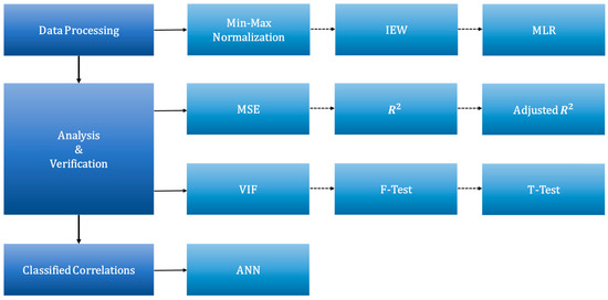
Figure 2. Research Framework.

2.2. NPRT Indicators

A list of NPR (node, place, and ridership) indicators are provided in Table 2. As mentioned before, the ridership value of each hub cannot be considered a constant or independent value since the number of people using the subway is different during working days and weekends. Moreover, on weekdays, three primary time categories lead to different ridership rates on the day. Therefore, we applied four time classes, T1 to T4, on weekdays and weekends to consider our hubs’ ridership value. Table 2 presents normalized integrated time classes applied in this research.

Table 2. Normalized Integrated Time class definition for the ANN-NPRT-HUB algorithm.

Time	Definition	Days	Hours	Max	Mean	Min
IT1	Inbound traffic during working hours	Monday to Friday	6:00–9:00	12,005.652	4643.215	540.652
IT2	Inbound traffic during off−hours	Monday to Friday	17:00–20:00	46,668.609	5735.578	561.478
IT3	Inbound traffic during the rest of the day	Monday to Friday	9:00–17:00/20:00–23:00	54,702.087	6720.584	782.913
IT4	Inbound traffic on two days of the weekend	Saturday and Sunday	6:00–23:00	51,955.625	5660.126	610.500
OT1	Passengers leaving the station during working hours	Monday to Friday	6:00–9:00	56,982.348	6788.879	581.348
OT2	Passengers leaving the station during off−hours	Monday to Friday	17:00–20:00	26,532.478	4930.341	349.609
OT3	Passengers leaving the station during the rest of the day	Monday to Friday	9:00–17:00/20:00–23:00	28,991.217	5501.752	411.522
OT4	Passengers leaving the station on both days of the weekend	Saturday and Sunday	6:00–23:00	55,496.875	5691.951	457.625

Table 3 fully describes the node and place value indicators, including relevant sub-branches. The node value has been divided into eight sections from $N1$ to $N8,$ represented by the principal concepts of TOD mentioned as sub-branches in this table. Moreover, $P1$ to $P9$ also provide nine sub-values of Place value.

Table 3. Node and Place Indicators.

Dimension	Sub − Branch	Indicator	Max	Mean	Min
Node Value	Station Facility	N1. Number of entrances and exits in each metro station (unit)	10.000	4.990	2.000
	Accessible Transits	N2. Number of metro stations that one station can reach within 20 min (unit)	88.000	59.311	19.000
		N3. Number of stations to CBD (Chunxi Road) (unit)	13.000	6.520	1.000
		N4. Number of stations to CBD (3rd Tianfu Street) (unit)	22.000	13.272	2.000
	Accessible Destinations	N5. Distance to CBD (Chunxi Road) (km)	17.006	7.388	0.862
		N6. Distance to CBD (3rd Tianfu Street) (km)	26.568	15.137	2.417
	Network Centrality	N7. Degree centrality	6.000	2.699	2.000
		N8. Closeness centrality (1/1000 km)	4767.649	3312.691	2731.193
Place Value	Design	P1. The average price of office land inside the 1000 m−radius catchment area (CNY/m2)	46,084.000	11,204.997	6600.000
	Density	P2. Number of offices within 1000 m (unit)	197.000	40.204	1.000
	Design	P3. The average price of commercial land inside the 1000 m−radius catchment area (CNY/m2)	34,310.900	22,414.351	15,553.143
	Density	P4. Number of shops within 1000 m (unit)	397.000	151.755	9.000
	Design	P5. The average price of residential land inside the 1000 m−radius catchment area (CNY/m2)	42,663.308	21,000.180	13,107.429
	Density	P6. Number of residences within 1000 m (unit)	552.000	163.699	8.000
	Diversity	P7. Number of public facilities (parks, cultural facilities, schools, hospitals) inside the 1000 m−radius catchment area (unit)	41.000	15.243	2.000
	Design	P8. Number of parking lots inside the 500 m−radius catchment area (unit)	132.000	28.748	0.000
		P9. Number of bus stops inside the 500 m−radius catchment area (unit)	26.000	8.592	1.000

Resources: SOSO (https://map.qq.com/ (accessed on 20 January 2023)), Amap (https://www.amap.com/ (accessed on 20 January 2023)), (https://www.chengdurail.com/index_en.html (accessed on 20 January 2023)), (https://www.chengdurail.com/index_en.html (accessed on 20 January 2023)), Anjuke (https://chengdu.anjuke.com/ (accessed on 20 January 2023)), Fang (https://cd.newhouse.fang.com/ (accessed on 20 January 2023)).

Normalized integrated node, place, and ridership values collected from all stations in each Hub area are presented in Table 4, Table 5 and Table 6, respectively.

Table 4. Normalized Integrated Node Indicators for each Hub.

Subway Station	N1	N2	N3	N4	N5	N6	N7	N8
Hub 1 (North Railway Station)	1.000	0.987	0.000	1.000	0.000	0.653	0.538	0.057
Hub 2 (West Railway Station)	0.759	0.000	1.000	0.891	1.000	1.000	0.000	1.000
Hub 3 (South Railway Station)	0.963	1.000	0.446	0.000	0.457	0.000	1.000	0.000
Hub 4 (East Railway Station)	0.000	0.221	0.185	0.663	0.297	0.573	0.668	0.954

Table 5. Normalized Integrated Place Indicators for each Hub.

Subway Station	P1	P2	P3	P4	P5	P6	P7	P8	P9
Hub 1 (North Railway Station)	0.056	1.000	1.000	1.000	0.000	1.000	1.000	1.000	0.000
Hub 2 (West Railway Station)	0.000	0.274	0.223	0.055	0.259	0.212	0.156	0.431	0.861
Hub 3 (South Railway Station)	0.899	0.947	0.894	0.115	1.000	0.433	0.566	0.718	1.000
Hub 4 (East Railway Station)	1.000	0.000	0.000	0.000	0.405	0.000	0.000	0.000	0.128

Table 6. Normalized Integrated Ridership for each Hub from IT1 to OT4.

Subway Station	IT1	IT2	IT3	IT4	OT1	OT2	OT3	OT4
Hub 1 (North Railway Station)	0.333	0.160	0.179	0.107	0.087	0.076	0.268	0.096
Hub 2 (West Railway Station)	0.877	0.000	0.000	0.180	0.041	0.523	0.000	0.123
Hub 3 (South Railway Station)	0.000	1.000	0.263	0.000	0.000	0.000	1.000	0.000
Hub 4 (East Railway Station)	1.000	0.493	1.000	1.000	1.000	1.000	0.036	1.000

2.3. Information Entropy Weighting (IEW)

Information Entropy Weighting (IEW) [15] was applied to compose the $N1-N8$ and $P1-P9$ value indexes into one integrated value of node and place, respectively. To this end, we could process the composed indicators to implement the database analysis started by the decision matrix presented in Equation (1). $m$ stations and $n$ node value indicators of each hub are consisted in $X$. $X_{pq}$ represents the value of indicator $q$ at station $p$. Equation (2) shows the decision matrix normalization:

$$X={\left\{X_{pq}\right\}}_{m\times n}$$

(1)

$$X_{pq}^{\prime }=\frac{X_{pq}-\min \left\{X_q\right\}}{\max \left\{X_q\right\}-\min \left\{X_q\right\}}$$

(2)

The proportion of station $p$ for indicator $q$ is calculated by Equation (3):

$$R_{pq}^{\prime }=\frac{X_{pq}^{\prime }}{{\sum }_{p=1}^m{X}_{pq}^{\prime }}$$

(3)

To compute the entropy value $e_q$ of indicator $q$, we can apply Equation (4):

$$e_q=-\frac{1}{\ln m}\times {\displaystyle \sum }_{p=1}^m{R}_{pq}^{\prime }.\ln R_{pq}^{\prime }$$

(4)

If $R_{pq}^{\prime }=0$, then $\ln R_{pq}^{\prime }=0.$

The imbalance coefficient is shown in Equation (5):

$$g_q=1-e_q$$

(5)

Equation (10) provides the weight of indicator $q$ indicated by $W_q$. The result of Equation (6) is used in Equation (7) to compose the $N_p$ (node value index) for station $p$.

$$W_q=\frac{g_q}{{\sum }_{q=1}^n{g}_q}$$

(6)

$$N_p={\displaystyle \sum }_{q=1}^n{W}_q\times X_{pq}^{\prime }$$

(7)

To normalize the node value index in [0, 1], we apply Equation (8), in which $N$ denotes the index in the array of node values, $m$ indicates the number of stations, and $p$ is the target station:

$$N_p^{\prime }=\frac{N_p-\min \left\{N\right\}}{\max \left\{N\right\}-\min \left\{N\right\}}$$

(8)

2.4. Multiple Linear Regression (MLR)

In this study, we applied Multiple Linear Regression (MLR) to investigate the relationships between the effective parameters (factor variable and multiple variables) on our TOD models and equations.

Regarding the linear Equation (9), $a_1$ and $a_2$ can be determined by applying linear regression of multiple variables using machine learning techniques.

$$u=a_1{x}_1+a_2{x}_2$$

(9)

The MLR equations are a regression analysis applying the least-square function to model the argument relationships. This function provides a linear combination of one or more effective parameters, known as regression coefficients [16].

The corresponding model for our n-dimensional feature sample data using linear regression is presented in Equation (10):

$$h_{\theta }\left(x_1,x_2,\cdots ,x_n\right)={\theta }_0+{\theta }_1{x}_1+\cdots +{\theta }_n{x}_n$$

(10)

A simplified equation considering $x_0=1$ would be:

$$h_{\theta }\left(x_0,x_1,x_2,\cdots ,x_n\right)={\displaystyle \sum }_{i=0}^n{\theta }_i{x}_i$$

(11)

The matrix form provides a more concise understanding of the above equations:

$$h_{\theta }\left(X\right)=X\theta ,$$

(12)

where

$$\theta =\left[\begin{array}{c}{\theta }_0\\ {\theta }_1\\ \begin{array}{c}⋮\\ {\theta }_n\end{array}\end{array}\right],x=\left[\begin{array}{c}{x}_0\\ x_1\\ \begin{array}{c}⋮\\ x_n\end{array}\end{array}\right],Y=\left[\begin{array}{c}{y}_0\\ y_1\\ \begin{array}{c}⋮\\ y_n\end{array}\end{array}\right],X=\left[\begin{array}{ccc}{x}_{01}& \cdots & x_{0n}\\ ⋮& \ddots & ⋮\\ x_{m1}& \cdots & x_{mn}\end{array}\right]$$

(13)

In Equation (13) $m$ denotes the number of samples and $n$ presents the number of sample features. We use the Mean Square Error (MSE) as the loss function for our linear regression model. The algebraic equation and the matrix form of the loss function are presented in Equations (14) and (15), respectively.

$$J\left({\theta }_0,{\theta }_1,{\theta }_2,\cdots ,{\theta }_n\right)={\displaystyle \sum }_{i=0}^m{\left(h_{\theta }\left(x_0,x_1,x_2,\cdots ,x_n\right)-y_i\right)}^2$$

(14)

$$J\left(\theta \right)={\left(X\theta -Y\right)}^T\left(X\theta -Y\right)$$

(15)

Applying Equations (16) and (17) and parameter estimation of the MLR model leads to minimizing of the loss function.

$$\frac{\partial J\left(\theta \right)}{\partial \theta }=2X^{T}X\theta -2X^{T}Y$$

(16)

Then,

$$\theta ={\left(X^{T}X\right)}^{-1}{X}^{T}Y$$

(17)

Thus, the following multilinear regression model is achieved.

$$f\left(x\right)=x^T{\left(X^{T}X\right)}^{-1}{X}^{T}Y$$

(18)

3. Machine Learning Application in TOD

An Artificial Neural Network (ANN), as an application of Machine Learning (ML), is widely used to predict outcomes, classify the results, and check the accuracy of research achievements. Seven main steps create the primary process of ANN applications: importing the data, cleaning the data, splitting the data into training/test sets, model creation, model training, predictions, and model evaluation and improvement.

The ANN structure is created by three main layers, shown in Figure 3. For simplicity, the activation function is not shown in the figure; therefore, we use the same one between two adjacent layers.

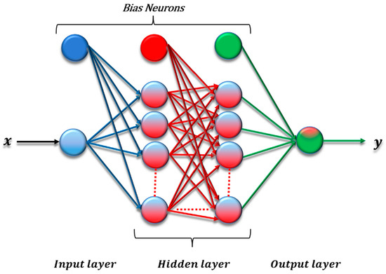
Figure 3. ANN structure [17].

The ANN structure directs the input to output in one-way information processing. After receiving the input data by the ANN, the error value is calculated. Each layer contains groups of neurons that have their importance determined by assigned weight. The backpropagation algorithm leads to learning and solving errors based on the data of the input and output layers. Mean Square Error (MSE) provides a valuable loss function for regression problems to predetermine the logical minimum error [16,17,18].

$$MSE\left(y, y^{\prime }\right)=\frac{{\sum }_{i=1}^n{\left(y_i-y_i^{\prime }\right)}^2}{n}$$

(19)

In this research, the neurons’ activation function ($f$) supports the Rectified Linear Unit $\left(ReLU\right)$ function, as shown in Figure 4.

$$ReLU\left(x\right)=\{\begin{array}{c}x if x>0\\ 0 if x\le 0\end{array}$$

(20)

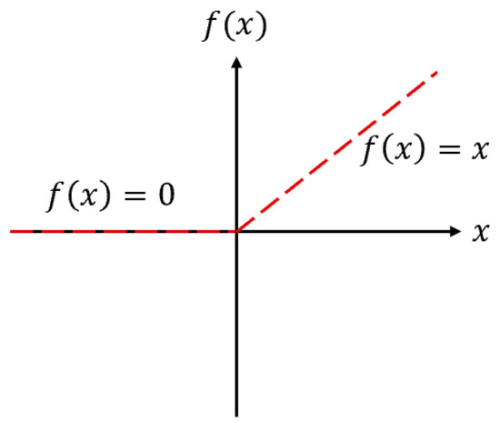
Figure 4. The neurons’ activation function ($f$) [17].

Based on the existing applications of deep learning methods [19,20,21,22,23,24], this study applied the MSE loss function, shown in Figure 5. Moreover, adaptive moment estimation (ADAM) was used to optimize the convergence and enhance the model accuracy.

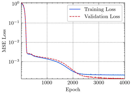
Figure 5. Loss function, MSE.

Model Evaluation Method

As mentioned before, to verify the Multiple Linear regression (MLR) equations’ accuracies of fit in the regression method, we used the Mean Square Error (MSE), presented in Equation (21).

$$MSE=\frac{1}{n}{\displaystyle \sum }_{i=1}^n{\left(y_i-\widehat{f}\left(x_i\right)\right)}^2$$

(21)

The Multiple Determination Coefficients $\left(R^2\right)$, a valuable indicator to evaluate the convergence of MLR equations, reflects the proportions described by the estimated regression equations in the variance of the factor variable $y$, calculated as the proportion of progression squares to the sum of total squares [25].

Regarding Equations (22)–(24), ${\widehat{y}}_i$ shows the model forecast value, $\overline{y}$ stands for the average of $y$, $SSR$ indicates the Regression Sum of Squares, $SSE$ represents the Error Sum of Squares, and $SST$ denotes the Total Sum of Squares [16,17,25].

$$SSR={\displaystyle \sum }_{i=1}^m{\left({\widehat{y}}_i-\overline{y}\right)}^2$$

(22)

$$SSE={\displaystyle \sum }_{i=1}^m{\left(y_i-\overline{y}\right)}^2$$

(23)

$$R^2-\frac{SSR}{SST}=1-\frac{SSE}{SST}$$

(24)

4. Results and Discussion

4.1. The NPRT Variables’ Correlations

We applied Python as a high-level programming language for creating our ANN-NPRT-HUB algorithm and investigated the correlations between independent values (node and place) and dependent values (integrated ridership-time). Using Python’s pandas and numpy libraries, the correlations between the positive or negative variables were obtained and presented in Table 7. A positive correlation is a statistical measure that signifies a simultaneous increase in one variable as the other variable also experiences an increase. This phenomenon implies that the two variables exhibit a coherent behavior, moving in the same direction. Conversely, a negative correlation denotes an inverse relationship, wherein an increase in one variable corresponds to a decrease in the other variable. This indicates a tendency for the variables to move in opposite directions. A correlation coefficient is employed to ascertain the magnitude of the correlation, offering a numerical representation of the relationship between the variables. The correlation coefficient ranges from −1 to 1, providing valuable insights into the strength and direction of the correlation. A correlation coefficient close to 1 or −1 implies a robust correlation, with the variables exhibiting a highly consistent pattern of behavior. In contrast, a coefficient closer to 0 suggests a weaker correlation, indicating that the variables have less synchrony in their variations.

Table 7. The correlations between dependent and independent values.

Independent Values	Dependent Values
	IT1	IT2	IT3	IT4	OT1	OT2	OT3	OT4
N1	−0.771334	−0.00302	−0.89232	−0.98724	−0.96816	−0.95286	0.529008	−0.98187
N2	−0.920694	0.51648	−0.19789	−0.53933	−0.42357	−0.81764	0.765575	−0.49288
N3	0.262923	−0.2372	−0.49709	−0.26712	−0.37334	0.092877	−0.13028	−0.31042
N4	0.581252	−0.95709	−0.13298	0.176322	0.102728	0.296284	−0.86524	0.143892
N5	0.347413	−0.21838	−0.38831	−0.15149	−0.2593	0.20443	−0.178	−0.19509
N6	0.750428	−0.96956	−0.20556	0.187105	0.072138	0.445079	−0.91666	0.13838
N7	−0.635475	0.913791	0.422403	0.02761	0.154792	−0.30006	0.774317	0.081373
N8	0.958216	−0.48371	0.330308	0.654078	0.548117	0.89137	−0.79245	0.611863
P1	−0.081878	0.837763	0.767937	0.513484	0.589733	0.300946	0.419866	0.547957
P2	−0.937089	0.28764	−0.56859	−0.81855	−0.73908	−0.97225	0.709613	−0.7879
P3	−0.925206	0.274289	−0.53634	−0.78837	−0.70582	−0.95717	0.686738	−0.7565
P4	−0.397904	−0.33189	−0.33953	−0.39838	−0.35263	−0.55255	0.002391	−0.38259
P5	−0.481973	0.9115	0.121717	−0.1438	−0.08788	−0.21237	0.798931	−0.11843
P6	−0.644239	−0.15213	−0.52795	−0.64919	−0.594	−0.78908	0.274455	−0.6295
P7	−0.763744	0.024199	−0.49458	−0.67969	−0.60735	−0.85408	0.435999	−0.65261
P8	−0.793568	−0.01781	−0.72169	−0.8638	−0.81557	−0.94264	0.479526	−0.84677
P9	−0.303243	0.359447	−0.48772	−0.51308	−0.54549	−0.30907	0.504687	−0.52547

Using the correlations between the values provided in Table 7, we can adjust and improve the efficiency of each rail-transit hub by increasing or decreasing the corresponding value(s). The correlation between variables can provide valuable insights into optimizing the efficiency of rail-transit hubs. By focusing on these critical factors, improvements can be targeted where they have the most significant impact.

4.2. MLR Equations for the ANN-NPRT-HUB Model

This research applied Multiple Linear Regression (MLR) to extract eight regression equations for the proposed ANN-NPRT-HUB model. A comprehensive form for the MLR equations is presented in Equation (25). This equation is made of three main terms. $\alpha$ indicates the intercept, while $\beta$ and $\gamma$ represent the coefficients of node and place values, respectively. To determine the three parameters of $\alpha$, $\beta$, and $\gamma$, from the sklearn.linear_model of Python, we imported the LinearRegression function.

$$Ridership=\alpha +{\displaystyle \sum }_{i=1}^8{\beta }_i{N}_i+{\displaystyle \sum }_{j=1}^9{\gamma }_j{P}_j$$

(25)

Appendix A provides a list of constants and variable coefficients for the dependent variable of IT1 to OT4. The complete results of our MLR models are presented in Table 8.

Table 8. MLR models results.

	IT1		IT2		IT3		IT4		OT1		OT2		OT3		OT4
Ad.R2	0.3		0.467		0.245		0.206		0.252		0.227		0.589		0.234
	CV	p	CV	p	CV	p	CV	p	CV	p	CV	p	CV	p	CV	p
Constant	−4595.88	0.723	12,022.14	0.643	181,04.91	0.633	11,838.94	0.715	8425.112	0.811	−2767.62	0.877	−2767.62	0.84	5025.627	0.877
N1	−25.376	0.889	−657.282 *	0.074	−1318.949 **	0.015	−964.227 **	0.036	−1083.452 **	0.03	−346.841	0.169	−346.841	0.143	−943.496 **	0.041
N2	7.483	0.915	−48.441	0.728	−106.723	0.6	−89.607	0.607	−67.367	0.721	−8.61	0.928	−8.61	0.966	−58.054	0.739
N3	561.364	0.214	630.5	0.483	500.433	0.703	393.954	0.726	431.01	0.724	612.772	0.323	612.772	0.403	368.891	0.743
N4	−449.041 **	0.025	−815.953 **	0.04	−942.555	0.103	−854.403 *	0.084	−846.086	0.115	−654.006 **	0.017	−654.006 *	0.078	−770.442	0.12
N5	−867.804 **	0.031	−1129.19	0.156	−1366.88	0.239	−1196	0.228	−1289.4	0.231	−1075.195 *	0.051	−1075.195	0.192	−1142.52	0.25
N6	234.298	0.161	570.856 *	0.088	850.038 *	0.083	761.852 *	0.069	781.668 *	0.085	443.716 *	0.055	443.716	0.219	714.178 *	0.089
N7	326.503	0.438	2316.741 ***	0.007	3954.057 ***	0.002	3022.925 ***	0.005	3267.77 ***	0.005	1137.145 *	0.052	1137.145 ***	0.006	2934.299 ***	0.006
N8	3.8	0.15	−0.784	0.881	−2.142	0.78	−0.798	0.903	−0.252	0.972	2.893	0.423	2.893	0.934	0.17	0.979
P1	0.004	0.948	−0.03	0.808	−0.047	0.796	−0.044	0.777	−0.061	0.714	−0.007	0.936	−0.007	0.68	−0.055	0.724
P2	−33.321 ***	0.002	96.926 ***	0.001	63.024 **	0.043	39.064	0.14	53.189 *	0.066	−6.939	0.633	−6.939 ***	0.001	45.053 *	0.091
P3	0.028	0.722	0.03	0.846	0.137	0.546	0.144	0.457	0.165	0.433	0.093	0.383	0.093	0.903	0.165	0.396
P4	16.891 **	0.026	12.614	0.4	18.805	0.391	27.532	0.143	26.859	0.188	23.934 **	0.022	23.934 **	0.882	28.477	0.131
P5	−0.111 *	0.089	0.057	0.66	0.031	0.869	0.03	0.853	0.054	0.76	−0.052	0.561	−0.052	0.696	0.057	0.726
P6	−2.658	0.587	−7.99	0.414	−10.479	0.463	−8.525	0.485	−10.502	0.428	−3.731	0.579	−3.731	0.379	−9.079	0.458
P7	−31.787	0.496	−183.022*	0.052	−151.554	0.267	−172.084	0.141	−177.163	0.163	−95.857	0.137	−95.857	0.232	−173.106	0.14
P8	22.276	0.287	−7.219	0.862	15.054	0.805	3.561	0.945	12.022	0.832	10.351	0.718	10.351	0.925	2.635	0.96
P9	157.088 **	0.03	−52.297	0.714	−73.514	0.725	−85.692	0.631	−50.335	0.795	81.313	0.409	81.313	0.7	−72.751	0.684

If p < 0.01 ⇒ ***; p < 0.05 ⇒ **; p < 0.1 ⇒ *, CV: Coefficient of Variation.

The Ad.R² indicates how well the model fits the data, with a value of 1 indicating a perfect fit. Generally, a value of Ad.R² greater than 0.2 is considered acceptable for the fitted model. In statistical analysis, the significance level of a result is typically represented by the p value, where a smaller p value corresponds to a more substantial effect of the independent variable on the dependent variable. The coefficient of variation (CV) indicates the impact of an independent variable on a dependent variable. A higher CV value indicates a more substantial influence of the independent variable on the dependent variable. And a negative CV implies a negative correlation between the independent and dependent variables.

Applying the constant and coefficient values from Table 8 to Equation (25), we can construct a series of eight MLR equations for the rail-transit hubs provided in Table 9.

Table 9. Extracted MLR Equations.

General MLR Equation (25)	Extracted MLR Equations from Table 8
$Ridership=\alpha +{\displaystyle {\displaystyle \sum }_{i=1}^8}{\beta }_i{N}_i+{\displaystyle {\displaystyle \sum }_{j=1}^9}{\gamma }_j{P}_j$	$\begin{array}{cc}\hfill I{T}_1=-4595.878& -25.376N_1+7.483N_2+561.364N_3-449.041N_4-867.804N_5+234.298N_6\hfill \\ \hfill & +326.503N_7+3.8N_8+0.004P_1-33.321P_2+0.028P_3+16.891P_4-0.111P_5\hfill \\ \hfill & -2.658P_6-31.787P_7+22.276P_8+157.088P_9\hfill \end{array}$
	$\begin{array}{cc}\hfill I{T}_2=12022.143& -657.282N_1-48.441N_2+630.5N_3-815.953N_4-1129.194N_5+570.856N_6\hfill \\ \hfill & +2316.741N_7-0.784N_8-0.03P_1+96.926P_2+0.03P_3+12.614P_4+0.057P_5\hfill \\ \hfill & -7.99P_6-183.022P_7-7.219P_8-52.297P_9\hfill \end{array}$
	$\begin{array}{cc}\hfill I{T}_3=18104.908& -1318.949N_1-106.723N_2+500.433N_3-942.555N_4-1366.881N_5+850.038N_6\hfill \\ \hfill & +3954.057N_7-2.142N_8-0.047P_1+63.024P_2+0.137P_3+18.805P_4+0.031P_5\hfill \\ \hfill & -10.479P_6-151.554P_7+15.054P_8-73.514P_9\hfill \end{array}$
	$\begin{array}{cc}\hfill I{T}_4=11838.943& -964.227N_1-89.607N_2+393.954N_3-854.403N_4-1196.002N_5+761.852N_6\hfill \\ \hfill & +3022.925N_7-0.798N_8-0.044P_1+39.064P_2+0.144P_3+27.532P_4+0.03P_5\hfill \\ \hfill & -8.525P_6-172.084P_7+3.561P_8-85.692P_9\hfill \end{array}$
	$\begin{array}{cc}\hfill O{T}_1=8425.112& -1083.452N_1-67.367N_2+431.01N_3-846.086N_4-1289.399N_5+781.668N_6\hfill \\ \hfill & +3267.77N_7-0.252N_8-0.061P_1+53.189P_2+0.165P_3+26.859P_4+0.054P_5\hfill \\ \hfill & -10.502P_6-177.163P_7+12.022P_8-50.335P_9\hfill \end{array}$
	$\begin{array}{cc}\hfill O{T}_2=-2767.615& -346.841N_1-8.61N_2+612.772N_3-654.006N_4-1075.195N_5+443.716N_6\hfill \\ \hfill & +1137.145N_7+2.893N_8-0.007P_1-6.939P_2+0.093P_3+23.934P_4-0.052P_5\hfill \\ \hfill & -3.731P_6-95.857P_7+10.351P_8+81.313P_9\hfill \end{array}$
	$\begin{array}{cc}\hfill O{T}_3=-2767.615& -346.841N_1-8.61N_2+612.772N_3-654.006N_4-1075.195N_5+443.716N_6\hfill \\ \hfill & +1137.145N_7+2.893N_8-0.007P_1-6.939P_2+0.093P_3+23.934P_4-0.052P_5\hfill \\ \hfill & -3.731P_6-95.857P_7+10.351P_8+81.313P_9\hfill \end{array}$
	$\begin{array}{cc}\hfill O{T}_4=5025.627& -943.496N_1-58.054N_2+368.891N_3-770.442N_4-1142.524N_5+714.178N_6\hfill \\ \hfill & +2934.299N_7+0.17N_8-0.055P_1+45.053P_2+0.165P_3+28.477P_4+0.057P_5\hfill \\ \hfill & -9.079P_6-173.106P_7+2.635P_8-72.751P_9\hfill \end{array}$

Multiple Linear Regression (MLR) equations can be highly beneficial for analyzing ridership in rail-transit hubs. MLR models provide a statistical framework for understanding the relationships between multiple independent variables and the dependent variable of ridership. By considering various factors influencing ridership, MLR equations offer valuable insights into understanding and forecasting the demand for rail-transit services.

4.3. Classification Results

Applying the MLR equations of Table 9 and the NP (Node, Place) values, we can achieve the actual ridership values of the NPRT model for rail-transit hubs. Moreover, we used the ANN to predict the NPRT model results presented in this research. Table 10 shows a list of predicted values provided by the ANN and the MLR equations’ actual results. In this table, p denotes the predicted value.

Table 10. Predicted and actual results.

Model	HUB 1	HUB 2	HUB 3	HUB 4
P.IT1	4553.709	7765.223	5191.758	5850.328
IT1	4310.488	10,068.957	5140.873	5622.964
P.IT2	4429.563	7269.329	7246.624	4512.556
IT2	3406.512	8087.725	6822.873	5015.938
P.IT3	6150.541	9040.156	7015.845	6246.506
IT3	4647.051	10,010.928	6434.328	7915.960
P.IT4	5542.270	8464.807	5749.719	5772.651
IT4	4147.919	9412.0	5058.965	6851.5
P.OT1	6544.339	9521.689	6955.400	6470.205
OT1	5012.225	10,658.768	6402.264	7585.407
P.OT2	4708.928	8213.316	5364.432	5646.256
OT2	3970.437	10,121.782	5294.794	5663.470
P.OT3	4708.928	8213.316	5364.432	5646.256
OT3	3279.386	7510.681	6796.430	3806.182
P.OT4	5596.776	8303.321	5695.017	5520.744
OT4	4165.272	9155.417	5093.886	6416.920

The ANN-predicted ridership for individual rail-transit hubs holds significant importance in various technical aspects. It primarily enables effective demand forecasting, capacity planning, resource allocation, service optimization, revenue estimation, and decision-making. Leveraging the capabilities of ANN models empowers transit authorities to make well-informed decisions to enhance operational efficiency, improve the passenger experience, and ensure the sustainable growth and development of rail transit systems.

In Table 10, the predicted ridership by the ANN is based on the underlying patterns and associations discovered during the model training. By leveraging the power of the ANN, which excels in capturing intricate relationships in complex datasets, transit authorities gain insights into the anticipated demand for each rail-transit hub.

Figure 6 illustrates a comparison between the actual NPRT-HUB results created by MLR equations and the predicted ones by the ANN. As mentioned before, the predicted classes can be distinguished by the letter p before the name of the class. This figure shows that the ANN could logically predict the NPRT model ridership values. For example, the ANN predicted that the class $I{T}_1$ covers 19% of the ridership of HUB#1 (North Railway Station), while the actual MLR value is 17%. This logical prediction comes true while looking at the other hubs’ classes, such as $PO{T}_2$ and $O{T}_2$ for HUB#4 (East Railway Station), with values of 24% and 23%, respectively. Therefore, applying the ANN in classifying and assessing the efficiency of rail-transit hubs could bring new insight into TOD.

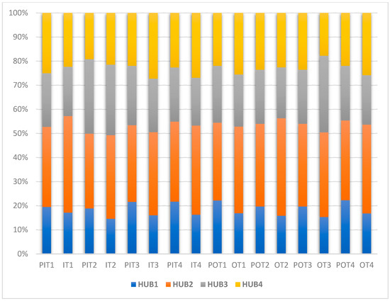
Figure 6. Comparison between the predicted and actual NPRT-HUB results.

ANNs can be helpful for city planners in assessing the rail-transit hubs because they can assist in identifying significant patterns and relationships within large and complex datasets. In the case of rail-transit hubs, ANNs can be used to analyze data on passenger flows, station usage, train schedules, and other factors that affect the efficiency and effectiveness of a hub. Using ANNs, city planners can create predictive models to help them make informed decisions about optimizing a rail-transit hub’s performance. For example, ANNs can forecast passenger demand at different times of the day or during special events, allowing transit planners to adjust train schedules and allocate resources accordingly. ANNs can also identify patterns in passenger behavior, such as how they move through a station or which routes they tend to take, which can inform decisions about station design and layout. In addition to these practical applications, ANNs can also be used to test hypothetical scenarios and predict the potential impact of different planning decisions. For example, planners can use ANNs to simulate the effects of adding new train lines or changing the location of a station, helping them make informed decisions that will benefit both passengers and the city as a whole.

Rail-transit hub classification empowers city planners and policymakers to optimize network efficiency. It guides network optimization, service planning, infrastructure development, land use decisions, and policy formulation. By using the results of hub classification, cities can create more efficient and sustainable rail transit networks that cater to the diverse needs of their residents and visitors. Classification helps identify key hub types, such as significant transfer or high-demand ones, which require specific infrastructure and operational considerations. Planners can strategically allocate resources, prioritize investments, and optimize service frequencies to ensure efficient connectivity and minimize delays and congestion. For example, a city may identify a particular hub as a central transfer point between multiple rail lines and allocate additional platform space and staffing to facilitate smooth transfers and reduce overcrowding. Hub classification assists in determining service patterns and frequencies based on hub types. Planners can allocate more frequent service to high-demand hubs, ensuring efficient transportation access for a larger population.

Conversely, lower-demand hubs may receive less frequent service, optimizing resource utilization. For instance, a city may identify specific hubs as high-demand destinations due to their proximity to employment centers or popular tourist attractions. Higher service frequencies can be scheduled during peak hours to accommodate commuter and tourist travel.

By understanding the characteristics of different hub types, city planners can make informed decisions about infrastructure development and station design. For example, if a hub is classified as a major transfer point, planners can allocate sufficient space for platform-to-platform transfers, install clear wayfinding signage, and ensure adequate accessibility features. This promotes smooth passenger flow and minimizes bottlenecks, contributing to overall network efficiency. Rail-transit hub classification informs land use and development strategies around hubs. Planners can identify hubs with potential for transit-oriented development (TOD) and focus on creating vibrant, mixed-use neighborhoods with a high-density residential and commercial mix. This fosters a walkable environment, reducing the dependence on private vehicles and enhancing the efficiency of the overall transit network. For instance, a city may classify a hub near a university as a potential hub for mixed-use development, with student housing, retail establishments, and recreational facilities. Hub classification provides valuable data for policymakers to make informed decisions regarding transit policies and investments. It helps prioritize funding and resources for infrastructure improvements, station upgrades, and system expansion. Planners can identify hubs in underserved areas and allocate targeted investments to enhance accessibility and connectivity. Additionally, policymakers can use hub classification results to shape transportation policies, such as promoting transit-oriented development, implementing fare integration systems, or introducing innovative mobility solutions.

ANNs can analyze diverse data sets obtained from railway transportation hubs, including passenger flow, peak hours, and travel patterns. By utilizing this data, ANNs can effectively detect areas of congestion and optimize transportation planning, enabling city authorities to make well-informed decisions regarding infrastructure development, scheduling, and resource allocation. Additionally, ANNs can be leveraged to develop predictive models anticipating the demand for transportation services. By analyzing historical data and current trends, cities can optimize the deployment of transportation resources, such as trains, buses, and shared mobility services, ensuring efficient and reliable mobility options for residents and visitors.

Moreover, ANNs can monitor and analyze real-time data from railway transportation hubs, encompassing train arrival and departure times, passenger volumes, and service disruptions. This valuable information empowers city authorities to respond to dynamic conditions promptly, improve service reliability, and deliver timely updates to passengers, thus significantly enhancing the overall transportation experience.

In the context of sustainable urban development, integrating Transit-Oriented Development (TOD) with ANN-based classification of railway transportation hubs becomes pivotal. By strategically designing compact and mixed-use neighborhoods around transit stations, cities can effectively diminish reliance on private vehicles, foster the adoption of walking and cycling, and foster vibrant communities. ANN plays a critical role in identifying optimal locations for TOD by considering crucial factors such as population density, land use patterns, and proximity to transit infrastructure.

This research explored and incorporated the time dimension into the classification model, recognizing its critical importance in enhancing predictive accuracy. By conducting an in-depth review of existing research works [5,26,27], it became evident that two and three-dimensional models lacked the crucial element of time. Thus, the necessity arose to complete these models by incorporating time as a main dimension, providing a more comprehensive and precise analysis.

One of the key benefits of integrating time into the classification model is the ability to establish stronger correlations between indicators. As time plays a significant role in various processes and trends, taking it into account enables a more accurate understanding of the relationships between different indicators. This, in turn, leads to improved predictions and a deeper insight into the dynamics of the phenomena under investigation.

By acknowledging the importance of the time value, this study tried to bridge the gap between traditional static models and the dynamic nature of real-world data. The classification model’s capabilities are significantly enhanced by considering time as a main dimension, paving the way for more sophisticated and reliable analysis.

5. Conclusions

This research study aimed to analyze and assess Chengdu rail-transit hubs using the integrated Node, Place, Ridership, and Time (NPRT) method. The investigation employed a temporal segmentation into four distinct time periods, uncovering a direct correlation between ridership and time. Combining mathematical techniques and machine learning, we developed a series of eight Multiple Linear Regression (MLR) equations for each hub. These MLR equations incorporated node and place values as independent variables to examine their influence on ridership throughout different time periods. Integrating MLR analysis into planning, resource allocation, and policy formulation processes facilitates well-informed decision-making, optimized ridership levels, and enhanced efficiency of rail-transit systems. The identified correlations highlight the significance of NPRT models as valuable tools for policymakers and city planners in evaluating the effectiveness of rail transportation hubs. In Transit-Oriented Development (TOD) context, evaluating factors like station location, ridership, and connectivity is essential for efficiency. NPRT models contribute to establishing development objectives and formulating effective strategies. Moreover, the inclusion of Artificial Neural Networks (ANNs) in assessing rail-transit hubs provides valuable insights that inform decision-making and support the creation of transportation systems that are efficient, effective, and sustainable.

6. Possible Directions for Future Studies

This study conducted a case study on Chengdu rail-transit hubs to investigate the effect of node and place values on ridership in different time periods. Although the study provided accurate results, applying other methods, such as Partial Differential Equations (PDE), to study the correlations between dependent and independent variables sounds interesting for future studies. Utilizing PDEs for studying correlations between variables in a rail-transit hub classification model provides a powerful and flexible approach to analyzing the complex dynamics of the system, making predictions, optimizing operations, and validating the model against real-world data.

Additionally, future research should consider the significance of the economy; ecology; and sociodemographic factors, such as the proportion of people using public transportation, the frequency of household outings, and the distribution of age groups concerning the NPRT model for rail-transit hubs. Moreover, applying train schedules, infrastructure capacity, and operational efficiency can improve the limitations of the 3D indicators presented in this study.

References

- Gonzalez-Gil, A.; Palacin, R.; Batty, P.; Powell, J.P. A systems approach to reduce urban rail energy consumption. Energy Convers. Manag. 2014, 80, 509–524. [Google Scholar] [CrossRef]
- Xin, X.; Wu, Y.; Guo, Y.Y.; Song, T. Study on the reasonable scale of the urban rail transit network: A case of Xi’an city. Appl. Mech. Mater. 2013, 253, 1829–1832. [Google Scholar] [CrossRef]
- Zhang, T.; Dong, S.; Zeng, Z.; Li, J. Quantifying multi-modal public transit accessibility for large metropolitan areas: A time-dependent reliability modeling approach. Int. J. Geogr. Inf. Sci. 2018, 32, 1649–1676. [Google Scholar] [CrossRef]
- Bertolini, L. Spatial development patterns and public transport: The application of an analytical model in the Netherlands. Plan. Pract. Res. 1999, 14, 199–210. [Google Scholar] [CrossRef]
- Cao, Z.; Asakura, Y.; Tan, Z. Coordination between node, place, and ridership: Comparing three transit operators in Tokyo. Transp. Res. Part D 2020, 87, 102518. [Google Scholar] [CrossRef]
- Pishro, A.A.; Yang, Q.; Zhang, S.; Pishro, M.A.; Zhang, Z.; Zhao, Y.; Postel, V.; Huang, D.; Li, W. Node, Place, Ridership, and Time model for Rail-Transit Stations: A Case Study. Sci. Rep. 2022, 12, 16120. [Google Scholar] [CrossRef] [PubMed]
- Robert, C.; Kockelman, K. Travel Demand and the 3Ds: Density, Diversity and Design. Transp. Res. Part D 1997, 2, 199–219. [Google Scholar] [CrossRef]
- Huang, R.; Anna, G.; Mafalda, M.; Mark, B. Measuring Transit-Oriented Development (TOD) Network Complementarity Based on TOD Node Typology. J. Transp. Land Use 2018, 11, 305–324. [Google Scholar] [CrossRef]
- The Role of 6Ds: Density, Diversity, Design, Destination, Distance, and Demand Management in Transit Oriented Development (TOD)—University of Johannesburg. n.d. Available online: https://ujcontent.uj.ac.za/esploro/outputs/9911634007691?institution=27UOJ_INST&skipUsageReporting=true&recordUsage=false (accessed on 3 May 2023).
- Du, Y.; Gao, C.; Hu, Y.; Mahadevan, S.; Deng, Y. A new method of identifying influential nodes in complex networks based on TOPSIS. Phys. A 2014, 399, 57–69. [Google Scholar] [CrossRef]
- Bian, T.; Deng, Y. A new evidential methodology of identifying influential nodes in complex networks. Chaos Solitons Fractals 2017, 103, 101–110. [Google Scholar] [CrossRef]
- Sheikhahmadi, A.; Nematbakhsh, M.A.; Shokrollahi, A. Improving detection of influential nodes in complex networks. Phys. A Stat. Mech. Appl. 2015, 436, 833–845. [Google Scholar] [CrossRef]
- Zhang, J.; Wang, S.; Zhang, Z.; Zou, K.; Zhan, S. Characteristics on hub networks of urban rail transit networks. Phys. A Stat. Mech. Appl. 2015, 447, 502–507. [Google Scholar] [CrossRef]
- Sun, Y.; Mburu, L.; Wang, S. Analysis of community properties and node properties to understand the structure of the bus transport network. Phys. A Stat. Mech. Appl. 2016, 450, 523–530. [Google Scholar] [CrossRef]
- Shannon, C.E.; Weaver, W. The Mathematical Theory of Communication; University of Illinois Press: Champaign, IL, USA, 1949. [Google Scholar]
- Pishro, A.A.; Zhang, S.; Huang, D.; Xiong, F.; Li, W.; Yang, Q. Application of artificial neural networks and multiple linear regression on local bond stress equation of UHPC and reinforcing steel bars. Sci. Rep. 2021, 11, 15061. [Google Scholar] [CrossRef] [PubMed]
- Pishro, A.A.; Zhang, Z.; Pishro, M.A.; Liu, W.; Zhang, L.; Yang, Q. Structural Performance of EB-FRP-Strengthened RC T-Beams Subjected to Combined Torsion and Shear Using ANN. Materials 2022, 15, 4852. [Google Scholar] [CrossRef] [PubMed]
- Pishro, A.A.; Zhang, S.; Zhang, Z.; Zhao, Y.; Pishro, M.A.; Zhang, L.; Yang, Q.; Postel, V. Structural Behavior of FRP-Retrofitted RC Beams under Combined Torsion and Bending. Materials 2022, 15, 3213. [Google Scholar] [CrossRef] [PubMed]
- Wang, S.; Manning, C. Fast dropout training. In Proceedings of the 30th International Conference on Machine Learning (ICML-13), Atlanta, GA, USA, 17–19 June 2013; pp. 118–126. [Google Scholar]
- Ilya, S.; James, M.; George, D.; Geoffrey, H. On the importance of initialization and momentum in deep learning. In Proceedings of the 30th International Conference on Machine Learning (ICML-13), Atlanta, GA, USA, 17–19 June 2013; pp. 1139–1147. [Google Scholar]
- Sohl-Dickstein, J.; Poole, B.; Ganguli, S. Fast large-scale optimization by unifying stochastic gradient and quasi-newton methods. In Proceedings of the 31st International Conference on Machine Learning (ICML-14), Beijing, China, 21–26 June 2014; pp. 604–612. [Google Scholar]
- Eric, M.; Francis, B.R. Non-asymptotic analysis of stochastic approximation algorithms for machine learning. Adv. Neural Inf. Process. Syst. 2011, 24, 451–459. [Google Scholar]
- Alex, G.; Abdel-Rahman, M.; Geoffrey, H. Speech recognition with deep recurrent neural networks. In Proceedings of the Acoustics, Speech and Signal Processing (ICASSP), 2013 IEEE International Conference, Vancouver, BC, Canada, 26–31 May 2013; IEEE: Piscataway, NJ, USA, 2013; pp. 6645–6649. [Google Scholar]
- Li, D.; Li, J.; Huang, J.-T.; Yao, K.; Yu, D.; Seide, F.S.; Michael, Z.G.; He, X.; Williams, J.; Gong, Y.; et al. Recent advances in deep learning for speech research at microsoft. In Proceedings of the 2013 IEEE International Conference on Acoustics, Speech and Signal Processing ICASSP-88, Vancouver, BC, Canada, 26–31 May 2013. [Google Scholar] [CrossRef]
- Pishro, A.A.; Zhang, Z.; Pishro, M.A.; Feng, X.; Zhang, L.; Yang, Q.; Matlan, S.J. UHPC-PINN-Parallel Micro Element System for the Local Bond Stress–Slip model subjected to monotonic loading. Structures 2022, 46, 570–597. [Google Scholar] [CrossRef]
- Jia, J.; Chen, Y.; Wang, Y.; Li, T.; Li, Y. A new global method for identifying urban rail transit key station during COVID-19: A case study of Beijing, China. Phys. A 2021, 565, 125578. [Google Scholar] [CrossRef] [PubMed]
- Dou, M.; Wang, Y.; Dong, S. Integrating Network Centrality and Node-Place Model to Evaluate and Classify Station Areas in Shanghai. ISPRS Int. J. Geo-Inf. 2021, 10, 414. [Google Scholar] [CrossRef]
Disclaimer/Publisher’s Note: The statements, opinions and data contained in all publications are solely those of the individual author(s) and contributor(s) and not of MDPI and/or the editor(s). MDPI and/or the editor(s) disclaim responsibility for any injury to people or property resulting from any ideas, methods, instructions or products referred to in the content. |
© 2023 by the authors. Licensee MDPI, Basel, Switzerland. This article is an open access article distributed under the terms and conditions of the Creative Commons Attribution (CC BY) license (https://creativecommons.org/licenses/by/4.0/).