Abstract
Fiber-reinforced polymers (FRPs) are widely utilized in the construction of bridges all over the world and are thought to be a potential alternative to steel reinforcement, particularly in concrete structures exposed to harsh conditions or the effects of electromagnetic fields. Although some FRP bridges have already been put into service and others are still being built, there is ongoing discussion in the civil engineering community over the efficacy of FRPs in substituting steel in vibration-prone bridge parts. This study adopts finite element modeling based on numerical and analytical approaches to investigate the dynamic behavior of the viaduct during maglev train operation when the steel-reinforced girder concrete is replaced by FRP-reinforced girder concrete. In this way, a realistic coupled maglev train–viaduct system is developed and validated by comparative analysis with data from field experiments. Then, an investigation of the viaduct dynamic behavior when the girder is reinforced with polyacrylic nitrile carbon FRP or S-glass FRP reveals that system displacement is governed by viaduct stiffness, whereas acceleration is governed by structure weight. Nonetheless, the dynamic load frequency has a considerable impact on the efficacy of FRP as viaduct concrete reinforcement, which has been demonstrated to be effective at particular train speeds dependent on the structure’s natural frequency.
1. Introduction
Rapid advancements in building materials technology, which have improved people’s health and level of life, have led to substantial enhancements in the economics, safety, and functionality of structures used to meet society’s basic necessities. Although fiber-reinforced polymer composites (FRP) have been around since the 1940s, engineers who work on building civil structures have only recently been interested in them. Generally speaking, FRPs are materials with a high stiffness-to-weight ratio, a high strength-to-weight ratio, ease of installation, high durability, high corrosion resistance, and high adaptability to construction, based on research findings. FRPs have been extensively utilized in the creation and restoration of pipelines, buildings, offshore facilities, and other essential infrastructure [1]. Numerous innovative FRP structural systems have been suggested, created, and experimentally used in the field of road structures. These include concrete-filled FRP shells for driven piles [2,3], wood FRP composite beams [4] and bridge decks for both new and renovated bridges. Bridge decks, on the other hand, have drawn attention recently because of their inherent benefits in terms of strength and stiffness per unit weight above conventional reinforced concrete decks. This approach has been successfully used by some transportation organizations to restore a number of short-span truss bridges [5].
By the year 1997, several FRP bridge projects had already been extensively recorded, with a subset of them constructed with FRP-reinforced concrete. The predominant use of prestressed applications was seen, which included the construction of some bridges utilizing prestressed concrete girders reinforced with FRP, as well as others including FRP reinforcing bars in the deck slab or girders [6,7]. There is a significant level of interest surrounding the advancement of lightweight, resilient, and easily assembled FRP beams, especially in the context of bridge infrastructure. In contrast to alternative applications of structural FRPs, this particular use entails the substitution of traditional steel or concrete beams with FRPs in load-bearing components on an individual basis. While several studies have investigated the progress of FRP beams with completely or partly composite concrete decks (as defined in [8,9,10,11,12]), the use of FRP girders as primary load-bearing components in bridges is not commonly observed. The study conducted by Gutierrez et al. presents findings on the examination of a vacuum-infused FRP beam. This beam possesses a closed trapezoidal cross-section and has been reinforced with a concrete deck by the bonding of pultruded FRP I-beams to the top flange of the girder. Notably, this composite beam has previously been implemented in Spain, as documented in a previous publication [13]. There has been a suggestion in the literature to partially fill beams, such as FRP tubular girders, with concrete to provide composite action between the girder and the deck [14]. Extensive research has been conducted on the utilization of FRP bars in the building of bridge components, including girders and decks. The utilization of corrosion-resistant bars has demonstrated potential in safeguarding bridges and other forms of public infrastructure from the detrimental consequences of corrosion. FRP bars are increasingly being recognized as a viable and economically advantageous substitute for conventional steel in concrete buildings that are exposed to harsh environmental conditions, as evidenced by the standards associations certification [15] and adherence to specified requirements [16]. Research has been conducted to investigate the behavior of structures that utilize FRP bars as a direct substitute for steel. As a result, design methodologies have been proposed to address the challenges arising from the contrasting mechanical properties and bond strength between FRP materials and steel [17]. Regarding serviceability, particularly in relation to deformations, various suggestions have been made to adjust the Branson equation utilized in steel design codes [18,19]. Additionally, a modified equivalent moment of inertia approach derived from curvature has been proposed [20,21]. These modifications have been incorporated into several design guidelines for members of reinforced concrete that incorporate FRP materials [22,23,24].
Nevertheless, the discourse around FRP bridges mostly focuses on the analysis and design methodologies, particularly in terms of structural and economic considerations. In contrast, the discussion pertaining to FRP-reinforced concrete bridge parts is situated within a broader framework. The topic of the dynamic behavior of bridges reinforced with FRP in service continues to be a subject of ongoing discussion. To clarify, the dynamic response of bridge components reinforced with FRP materials remains a significant concern within the field of general structural engineering. The investigation of the dynamic behavior of a footbridge constructed using FRP trusses indicated that there were no significant issues related to vibrations caused by pedestrians or passing trains. This finding is noteworthy considering the relatively low stiffness and lightweight nature of the FRP material, as reported in reference [25]. The results of the numerical study conducted on three distinct bridge types, namely GFRP, steel, and GFRP–steel, indicate that the response values observed for the GFRP composite bridge are much lower in comparison to those of the steel bridge [26]. According to the findings of the study conducted by Suleyman A. et al., it is suggested that polymer composites possess significant potential for application in suspension bridges. This is primarily attributed to their advantageous characteristics, such as reduced weight and enhanced mechanical properties, specifically in terms of fatigue resistance and damping capabilities [27]. In their study, Yin Zhang et al. utilized the Finite Element Method to investigate the impact factor associated with the deflection of FRP bridges compared to concrete bridges. The findings revealed that the impact factor for FRP bridges was much lower than that of concrete bridges. However, it was observed that the acceleration experienced by FRP bridges was significantly higher in comparison to concrete bridges [28]. Simultaneously, Y Haw Shin et al. [29] highlighted in their literature study that structures made of FRPs exhibit challenges in terms of excessive vibration viability, attributed to their comparatively lower weight and stiffness in comparison to steel materials. In their study, Zivanovic et al. contribute to the ongoing discussion on FRP structures by highlighting the limitations of existing recommendations for FRP bridge design. These recommendations suggest avoiding natural frequencies within a specific range, as it is believed that such frequencies can lead to problematic vibratory behavior. However, the authors argue that this approach is flawed as it assumes that FRP structures and non-FRP structures with similar natural frequencies will exhibit similar vibratory behavior. This observation underscores the distinct nature of FRP bridges and emphasizes the need for differentiated treatment in infrastructure design, as opposed to treating them on par with steel bridges [30]. The outcomes of previous investigations on the dynamic behavior of bridges have primarily relied on the examination of structures exposed to a consistent frequency of dynamic loading or the comparison between FRP structures and dissimilar steel structures in terms of their geometry. Consequently, there has been a lack of clarity regarding the findings of analyses pertaining to the application of FRP in structures. Hence, obtaining a comprehensive understanding of the efficacy of FRP as a substitute for steel in bridge construction is a considerable challenge.
The primary aim of this study is to examine the dynamic characteristics of the viaduct under maglev train operation, specifically focusing on the substitution of steel-reinforced girder concrete with FRP-reinforced girder concrete. This investigation will be conducted using finite element modeling and numerical analysis, followed by an analytical approach. In order to achieve this objective, an accurate and comprehensive model is developed to describe the dynamic interaction between the magnetic levitation train and the viaduct. This model will possess the capability to accurately forecast the behavior of the coupled magnetic levitation train-viaduct system. Hence, a subsystem of a magnetic levitation train is represented as a composite of multiple rigid bodies interconnected by a sequence of springs, functioning through an electromagnetic force model on a viaduct. This viaduct is implemented using a finite element model that incorporates rails with modular functional units, reinforced concrete girders with steel reinforcements, and other relevant components. To ensure the accuracy and reliability of this subsystem, computational outcomes will be compared with the results obtained from field tests conducted on the specific section of the maglev train viaduct. The subsequent analysis will focus on examining the effects of substituting steel-reinforced girder concrete with FRP bar-reinforced girder concrete. Then, a comprehensive analytical model will be developed to evaluate the high levels of vibration experienced by the girder while a train passes over it.
2. Modeling of the Maglev Train Carriages System
2.1. Maglev Train System Constitution
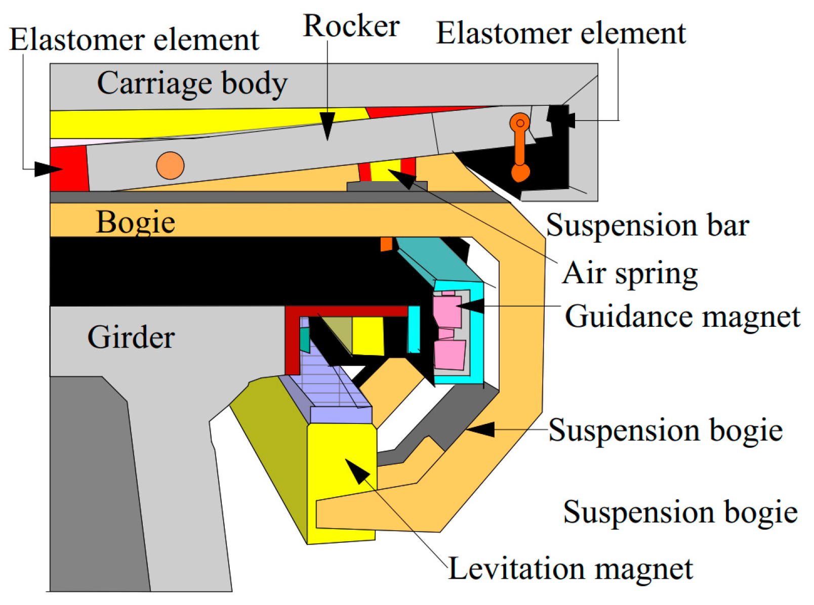
The high-speed magnetic levitation (maglev) train system employed in the SML consists of a total of five carriages, as seen in Figure 1a. The carriage body is equipped with four bogies, eight sets of rockers, fourteen complete sets, and four partial sets of electromagnets (levitation and guidance), as seen in Figure 1b,c and Figure A1. Each bogie consists of two C-shaped frames, as seen in Figure 2b. The two C-shaped frames are interconnected by a longitudinal shaft, resulting in the ability for the frames to rotate relative to each other while maintaining a fixed position in terms of translation. Levitation magnets and guiding magnets are affixed to the four bogies using rolling springs located on either side of the carriage. These magnets are evenly distributed over the full length of the vehicle, as seen in Figure 1c. The levitation magnets and guidance magnets establish a mutual interaction with the rails, which are modular functional components of the guideway inside the viaduct subsystem. This interaction occurs across a 10 mm air gap when the vehicle is in operation. The maglev train parameters used in this study are summarized in Table 1.
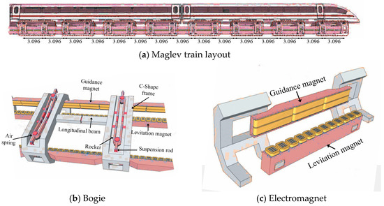
Figure 1.
Maglev train schematic diagram.
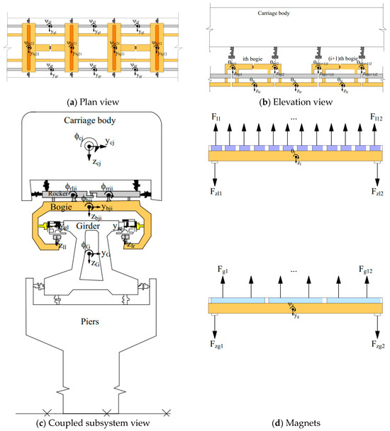
Figure 2.
Schematic modeling.

Table 1.
Maglev train parameters.
2.2. Establishment of the Maglev Train Model
The arrangement of twelve electromagnetic poles with equidistant spacing put on each levitation magnet is illustrated in Figure 1c. The pole pitch between these poles measures 0.258 m. The aforementioned poles serve as the primary components of electromagnetization that generate forces enabling levitation. Nevertheless, prior research on the interaction between the maglev train and the guideway has commonly employed a concentrated force model to depict the electromagnetic forces produced by the magnetic field between each magnet and rail [31,32]. The model incorporates electromagnetic poles, as seen in Figure 2a–d. In light of the intricate nature of the system and the inherent challenges in accurately representing every intricate aspect of the many components and linkages of the maglev train, the numerical model relies on the following assumptions. Therefore, this study assumes the utilization of linear elements for connecting the various components of the vehicles. These components are regarded as rigid bodies with limited and insignificant displacements and rotations.
The degrees of freedom (DOFs) associated with each part of the magnetic levitation (maglev) train system, along with their respective definitions of positive directions, are illustrated in Figure 2. The current investigation involves the modeling of the ith automobile body using five degrees of freedom (DOFs), namely vertical, lateral, roll, yaw, and pitch. These DOFs are represented by Equation (1). Each bogie consists of two C-shaped frames that are interconnected by a longitudinal shaft, enabling them to spin relative to each other without any translational movement. Hence, it can be observed that the ith bogie, situated beneath the jth train carriage body, possesses a total of six degrees of freedom. These degrees of freedom include roll, lateral, vertical C-shaped front frame, roll C-shaped rear frame, pitch, and yaw. This relationship is denoted by Equation (2). The C-shaped frame in Figure 2a accommodates two rocker arms, namely a left rocker arm and a right rocker arm, which are securely fastened in place. The degree of freedom (DOF) that is autonomous for each rocker arm is specifically associated with its rolling motion, whilst the remaining DOFs are interconnected with the DOFs of the bogie. Equation (3) represents the symbolic representations of the bearing rotations for the left rocker and the right rocker. Each combination of magnets, whether for levitation or navigation, is comprised of both a right magnet and a left magnet. Therefore, each levitation magnet is allotted two degrees of freedom (vertical displacement and pitch displacement), which are represented by Equation (4). In a similar manner, two degrees of freedom (DOFs) and yaw displacement are allocated to each guiding magnet as indicated by Equation (5).
The subscripts c, b, r, g, and l denote the train carriage body, carriage bogie, rocker, guidance magnet, and levitation (suspension) magnet, respectively. The subscripts “l” and “r” denote the left and right sides, respectively. The variable “i” represents the bogie number of the “j-th” carriage body, where “j” can take values of 1, 2, 3, or 4.
2.3. Equations of Motion for Maglev Train Vehicles
The determination of the equations of motion for each component of the maglev train is challenging because of the complexities associated with the train’s design. Therefore, the utilization of D’Alembert’s principle was initially employed to derive the equations of motion for individual rigid bodies comprising the train carriage. These equations were subsequently combined using MATHEMATICS software to formulate the equations of motion for the complete train carriage. The aforementioned concept can be articulated in the following manner:
In the given context, the symbol “” denotes the mass matrix of the maglev train carriage subsystem. Similarly, the symbols “” and “” represent the stiffness and damping matrix of the maglev train carriage subsystem, respectively. The symbols “”, “” and “” are used to represent the acceleration, velocity, and displacement vectors of the carriage subsystem. The symbol “” is employed to denote the interaction force vector between the maglev train carriage and guideway, while the symbol “” represents the external forces.
The motion displacement of the train system may be determined by considering the displacement vectors of each individual carriage, where “n” is the total number of carriages in the maglev train.
The term represents the displacement vectors of various components, including the carriage bodies, bogies, rockers, guiding magnets, and levitation magnets, that are present in the train consisting of “n” carriages. Furthermore, Equation (7) may be decomposed into “n” sets of terms representing the maglev train carriage bodies, bogies, and rockers, as well as “m” sets of terms representing the guidance and levitation magnets. It is important to note that .
where “k” denotes the number of magnets that are set.
The matrices and , representing the rockers and bogies of the jth maglev train carriage, can be enlarged in the following manner:
The displacement vectors, as described in Equations (7)–(11), are determined based on the degrees of freedom (DOFs) of the train components, as specified in Equations (1)–(5).
The mass matrix, as stated in Equation (6), may be assembled by combining the mass matrices of individual components of the train.
The term matrix represents the masses of the vehicle bodies, bogies, rockers, guiding magnets, and levitation magnets in a train consisting of “n” carriages. In accordance with Equations (8) and (9), the components of can be expressed in a more detailed manner as presented below:
The mass matrices, denoted as and , represent the rockers and bogies located in the jth maglev train carriage, respectively:
In a more specific manner, the mass matrices described in Equations (12)–(16) are also parameterized as follows:
The damping and stiffness matrices of the train, consisting of n maglev train carriage, have a comparable structure. The damping matrix, as stated in Equation (6), can be represented as follows:
where the sub-matrices are defined as follows:
The stiffness matrix KV can be obtained by simply replacing ‘C’ with ‘K’ in Equations (21)–(25).
3. The Maglev Viaduct System Modeling
3.1. The Maglev Viaduct System Constitution
The Shanghai Maglev Line (SML) is used as a reference to implement the 3D-finite element model of the maglev viaduct system. The overview of the maglev viaduct system, including its various components, is shown in Figure 3a. The rail, with a standard span of 3096 m and ensuring the functions of guiding and levitating the train, consists of eight modular functional units [33] (see Figure 3b). The rails, installed uniformly on each side of a girder concrete bearing and transferring the loads induced by the train to the piles, are maintained by four pairs of cantilevers per span. Such a combination of rails and girder concrete in box-shaped sections, also called hybrid guideway girders (HGG), is designed specifically for the maglev system [34]. HGGs are, in fact, a combination of prestressed concrete and rail that has been subjected to a modular construction application in which the connection between the concrete girders and the function unit girders (rail) is set up using brackets.

Figure 3.
Viaduct system.
The concrete girder is prestressed with centric pre-tensioning and then post-tensioned with tendons to help shape the girder. Thus, the applied pre-tensioning and post-tensioning methods reduce the impact of concrete shrinkage and creep on long-term track girder deformation and the transformation of concrete track girders into approximate elastic bodies. The prestressing arrangement adopts a pedestal pre-tensioning single bundle Φj15.24 steel hinge wire (some steel hinge wires are locally unbonded), multi-bundles of Φj15.24 steel hinge wires are pre-embedded and post-tensioned through corrugated pipes in the girder. The external bundle composed of multiple Φj15.24 steel strands is used as a backup measure in four forms of post-tensioning during the operation phase. The arrangement of pre-tensioned and post-tensioned prestressed steel bars for the track is shown in Figure 3c.
3.2. The 3D-Finite Element Model of the Maglev Viaduct System
On the SML, there are two types of sections: a bidirectional viaduct line supported by double column piers and a unidirectional viaduct line supported by single column piers. It’s easy to note that each girder is supported by its own column. Regarding the type of analysis to be performed in this study, the viaduct system with a single column pier was selected. Therefore, a 3D-finite element has been implemented to define the dynamic behavior of the viaduct referring to the SML. The flexibilities of the rails and the elements of modular functional units and supports are fully taken into account in the viaduct system numerical model (see Figure 4). The SML is composed of prestressed composite girders to reduce the effect of concrete shrinkage creep on the long-term deformation of the track girder and to transform the track girder concrete into an approximate elastic body. The girder is supported by square piles with a square base section 1.8 × 1.8 m in size and 10 m high. In this study, based on previous work, the influence of the pile foundation on the pile and on the soil was ignored, and the bottom of the pile was assumed to be fixed [35,36]. The steel laminated elastomeric bearings are designed with a plan dimension of 500 × 500 mm2 and a thickness of 40 mm to connect the girder to the pier. The flexibilities of both are therefore taken into account in the finite element model of the viaduct.
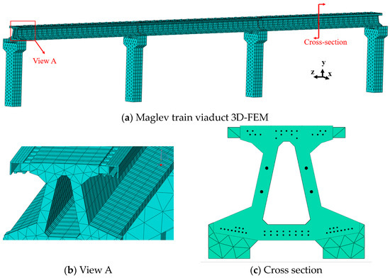
Figure 4.
Viaduct system modeling.
The rails of the HGG (Hybrid Guideway Girder) were specifically implemented in Abaqus using the Euler Bernoulli beam element model, based on the assumption that the plane cross-section perpendicular to the rail axis remains rigid, plane and perpendicular to the axis after deformation. The viaduct’s components, including the girder and pier, are modeled using an 8-node linear brick with reduced integration and hourglass control (C3D8R) in the mesh, with each node in the element having six degrees of freedom. The tie constraint is used to represent connections between rails and girders, with concrete girder elements acting as master and rail elements acting as a slave for connections. Because of its characteristic of deforming only by axial stretching, truss elements are suitable to model the reinforcement rod in order to simulate the dynamic behavior of the reinforced concrete girder. T3D2 truss elements were also employed for reinforcement. The friction surfaces between the concrete and the reinforcement were defined. Between the concrete and the reinforcement, a coefficient of friction of 0.6 was employed [37].
The consistency of the mesh size has some influence on the analysis result when analyzing a FE model. For the most precise results, meshing should be completed. Many researchers have investigated the best mesh size for a dynamic model. It was suggested in [38] to employ a mesh length of 20 mm in the flow direction and between 15 and 18 mm in the lateral direction in the loading region. The meshing size adopted in this FE model has been applied to improve the accuracy of the model results. Because the pressures and displacements were so great, a comparatively thin mesh was used along the route of the magnets. Near the loading area, a dense mesh was employed, whereas outside the loading region, a relatively coarse mesh was used.
3.3. Material Characterization and Viaduct Damping in Dynamic Analysis
The rail and reinforcements are assumed to be linear elastic in this study. The girder and pier concrete, which were assumed to be elasto–plastic, were modeled with concrete plastic damage in account. The reinforcement adopts Φj15.24 specification 270 level low relaxation seven wire smooth steel hinge wire. The tensile stress design for the first tensioning single bundle is 0.65~0.71 fpk (adjusted with temperature changes), the tensile stress for the first post-tensioning is 0.65 fpk, and the tensile stress for the second post-tensioning is 0.55 fpk. The maximum pre-applied stress of pre-tensioning and post-tensioning methods is less than 0.75 fpk [39]. Additionally, four linear spring-damper elements parameterized by the equivalent stiffness of the bearing are used to represent the bearing connected to the single-column pier in the vertical and lateral directions. More specifically, the stiffness of each spring-damper element in the vertical and lateral directions is respectively assigned to 4 × 10¹⁰ and 1.25 × 10¹⁰ N/m. The damping coefficient of each spring-damper element in the vertical and lateral directions is 1.2 × 10⁵ and 6 × 10⁴ N sec/m, respectively [36].
The damping of viaduct materials is one of the aspects that has a significant impact on the structure’s dynamic behavior. As a result, realistic structural damping in the dynamic analysis is required for an accurate modeling of the viaduct. The source of energy dissipation in the viaduct material can be modeled using damping rates. The Rayleigh damping matrix, represented in Equation (26), was utilized in this work to define the damping rate of the system with many degrees of freedom in Equation (28)
The symbol α is used to denote the mass damping coefficient, whereas β is used to indicate the stiffness damping coefficient. The determination of the damping coefficient that is proportionate to mass and stiffness may be achieved by the analysis of vibration modes and their corresponding particular modal damping ratio, as outlined below:
The vibration frequencies at the ith and jth modes are denoted as ωi and ωj, respectively. Similarly, the particular damping ratios at the ith and jth modes are represented by ξi and ξj, respectively. Within a specific range of frequencies, it is possible to estimate the damping rate as a constant value, whereas the damping coefficients exhibit identical critical damping ratios. Therefore, the expressions for mass and stiffness proportional damping may be reduced as follows:
The variables ω1 and ω2 denote the natural frequencies determined by modal analysis, whereas ζ denotes the crucial damping ratio for a certain order i.
The determination of the Rayleigh damping parameters is initially established by conducting a modal analysis using the numerical model developed in Abaqus. To ascertain the natural angular frequency ω (where ω = 2πf), the eight inherent frequencies were extracted. Hence, the value of the natural angular frequency ω1 was ascertained by the establishment of the fundamental natural frequency f1. Following the establishment of the fundamental frequency, the second angular frequency ω2 was ascertained by considering the highest natural frequency chosen among the vibration modes of different orders. It can be deduced that the natural angular frequencies ω1 and ω2, which are utilized in the computation of the Rayleigh damping parameters, are 18.012 and 40.071 rad/s, correspondingly. For the purposes of this investigation, the damping rate ξ of the structure was selected within the range of 1% to 3% on the basis of Peng-Fei et al.’s survey of data collection on a hundred highway bridges in China [40]. The Rayleigh damping coefficients α and β of the structure were determined by the utilization of Equation (28). The value of the damping coefficient proportional to mass α is determined to be 0.37279, whereas the damping coefficient β, which is proportional to stiffness, is calculated to be 0.00052.
4. Modelling Interaction of Maglev Train and Viaduct Contact Area
4.1. Interactive Model of Air Gap-Electromagnet Force
Magnetic levitation vehicles have no wheels, axles, or transmissions and rely on non-contact levitation, guiding, and propulsion technologies. Unlike traditional rail vehicles, the magnetic levitation vehicle has no direct physical contact with the guideway. Instead, these vehicles travel along magnetic fields produced between the vehicle and its rail, which are based on electromagnetic forces between the superconducting magnets on board the vehicle and the ground coils. Levitation coils are put on the guideway’s side walls. An electric current is created in the coils as the on-board superconducting magnets pass at high speed a few centimeters below the center of these coils, which then temporarily act as electromagnets. As a result, forces both push and pull the superconducting magnets upward. The opposing levitation coils are connected under the guideway rail, forming a loop. When a moving maglev vehicle, i.e., a superconducting magnet, moves sideways, an electric current is induced in the loop, resulting in a repulsive force acting on the levitation coils on the near side of the car and an attractive force acting on the levitation coils on the far side of the car. In this way, a moving car is always located in the center of the guideway. A repulsive force and an attractive force induced between the magnets are used to propel the vehicle (superconducting magnet). Propulsion coils located on the side walls on both sides of the rail are powered by three-phase alternating current from a substation, creating a changing magnetic field on the rail. The on-board superconducting magnets are attracted and pushed by the changing field, propelling the maglev vehicle.
Levitation and guidance magnetic forces are employed to establish contact between the maglev train and the viaduct rails. To simulate the levitation and guidance forces, this work adopts an interactive model between the electromagnet force and the air gap. Based on the current circuit and the air gap between the electromagnet and the rails, the electromagnetic force-air gap model is developed [41]
where (t) denotes the current time step and (w) denotes the wth maglev pole; denotes the current-controlled electromagnetic force between the wth maglev pole and the rail track; denotes the electrical intensity; denotes the magnetic air gap; K0 denotes the coupling factor related to the cross-sectional area of the core, calculated by ; Nm is the number of turns in the magnet winding; Aw is the area of the pole face; and μ0 is the air permeability. In Equation (29), the magnetic air gap is assessed by
where h0 represents the design static gap at the static equilibrium state of the maglev train which is 10 mm for SML; uw(t) represents the motion of the wth magnetic pole; represents the track deflection at the wth magnetic pole; represents the location of the wth maglev pole in the global X-coordinate; and represents the track irregularity.
In Equation (30), () and () are assessed directly from the dynamic analysis of the coupled system maglev vehicle and viaduct. In the static equilibrium, the maglev vehicle is levitated by the electromagnetic levitation force to balance the weight of the maglev vehicle. Such a levitation force is calculated by
where p0 (set to zero when Equations (29)–(31) are used) represents the weight of the train distributed at the wth maglev pole, and i0 represents the required value of the current to balance the maglev train weight and keep the design static gap h0.
To guarantee the safety and proper functioning of the railway system, a first control algorithm has been proposed to directly regulate the electromagnetic forces in order to ensure a constant force acting on the carriages and the tracks [42], followed by a second algorithm that adjusts the electromagnetic forces based on the carriage’s operating performance [43]. Furthermore, a PD controller is being developed to ensure that the air gap (roughly equal to h0) between the maglev pole and the track remains constant during maglev train operation.
This PD controller calculates the deviation error (expressed in Equation (31)) and then minimizes it by adjusting the current circuit.
The relationship between drive voltage and drive current at time should be considered before using the PD controller because of the importance of these values in controlling the maglev train system [44].
where represents the initial inductance of the coil winding of the guidance or levitation magnets; R0 represents the coil resistance of the electronic circuit; represents the static voltage; represents the control voltage of the wth maglev pole, which is determined by minimizing the gap error.
where Kd and Kp represent the derivative gain and the proportional gain, respectively. By replacing Equation (34) into Equation (33) and including , the control current is expressed as follows:
Since and are obtained from Equation (30) in the numerical study and represents the known current value at time t, the unknown control current at time can be determined by Equation (35). Finally, the levitation or guidance force at time can be determined from Equation (29).
Moreover, the track irregularities during operation were modeled using a 7-parameter power spectral density (PSD) function of the line irregularities.
where S(Ω) represents the line irregularities PSD (mm2 × m); Ω represents the spatial frequency (rad/m); and A, B, C, D, E, F, G represent seven characteristic parameters from Yau JD et al. work [45]. The wavelength defining the range of the PSD function is (0.258–150), thus implying a spatial step of 0.1. Thus, the profile of the runway irregularities was calculated and then shown in Figure 5, referring to the method of Ju et al. [46]. The maximum vertical and lateral irregularities are 1.211 and 3.273 mm, respectively.

Figure 5.
Time sequence sample of track irregularities.
4.2. Motion Equations of Coupled Maglev Train-Viaduct System
The equations of motion of the maglev train-viaduct system are described as follows:
where represents the electromagnetic forces vector acting on the maglev train carriage, the value of which is determined by Equation (7), with non-zero inputs corresponding only to levitation and guidance magnets and inputs for carriage bodies and other elements corresponding to zero. For , it represents the electromagnetic forces vector acting on the viaduct, with non-zero parts directed towards the loading rails and determined by the moving loads’ position vectors acting on the rails due to the magnetic levitation train system, whose inputs are equal to zero for the other elements of the viaduct.
Assuming n, the number of carriages in the maglev train operating on the viaduct, the total number of maglev poles arranged on the m sets of magnets is defined by with the interactive electromagnetic force generated between the zth pole of the magnetic levitation transport system and the rail represented by a concentrated force . All electromagnetic forces are first calculated on the basis of the control algorithm and the feedback from the coupled subsystem at time t for a time increment . Thus, these electromagnetic forces representing the resultant external forces of each magnet are then grouped into the vector at the relevant DOFs of each magnet in order to calculate the responses of the maglev train carriages at time . Meanwhile, the electromagnet forces, constituting the non-zero inputs to the vector, are determined by the position vectors of the moving loads acting on the rails defined as follows.
where v represents the operating speed of the maglev train; represents the travel time of the zth pole on the relevant span of the viaduct, represents the force space; L represents the length of a span of the girder; H(t) represents the unit pitch function; and n is the number of spans. The interactive electromagnetic forces at time , obtained using Equations (29)–(33) in which the PD controller is used to adjust the interaction forces as a function of the deviation error , have been established through the development of a Dload interface to simulate train operation by the position vector with . Thus, the subroutine to specify the distributed forces in the electromagnetic field between the vehicle and the guideway (DLOAD), which allows users to specify the variation in the distributed electromagnetic forces as a function of time and magnet position, are based on the set of equations mentioned above.
5. Validation of the Numerical Model
5.1. Comparative Analysis between Field Measurements and the 3D-FEM Result
The 3D-FE model was validated in two stages, which are described below.
- Stage 1
The Shanghai Maglev Line (SML) was subjected to field vibration measurements in the first phase. Vibration measuring devices were installed throughout the system during the SML vibration measurement experiment. One of these measurement locations set mid-span under the girder and equidistant from the two rails (as shown in Figure 6), was chosen to conduct the comparative study of field data and the proposed numerical model results. INV9828 series accelerometers with a frequency response range of 0.2 to 2500 Hz, a measurable acceleration field of 0.1 to 10 g, a sensitivity of 500 mV/g, a working current range of 2 to 20 mA, an operating voltage range of 18 to 28 VDC, an output impedance of 100, an operating temperature range of 40 to 120 °C, and an impact limit of 1000 g were used. The sensor frequency was set to 500 Hz for the field measurement while the maglev train was traveling at roughly 340 km/h.
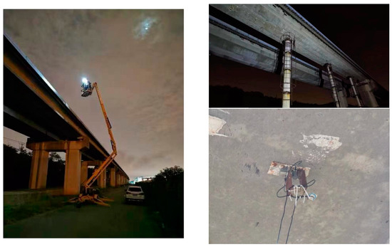
Figure 6.
Field test device layout.
Figure 7 depicts the dynamic acceleration at mid-span below the girder. Under the action of electromagnetic forces caused by maglev train operation, the periodic generation of wave series can be noticed. When the train magnets are in the area above the measuring location, acceleration maxima are recorded in defined time histories corresponding to the maglev train passage over the viaduct. Furthermore, there was a strong correlation between the data collected in the field and the results obtained using the FE model. In order to assess the error rate between the data recorded in the field and the values calculated using the numerical model, the RMS of the vibration in the time domain of each data was first evaluated, then the discrepancy between the field data and those of the numerical model was determined by calculating a difference rate d (). Thus, the measured dynamic acceleration RMS is 0.3808 m/s2, and the assessed dynamic acceleration RMS is 0.3616 m/s2. On average, the indicated difference is 7.26%.
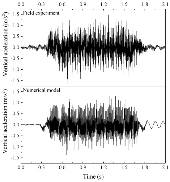
Figure 7.
Vibration acceleration time history at midspan under girder.
Figure 8 depicts the frequency spectrum at mid-span below the girder. The data measured in the field and the findings assessed using the numerical model were found to be very similar. The measured acceleration amplitude RMS is 0.0158 m/s2/Hz, whereas the computed acceleration amplitude RMS is 0.0147 m/s2/Hz. On average, the indicated difference is 6.96%.
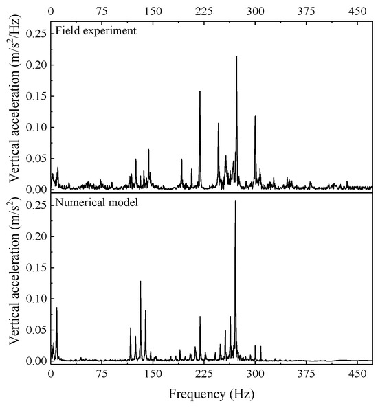
Figure 8.
Vibration acceleration spectrum at midspan under girder.
- Stage 2
This second level of numerical model validation is based on Z. L. Wang et al.’s [44] and Shi’s numerical model [31]. At this point, only the vertical displacement time history was investigated because it was the only data available from earlier research to validate the numerical model’s results in the context of this work. A five-car maglev train is also utilized on this SML, which travels at 430 km/h through the test site. A measurement point was placed at the top girder midspan to record the vertical displacement of the viaduct system under the moving load of the maglev train.
Figure 9 depicts the dynamic displacement at the top girder’s midspan. In terms of the evolution of displacements over time, the three curves are identical in time, form, and magnitude with respect to the period before loading, full loading, and after loading of the girder. The numerical model created vibrates around a slightly lower value of 1.55 mm, whereas Shi’s model and Wang’s field measurements are 1.42 mm and 1.53 mm, respectively, representing a difference of 8.38% and 1.29%.
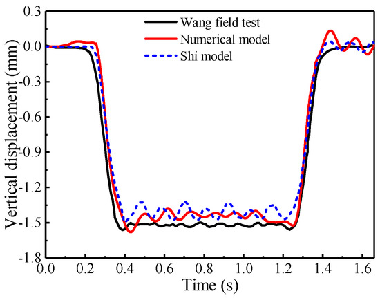
Figure 9.
Vertical displacement at the girder midspan.
When the data from Stages 1 and 2 are combined, the causes of the observed variations could be attributable to some of the criteria listed below:
- (1)
- The targeted speed fluctuated since it was impossible to keep the maglev train’s speed consistent during operation.
- (2)
- When the maglev train approaches, the sensors are subjected to vibrations, which continue even after the magnet passes. As a result, the sensors’ reaction is compromised. The disparity between the inclination of the spikes in the 3D-FE model result and the vibrations in the field measurement is seen here.
- (3)
- Rayleigh damping parameters are based on a modal study of the entire system, although in practice, each material responds differently depending on its damping.
- (4)
- The possible external traffic impact on the collected data, whereas the ground effect, is not taken into account in this investigation.
5.2. Correlation Analysis between the 3D-FEM Results and Field Data Test
The comparison of field test data and numerical results demonstrates that the 3D-FE model developed in Abaqus accurately predicts the dynamic response of the maglev viaduct system. Nonetheless, there remains a little margin of error in terms of curve shape and amplitude. A correlation study with all variables was done to assess the impact of these observed discrepancies on the model’s accuracy in predicting the dynamic response of the structure. The recorded vibration accelerations from the numerical model calculation and field tests were processed. The coefficient ϒUV is used to calculate the correlation between two variables, u and v.
where
denotes the mean of u; and
denotes the mean of v
The Pearson coefficient of correlation yields a value in the range (−1;1); the sign reflects the direction of the association. However, r = 0 indicates that there is no linear relationship. Table 2 shows the degree of correlation between the FE model’s results and the measured field data.
Table 2.
Correlation matrix of measured data and computed results.
The correlation factor varies between 0.988 and 0.907 depending on the location, according to the presentation of the correlation matrix of the vibration accelerations obtained during the field testing and the results of the FE model. Thus, at the level of 0.001, the dynamic response of the viaduct system computed by the FE model and the vibrations noted during the field test at different sites had a very significant correlation. As a result, the disparity in the form and size of the curve between the FE model results and the field data has no effect on the FE model’s capacity to effectively predict the dynamic response of the maglev viaduct system during maglev train operation.
6. Pultruded FRP Rod Performance Analysis in a Maglev Viaduct in Operation
6.1. Pultruded FRP Characterization and Modelling
This study evaluated two types of fiber materials (polyacrylic nitrile carbon, High Modulus, and S-Glass, as indicated in Table 3) to evaluate the performance of pultruded FRP bars. In general, the material properties of pultruded FRP bars can be determined using a burning test and an analytical micromechanical model. Pultruded FRP bars are made of longitudinal fiber for tensile strength, transverse felt for stiffness and impact resistance, and injected matrix material for corrosion resistance, particularly against external impacts. The longitudinal fibers are the primary determinant of the mechanical behavior of FRP-pultruded bars. As a result, knowing the fiber ratio in the rod is required to investigate its influence on the material’s behavior. Thus, the component ratio of pultruded FRP used in this study was based on the results of the burn-off test performed by Carlos et al., who found a fiber and matrix volume fraction of 82.45% and 17.55%, respectively, with the fillers accounting for 17.5% by weight of the pure resin of calcium carbonate fillers [47]. To achieve effective material properties, the mixture rule, which is one of the common methodologies used to evaluate the properties of unidirectional fiber-reinforced composites and is also known as Voigt’s formula and was proposed by Voigt and Reuss, was utilized. The modulus of elasticity of fiber-reinforced composites can be computed as follows:
where “(…)f” and “(…)m” denote the fiber’s and matrix’s elastic properties, respectively. These properties are represented by “E(…)(…)”, “V(…)”, “v(…)(…)” and “G(…)(…)”, which stand for Young’s modulus of fiber, the volume fraction of fibers, Poisson’s ratio of fiber, and shear modulus of fiber, respectively. Fiber-reinforced composite materials are often composed of stiff, strong fillers with tiny diameters inserted in a variety of matrix phases. Table 3 shows the mechanical parameters of pultruded FRP employed in the numerical calculation. It should be mentioned that for each type of model run, a modal analysis was performed to identify the damping parameters.
Table 3.
FRP material mechanical properties.
6.2. Dynamic Response of the Maglev Viaduct System
Few studies have been conducted on the effect of traffic speed on the stress-strain response of a railway viaduct. Eleven distinct traffic speed levels (5 to 500 km/h) were evaluated in this study to examine the effect of maglev train speed on the dynamic response of the structure. Figure 10 depicts the spectrum of the maximum dynamic strain at the upper surface of the second girder during a maglev train operating at 400 km/h. As can be seen, the dynamic strain normally grows higher from the bare piers to the girder’s mid-span, with the highest maximum strain noticed at the longitudinal edges at the girder’s mid-span. This is affected by the position of the rails, whose supports are attached to the girder’s sides. The load borne by the rails is thus dispersed to the ground by the girder-piers transmission system during maglev train operation. As a result, the maximum dynamic strain at mid-span in the middle of the girder is not as great as it is at mid-span at the edge. This highlighted the importance of taking the hybrid-guideway girder into account in the development of the Shanghai maglev viaduct 3D-FE model for more realistic results. Nonetheless, due to its location a little distant from the girder flank, the mid-span center of the girder will be investigated in the current analysis, reflecting roughly the average of the entire construction in terms of values.
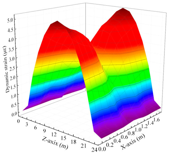
Figure 10.
Peak strain amplitude at the girder top.
Figure 11 depicts a typical time history of vertical displacement and dynamic pressure at the specified spot when the maglev train is traveling at 400 km/h. The dynamic pressure and vertical displacement time histories can be seen to evolve in three phases (pre-load, full load, and post-load), with peaks regularly observed at the passage of a carriage in the vicinity of the selected point, which almost cancels out when the carriage in the train moves away. The dynamic pressure time history at the girder’s mid-span is dominated by a compressive component that stabilizes at the end of the load to become tensile components after the passing of the maglev train, i.e., after the full loading period. In contrast, the vertical displacement time history at the girder’s mid-span is dominated by a tensile component that stabilizes at the end of the load to become compressive components during the maglev train’s passage, i.e., after the full loading period.

Figure 11.
Strain-stress time history of the conventional system at a speed of 400 km/h.
The maximum peak of the dynamic response of the structure was analyzed using the fast Fourier transform approach due to the shape of the pressure and displacement curves, which have tensile and compressive components. Figure 12 depicts the peak dynamic pressure amplitude and peak vertical displacement amplitude response as a function of maglev train speed at the girder’s mid-span. It is noted that the highest value of the vertical displacement and dynamic pressure at the girder’s mid-span increases as the speed of the load-controlled maglev train increases. At the given maglev train speeds, the displacement amplitude peak and the pressure amplitude peak follow the same pace, including the dynamic amplification phenomenon. The dynamic pressure amplitude peak grows from 12.6312 × 10⁴ Pa/Hz to 12.9997 × 10⁴ Pa/Hz when the train speed increases from 5 km/h to 500 km/h, as seen on the graph. Similarly, the maximum vertical displacement amplitude rises from 0.740187 × 10⁻³ m/Hz to around 0.740647 × 10⁻³ m/Hz. This type of analysis, which results in the same displacement and stress rate, has also been addressed by Jing Hu et al. [48] in their work on the dynamic response of a ballasted railway to a moving train and by Jiaqi Guo et al. [49] in their work on the dynamic response of a tunnel subjected to a moving train. The dynamic amplification phenomenon that occurs as train speed increases is caused by the system’s natural frequencies combined with the load distribution of the five carriages on the rails, which coincide with the frequency of the train’s moving load, as defined by Zenong Cheng et al., who show that the bridge amplification factor is a function of the length ratio between the bridge span and the vehicle [50]. Thus, the results of the analyses are fully justified because the frequency of the moving magnetic levitation train’s load increases as the operating speed increases; this directly leads to an approach to the natural frequency of the structure, where the vibrations increase, and then to an eventual move away from the natural frequency of the structure, where the vibrations decrease after reaching a certain peak.
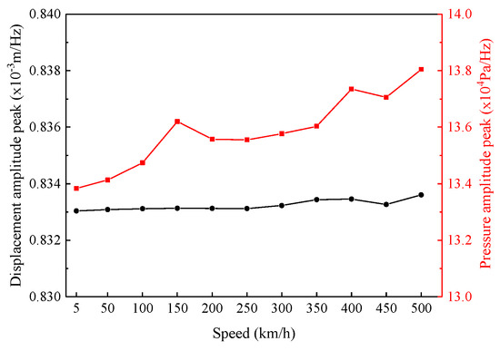
Figure 12.
Strain-stress peak of the conventional system.
The dynamic response of the viaduct when reinforced with steel bars and when reinforced with FRP bars is analyzed in the second half of this section. To evaluate the FRP performance in the viaduct during maglev train operation at different speeds, two types of FRP were used. This section explored the girder vertical displacement during maglev operation. Figure 13 shows that the vertical displacement amplitude at the girder’s mid-span follows nearly the same pace for all forms of reinforcement utilized, although the displacement level differs depending on the type of reinforcement used. When reinforced with PNCFRP, the structure displacement is reduced under train dynamic load. When the steel is replaced by S-GFRP, the peak vertical displacement amplitude increases significantly. At a speed of 300 kmh, the maximum displacement amplitude of a PNCFRP-reinforced girder is approximately 87.87% of that of a steel-reinforced girder. The maximum displacement amplitude when the girder is reinforced with S-GFRP, on the other hand, is 109.34% of that when reinforced with steel. Based on this research and the mechanical properties of the materials utilized, the stiffness of the materials governs the displacement of the structure. As a result, the structure reinforced with the most rigid material experiences the least displacement. In this way, the use of high-stiffness fibers improves the structure’s rigidity and, as a result, significantly contributes to the structure’s ability to endure displacement generated by a dynamic train load.
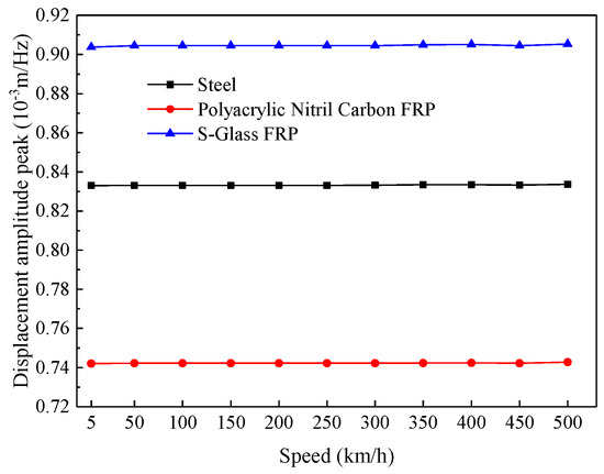
Figure 13.
Amplitude displacement peak at the girder midspan.
Figure 14 depicts the spectrum of the acceleration amplitude at the mid-span of the girder during the passage of the maglev train at various speeds. As can be seen, the structure’s vibration frequency increases with operation speed. Furthermore, when the train speed increases, there is an increase in periodic amplitude cycles, as evidenced by a sharpening of the amplitude peaks at each periodic amplitude cycle. The acceleration amplitude spectrum at the girder’s mid-span changes depending on the material applied to reinforce the structure. Thus, the graph in Figure 14d has been generated based on the value of the maximum peak in acceleration amplitude.
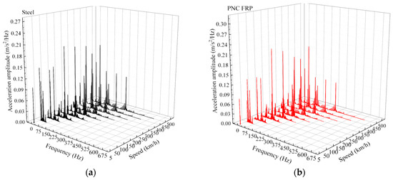
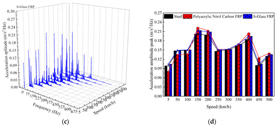
Figure 14.
Acceleration amplitude spectrum at the girder midspan at various maglev train speeds. (a) Acceleration amplitude spectrum for steel-reinforced girder concrete structure; (b) Acceleration amplitude spectrum for CFRP-reinforced girder concrete structure; (c) Acceleration amplitude spectrum for GFRP-reinforced girder concrete structure; (d) Peak amplitude according to speed.
Although the variation in maximum peak for each structure type is minor, it should be noted that the mechanical properties of the reinforcement materials influence the structure’s acceleration. Thus, the peak acceleration amplitude at the girder’s mid-span fluctuates with the maglev train’s operating speed, following the same pattern as displacement. The impact of the reinforcements on the acceleration amplitude spectrum of the girder is irregular, as illustrated in Figure 14d. At speeds of 5, 50, and 100 km/h, the S-Glass-reinforced structure has a high peak of acceleration amplitude, whereas the PNC FRP-reinforced structure has a low peak of acceleration amplitude, indicating that the structure is governed by stiffness (for example, at 5 km/h, the acceleration amplitude peak of the S-Glass-reinforced structure is 106% of that of the steel-reinforced structure whereas the acceleration amplitude peak of the PNC FRP-reinforced structure is 80.5% of that of the steel-reinforced structure). For speeds between 150 and 500 km/h, the steel-reinforced structure has a low peak, while the PNC FRP-reinforced structure has a high peak, indicating that the structure is governed by its weight (for example, at 500 km/h, the acceleration amplitude peak of the S-Glass-reinforced structure is 104% of that of the steel-reinforced structure, whereas the acceleration amplitude peak of the PNC FRP- reinforced structure is 108% of that of the steel-reinforced structure). In contrast to displacement amplitude, which is determined by structural stiffness at all operating speeds used in this study, acceleration amplitude is determined by both structural stiffness and mass. The influence of reinforcement in the structure is strongly reliant on the frequency of the moving load, according to this investigation. The variance in reinforcement impact during the maglev train operation at varied speeds due to the irregularity of the computed acceleration amplitude peaks, the variance in reinforcement impact during train operation at varied speeds might be attributed to the natural frequencies of each viaduct, depending on the type of reinforcement applied, might be attributed to the natural frequencies of each viaduct, depending on the type of reinforcement applied. This causes a value coincidence: as one curve declines toward its minimum after reaching its extreme, the other may be rising towards its peak. It is also worth noting that, according to Zenong Cheng, who researched the dynamic amplification of a beam under a moving load [50], a bridge structure can experience numerous resonances at different moving load speeds.
6.3. Extreme Response Analysis of the Girder Subject to a Maglev Train Carriage
The extreme response of the maglev girder is analyzed in this section to verify the hypothesis advanced above, which explains the irregularity of the peak acceleration amplitude depending on the type of reinforcement (steel, polyacrylic nitrile carbon FRP, and S-glass FRP) used when the maglev train operates at different speeds. For that purpose, the Moving Load Amplitude Spectrum (MLAS) method of resonance analysis of a supported bridge in the frequency domain is used. To reduce computation time and complexity, the girder’s cross-section is changed while preserving the trapezoidal appearance with a 12 m span. The simply supported girder is considered to be an Euler–Bernoulli beam with constant section bending stiffness (), unit mass (), and damping () throughout the span direction. The traveling load is comparable to that of a single-car maglev train. The load distribution under the carriage, on the other hand, is regarded as a concentrated load under each magnet. As illustrated in Figure 15, the moving load model is made up of a succession of moving concentrated forces Pi (i = 1, 2, 3,…, Jp) with equal spacing d, i.e., equidistant moving concentrated forces numbering Jp and total length Lc (). The equation of motion for a simply supported girder of span L subjected to equidistant concentrated forces moving at speed v is as follows:
where is the vertical displacement of the girder at a position and time ; is the moving carriage load at a position of the girder and time ; is the distance between the ith moving concentrated force and the first concentrated force ; is the time when the ith moving concentrated force reaches the end of the girder; is the Dirac function, , where represents the Heaviside function.
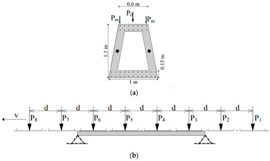
Figure 15.
Simply supported beam subject to the train dynamic load. (a) Typical cross-section of the beam; (b) Simple beam subject to a row of load.
The vertical displacement at girder position can be represented using the mode superposition approach as the multiplication of the generalized coordinate and the mode function , i.e.,
By replacing Equations (46)–(48) into Equation (45), in accordance with the orthogonality of the modes, it can be defined that:
where and are, respectively, the nth mode damping ratio and the circular frequency of the girder, is the nth-order mode load of the moving vehicle forces. The nth-order response component in the frequency domain can then be defined by the Fourier transform of Equation (49).
where represents the transfer function
And represents the spectrum of the moving load, which is related to the moving loads and the girder mode function obtainable by the Fourier transform of via the adoption of the moving load model. For a simply supported girder with mode function , when the equidistant moving concentrated forces , the moving load spectrum is presented as follows:
Furthermore, with the odd n mode is expressed as follows.
While with mode n even is expressed as follows.
Then, the girder displacement response spectrum under equidistant moving loads can be expressed as:
The corresponding girder acceleration response spectrum can be obtained by differentiating the displacement twice with respect to frequency:
In the case of simply supported bridges, accuracy requirements can be addressed by considering only the first-order bridge mode [51]. Higher-order modes and structural dampening are thus ignored in the resonance analysis of simply supported bridges subjected to equidistant moving loads in order to simplify computations. As a result, the following is the amplitude spectrum of the girder acceleration response generated by equidistant moving loads:
For the calculation of the structure’s natural frequency, the lumped mass matrix approach method was adopted. Some assumptions have been made to the simple supported reinforced concrete beam subjected to free vibration and listed as follows:
- The mass (m) of the entire system is considered to be lumped in the middle of the reinforced concrete beam.
- No energy-consuming elements are present in the system.
- The reinforced concrete is considered a composite material whose mechanical properties can be determined using Voigt’s method.
- The governing equation of such a system (mass-spring system without damping in free vibration) using a mass matrix approach is the following:
The characteristic equation is given by:
The stiffness matrix [K] and the mass matrix [M] are determined, respectively, as follows:
The stiffness matrix [K] of the entire beam is determined as follows:
For element 1, the boundary condition described in Figure 16 is applied and the elimination approach is used.
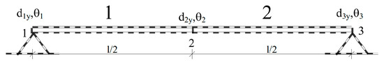
Figure 16.
Finite element discretization of the beam.
For element 2, the boundary condition described in Figure 16 is applied and the elimination approach is used.
Replacing Equations (49) and (51) in Equation (47),
The lumped mass matrix [M] of the reinforced concrete beam is determined as follows:
For element 1, the boundary condition described in Figure 16 is applied, and the elimination approach is used.
For element 2, the boundary condition described in Figure 16 is applied, and the elimination approach is used.
Replacing Equations (56) and (58) in Equation (54):
Replacing Equations (53) and (60) into Equation (46) gave:
Then,
Knowing that can also be expressed as
The analytical model of a simply supported bridge reinforced with steel was validated by comparing the maximum acceleration amplitude estimated by a numerical model developed in Abaqus with the maximum acceleration amplitude computed by the analytical model, as summarized in Table 4. The comparative study was carried out for moving concentrated force speeds of 50 km/h, 150 km/h and 250 km/h. The results show that an error rate varying between 7.37% and 8.41%, perhaps justified by the method of quantifying the mechanical properties of the composite, was observed. Thus, this analytical model can be used for further study.
Table 4.
Analytical model validation error recorded.
The peak of the acceleration amplitude spectrum (Figure 17) investigation reveals resonance phenomena at various speeds based on the type of reinforcement used in the structure during speed variation, as well as irregularities in the dominance of the acceleration amplitude peak values. The peak acceleration amplitude is governed by the stiffness of the structure at very low speeds, as observed, because in the 0–25 km/h range, the peak acceleration amplitude is minimal for the polyacrylic nitrile carbon high modulus-reinforced structure but high for the S-Glass-reinforced structure. This occurs due to the structure’s quasi-static characteristic, which vibrates slightly at low operating speeds. Beyond this speed range, the steel-reinforced structure encounters its first resonance occurrence, which happens early in the S-Glass-reinforced structure and late in the PNCFRP-reinforced structure. Depending on the type of reinforced girder concrete, this resonance phenomenon occurs in the same order throughout the curve. The natural frequency of the structure is accountable for the phenomenon of resonance occurring at different speeds depending on the type of structure, which is 57.535 s−1, 63.229 s−1, and 56.822 s−1 for steel-reinforced girder concrete structure, PNCFRP-reinforced girder concrete structure, and S-Glass FRP-reinforced girder concrete structure, respectively. Thus, the higher the natural frequency of the structure, the later the resonance phenomenon occurs, which explains the higher speed resonance occurrence in this case whenever the structure is reinforced with polyacrylic nitrile carbon.
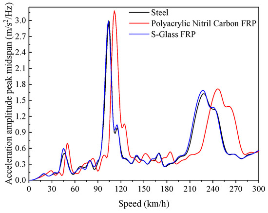
Figure 17.
Peak acceleration amplitude according to speed.
Nevertheless, it should be noted that the acceleration amplitude values in the resonance zone are strongly dependent on the weight of the structure. In other words, the lighter the structure, the greater the acceleration amplitude in the resonance zone. Consequently, the weight of the structure plays an important role in reducing the peak acceleration amplitude of the system in the resonance zone. Thus, the use of lightweight fibers to replace steel in a concrete structure needs to be channeled. The resonance zone of the structure must be avoided in order to prevent the resonance that occurs, which could be strong compared to that of a structure reinforced with steel. This means that dynamic movements on structures must be performed at frequencies not close to the structure’s resonance frequencies. In another case, if the FRPs are to be used due to environmental problems or to reduce the displacement of the system (in the case of high-rigidity fibers), it is advisable to increase the volume of concrete to even out the weight deficit in case the dynamic load frequency cannot be controlled.
7. Conclusions
Assessment of the dynamic behavior of the viaduct induced by the maglev train operation when steel-reinforced concrete is replaced by FRP-reinforced concrete was explored using an Abaqus non-linear 3D finite element model. By comparing simulation findings to field test data, the reliability of the numerical model, which was built in line with the size and conditions of the Shanghai maglev train viaduct section, was validated. The electromagnetic forces acting in the interaction zone between the magnet poles beneath the train and the rails were incorporated into the numerical model using a Fortran DLOAD subroutine. The vibrations of the girder during operation on the viaduct, whose concrete is reinforced with polyacrylic nitrile carbon FRP bars or S-glass FRP bars, were analyzed after the numerical model was successfully validated following calibration. As a result, the following conclusions can be drawn:
- The comparison of the calculated acceleration and displacement histories with those measured at the girder’s mid-span reveals a good correlation with a slight error rate, defining the model’s reliability to accurately simulate the dynamic behavior of the girder during maglev train operation on a viaduct. This leads to a first observation about the direct dissipation of the load carried by rails on the ground by the girder-piers transmission system because the maximum dynamic strain in the middle of the girder at mid-span is not as great as that at the girder’s edge (rail position) at mid-span, thus justifying the importance of taking the hybrid-guideway girder into account in the development of the Shanghai maglev viaduct 3D-FE model for more realistic results.
- The analysis of the girder’s dynamic response at midspan reveals a time-history evolution of dynamic pressure in three phases (pre-load, full-load, and post-load), dominated by the compressive component in the full-load period, then stabilizing at the end of the load to be dominated by the tensile component in the third period. A similar phenomenon of phase change over time is observed in the case of the vertical displacement of the girder at mid-span, the amplitude of which increases with maglev train speed, with the detection of dynamic amplification at certain speeds.
- The study of the influence of FRPs (polyacrylic nitrile carbon and S-glass) used to replace steel in reinforced concrete reveals that the stiffness of the materials utilized governs the vertical displacement of the structure. Indeed, at all study speeds, the structure reinforced with polyacrylic nitrile carbon FRP (high elasticity) has minimal displacement, but the structure reinforced with S-Glass (low elasticity) experiences significant displacement. The use of high-rigidity fibers thus contributes significantly to the viaduct’s ability to withstand the displacements generated by maglev train operation.
- An examination of the acceleration amplitude spectrum indicates an irregularity in the efficiency of FRPs in replacing steel to reinforce the viaduct girder’s concrete. The impact of FRPs varies depending on the speed studied; that is, there are train operating speeds for which the structure is governed by the stiffness of the materials, while for other train operating speeds, the structure is governed by the weight of the structure. As a result, the impact of reinforcing the concrete girder of the viaduct with FRPs is significantly dependent on the frequency of the moving load.
The extreme response of the viaduct is evaluated using an analytical method that considers the structure as a simply supported beam with modified dimensions and subjected to a moving maglev train carriage, which leads to the following findings:
- The use of high-stiffness FRPs is effective for bridges subjected to very low dynamic load frequencies due to the quasi-static behavior of the structure. Thus, the acceleration of the structure governed by the stiffness of the materials is minimal for high-stiffness FRPs.
- As operating speed increases beyond the quasi-static period of bridge behavior, resonance phenomena dependent on the natural frequency of the structure begin to occur. As such, a structure with a high natural frequency experiences dynamic amplification later on; this results in a lack of constancy in the effectiveness of high-rigidity FRPs in replacing steel, as (1) an FRP-reinforced bridge may experience resonance phenomena before or after the steel-reinforced bridge during train operation, (2) the period when the acceleration amplitude of the FRP-reinforced structure falls after reaching its peak may coincide with the period when the acceleration amplitude of the steel-reinforced structure rises. This means that particular attention must be paid to the frequency of dynamic loading to which the bridge is subjected in order to take advantage of the periods when FRP is effective.
- The amplitude of acceleration in the resonance zone is strongly dependent on the bridge weight. In other words, the lighter the bridge, the greater the acceleration amplitude in the resonance zone. Consequently, the use of lightweight fibers to replace steel in the bridge girder concrete must be channeled in such a way as to avoid resonance speeds during train operation or to increase the concrete volume to compensate for the weight deficit in the event that the frequency of the dynamic load cannot be controlled.
This study, which focuses on the components of a viaduct’s dynamic response, could be useful in bridge design. This research has revealed that viaduct displacement and acceleration vibration are regulated by various factors. To optimize a viaduct’s dynamic response, specifically its displacement and acceleration, several parameters must be considered, including structure stiffness, structure mass, structure natural frequency, and frequency of the dynamic load to which it is subjected. Thus, when subjected to dynamic loading, the adoption of bridges with concrete components reinforced with FRP rather than steel proves beneficial. This study adds to prior research on the application of FRP bridges by describing the various circumstances in which FRP structures are efficient.
8. Work Limitation
Some limitations were recorded while modeling the maglev train and are presented as follows:
- (1)
- The rigid body hypothesis is employed to model the primary components of the train system, implying that the elastic deformation of these components is ignored.
- (2)
- Linear spring elements are employed to model the train subsystem’s rigid body connections.
- (3)
- Throughout the dynamic analysis, rigid body displacements and rotations are considered to be low.
- (4)
- Due to the intricacy of the girder’s constitution, the analytical model of the Hybrid-Guideway Girder was simplified in a simple supported beam of trapezoidal shape.
Author Contributions
Conceptualization, I.V.L.C. and J.C.; methodology, I.V.L.C. and J.C.; software, I.V.L.C.; validation, I.V.L.C. and J.C.; formal analysis, I.V.L.C.; investigation, I.V.L.C. and J.C.; resources, J.C and Z.H.; data curation, I.V.L.C. and Z.H.; writing—original draft preparation, I.V.L.C.; writing—review and editing, I.V.L.C. and J.C.; visualization, I.V.L.C.; supervision, J.C.; project administration, J.C.; funding acquisition, J.C. and I.V.L.C. All authors have read and agreed to the published version of the manuscript.
Funding
This research was funded by the National Natural Science Foundation of China (Grant No. 52178151); Shanghai TCM Chronic Disease Prevention and Health Service Innovation Center (Grant No. ZYJKFW201811009); State Key Laboratory for Disaster Reduction of Civil Engineering (Grant No. SLDRCE19-B-22) and Shanghai Post-Doctoral Excellence Program (Grant No. 2022519).
Data Availability Statement
The data presented in this study are available on request from the corresponding author. The data are not publicly available due to privacy.
Conflicts of Interest
The authors declare no conflict of interest.
Nomenclature
| Mass matrix of the maglev train carriage subsystem | Stiffness matrix of the maglev train carriage subsystem | ||
| Damping matrix of the maglev train carriage subsystem | Acceleration vectors of the carriage subsystem | ||
| Velocity vectors of the carriage subsystem | Displacement vectors of the carriage subsystem | ||
| Interaction force vector between the maglev train carriage and guideway | External forces | ||
| Motion displacement matrice of the train system | Rockers displacement matrice of the jth maglev train carriage | ||
| Bogies displacement matrice of the jth maglev train carriage | Mass matrice of the train system | ||
| Rockers mass matrice of the jth maglev train carriage | Bogies mass matrice of the jth maglev train carriage | ||
| ξ | Damping ratio | ω | Natural angular frequency |
| α | β | ||
| t | Current time step | Current-controlled electromagnetic force between the wth maglev pole and the rail | |
| Electrical intensity | Magnetic air gap | ||
| K0 | Coupling factor related to the cross-sectional area of the core | Nm | Number of turns in the magnet winding |
| Aw | Area of the pole face | μ0 | Air permeability |
| uw | Displacement of the wth magnetic pole | uG | Track deflection at the wth magnetic pole |
| Location of the wth maglev pole in the global X-coordinate | Track irregularity | ||
| Initial inductance of the coil winding of the magnet | R0 | Coil resistance of the electronic circuit | |
| Static voltage | Control voltage of the wth maglev pole | ||
| Electromagnetic forces vector acting on the maglev train carriage | Electromagnetic forces vector acting on the viaduct | ||
| Vertical displacement of the girder at a position x and time t | Moving carriage load at a position x of the girder and time t | ||
| Distance between the ith moving concentrated force and the first concentrated force | Time when the ith moving concentrated force reaches the end of the girder | ||
| Dirac function | Heaviside function | ||
| Generalized coordinate | Mode function | ||
| nth mode damping ratio | Circular frequency | ||
| nth-order mode load of the moving vehicle forces | Transfer function | ||
| Spectrum of the moving load | Girder acceleration response spectrum |
Appendix A
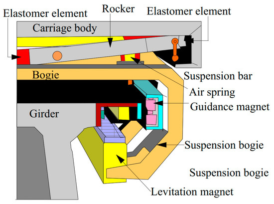
Figure A1.
Cross-section of the coupled maglev train viaduct subsystem.
Figure A1.
Cross-section of the coupled maglev train viaduct subsystem.
References
- Van Den Einde, L.; Zhao, L.; Seible, F. Use of FRP composites in civil structural applications. Constr. Build. Mater. 2003, 17, 389–403. [Google Scholar] [CrossRef]
- Karbhari, V.; Seible, F.; Burgueno, R.; Davol, A.; Wernli, M.; Zhao, L. Structural characterization of fiber-reinforced composite short-and medium-span bridge systems. Appl. Compos. Mater. 2000, 7, 151–182. [Google Scholar] [CrossRef]
- Mirmiran, A.; Naguib, W.; Shahawy, M. Principles and analysis of concrete-filled composite tubes. J. Adv. Mater. 2000, 32, 16–23. [Google Scholar]
- Dagher, H.J.; Schmidt, A.L.; Abdel-Magid, B.; Iyer, S. FRP post-tensioning of laminated timber bridges. In Evolving Technologies for the Competitive Edge, Proceedings of the 42nd International Sampe Symposium and Exhibition, Anaheim, CA, USA, 4–8 May 1997; Society for the Advancement of Material and Process Engineering: Covina, CA, USA, 1997; pp. 933–938. [Google Scholar]
- Alampalli, S.; O’Connor, J.; Yannotti, A.P.; Luu, K.T. Fiber-reinforced plastics for bridge construction and rehabilitation in New York. In Materials and Construction: Exploring the Connection; ASCE: Reston, VA, USA, 1999; pp. 344–350. [Google Scholar]
- Bakis, C.E.; Bank, L.C.; Brown, V.; Cosenza, E.; Davalos, J.; Lesko, J.; Machida, A.; Rizkalla, S.; Triantafillou, T. Fiber-reinforced polymer composites for construction—State-of-the-art review. J. Compos. Constr. 2002, 6, 73–87. [Google Scholar] [CrossRef]
- Al-Rousan, R.Z. Impact of sulfate damage on the behavior of full-scale concrete bridge deck slabs reinforced with FRP bars. Case Stud. Constr. Mater. 2022, 16, e01030. [Google Scholar] [CrossRef]
- Meier, U.; Triantafillou, T.; Deskovic, N. Innovative design of FRP combined with concrete: Short-term behaviour. J. Struct. Eng. 1995, 121, 1069–1078. [Google Scholar]
- Correia, J.R.; Branco, F.A.; Ferreira, J.G. Flexural behaviour of GFRP–concrete hybrid beams with interconnection slip. Compos. Struct. 2007, 77, 66–78. [Google Scholar] [CrossRef]
- Kitane, Y.; Aref, A.J.; Lee, G.C. Static and fatigue testing of hybrid fiber-reinforced polymer-concrete bridge superstructure. J. Compos. Constr. 2004, 8, 182–190. [Google Scholar] [CrossRef]
- Manalo, A.; Aravinthan, T.; Mutsuyoshi, H.; Matsui, T. Composite behaviour of a hybrid FRP bridge girder and concrete deck. Adv. Struct. Eng. 2012, 15, 589–600. [Google Scholar] [CrossRef]
- El-Hacha, R.; Chen, D. Behaviour of hybrid FRP–UHPC beams subjected to static flexural loading. Compos. Part B Eng. 2012, 43, 582–593. [Google Scholar] [CrossRef]
- Gutiérrez, E.; Primi, S.; Mieres, J.M.; Calvo, I. Structural testing of a vehicular carbon fiber bridge: Quasi-static and short-term behavior. J. Bridge Eng. 2008, 13, 271–281. [Google Scholar] [CrossRef]
- Ziehl, P.H.; Engelhardt, M.D.; Fowler, T.J.; Ulloa, F.V.; Medlock, R.D.; Schell, E. Design and field evaluation of hybrid FRP/reinforced concrete superstructure system. J. Bridge Eng. 2009, 14, 309–318. [Google Scholar] [CrossRef]
- Cheung, M. CSA standard S806-Design and construction of building components with fibre reinforced polymers—A current overview. In Fourth Canada-Japan Workshop on Composites; CRC Press: Boca Raton, FL, USA, 2020; pp. 375–384. [Google Scholar]
- ACI Committee. Building Code Requirements for Structural Concrete (ACI 318-08) and Commentary; American Concrete Institute: Farmington Hills, MI, USA, 2008. [Google Scholar]
- Newhook, J.; Svecova, D. Reinforcing Concrete Structures with Fibre Reinforced Polymers: Design manual no. 3. Can. ISIS Can. Corp 2007, 151, 449–458. [Google Scholar]
- Pecce, M.; Manfredi, G.; Cosenza, E. Experimental response and code Modelsof GFRP RC beams in bending. J. Compos. Constr. 2000, 4, 182–190. [Google Scholar] [CrossRef]
- Yost, J.R.; Gross, S.P.; Dinehart, D.W. Effective moment of inertia for glass fiber-reinforced polymer-reinforced concrete beams. Struct. J. 2003, 100, 732–739. [Google Scholar]
- Bischoff, P.H. Reevaluation of deflection prediction for concrete beams reinforced with steel and fiber reinforced polymer bars. J. Struct. Eng. 2005, 131, 752–767. [Google Scholar] [CrossRef]
- Bischoff, P.H.; Scanlon, A. Effective moment of inertia for calculating deflections of concrete members containing steel reinforcement and fiber-reinforced polymer reinforcement. ACI Struct. J. 2007, 104, 68. [Google Scholar]
- du Béton, F.I. FRP reinforcement in RC structures. Task Group 2007, 9, 151. [Google Scholar]
- Higgins, I.C. Impact of Changes in the Design Methodology between the American Concrete Institute’s Draft Code Provisions for GFRP-Reinforced Concrete and the ACI 440.1 R-15 Guide for the Design and Construction of Structural Concrete Reinforced with FRP Bars; Widener University: Chester, PA, USA, 2020. [Google Scholar]
- Feo, L. Guide for the Design and Construction of Concrete Structures Reinforced with Fiber-Reinforced Polymer Bars; CNR: Rome, Italy, 2007; pp. 1–39.
- Russell, J.; Wei, X.; Živanović, S.; Kruger, C. Dynamic response of an FRP footbridge due to pedestrians and train buffeting. Procedia Eng. 2017, 199, 3059–3064. [Google Scholar] [CrossRef]
- Gunaydin, M.; Adanur, S.; Altunisik, A.; Sevim, B. Static and dynamic responses of Halgavor Footbridge using steel and FRP materials. Steel Compos. Struct. 2015, 18, 51–69. [Google Scholar] [CrossRef]
- Adanur, S.; Mosallam, A.S.; Shinozuka, M.; Gumusel, L. A comparative study on static and dynamic responses of FRP composite and steel suspension bridges. J. Reinf. Plast. Compos. 2011, 30, 1265–1279. [Google Scholar] [CrossRef]
- Zhang, Y.; Cai, C.; Shi, X.; Wang, C. Vehicle-induced dynamic performance of FRP versus concrete slab bridge. J. Bridge Eng. 2006, 11, 410–419. [Google Scholar] [CrossRef]
- Haw Shin, Y.; Yee Yoong, Y.; Hejazi, F.; Raizal Saifulnaz, M. Review on pultruded FRP structural design for building construction. In IOP Conference Series: Earth and Environmental Science; IOP Publishing: Bristol, UK, 2019; p. 012006. [Google Scholar]
- Živanović, S.; Feltrin, G.; Mottram, J.; Brownjohn, J. Vibration performance of bridges made of fibre reinforced polymer. In Dynamics of Civil Structures, Volume 4: Proceedings of the 32nd IMAC, A Conference and Exposition on Structural Dynamics, 2014; Springer: Berlin/Heidelberg, Germany, 2014; pp. 155–162. [Google Scholar]
- Shi, J.; Wei, Q.; Zhao, Y. Analysis of dynamic response of the high-speed EMS maglev vehicle/guideway coupling system with random irregularity. Veh. Syst. Dyn. 2007, 45, 1077–1095. [Google Scholar] [CrossRef]
- Cai, Y.; Chen, S.; Rote, D.; Coffey, H. Vehicle/guideway dynamic interaction in maglev systems. J. Dyn. Sys. Meas. Control 1996, 118, 526–530. [Google Scholar] [CrossRef]
- Ren, S. Dynamic Simulation of the Maglev Guideway Design; Delft University of Technology: Delft, The Netherlands, 2008. [Google Scholar]
- Ren, S.; Romeijn, A.; Klap, K. Dynamic simulation of the maglev vehicle/guideway system. J. Bridge Eng. 2010, 15, 269–278. [Google Scholar] [CrossRef]
- Wu, X. Maglev Train; Shanghai Science and Technology Press: Shanghai, China, 2003. [Google Scholar]
- Malveiro, J.; Ribeiro, D.; Calçada, R.; Delgado, R. Updating and validation of the dynamic model of a railway viaduct with precast deck. Struct. Infrastruct. Eng. 2014, 10, 1484–1509. [Google Scholar] [CrossRef]
- Gemi, L.; Madenci, E.; Özkılıç, Y.O. Experimental, analytical and numerical investigation of pultruded GFRP composite beams infilled with hybrid FRP reinforced concrete. Eng. Struct. 2021, 244, 112790. [Google Scholar] [CrossRef]
- Chango, I.V.L.; Chen, J. Numerical and Statistical Evaluation of the Performance of Carbon Fiber-Reinforced Polymers as Tunnel Lining Reinforcement during Subway Operation. Buildings 2022, 12, 1913. [Google Scholar] [CrossRef]
- Zeng, G.Y.F. Witness the Milestone of China’s High-Speed Maglev System Technology Application; Shanghai Science and Technology Press: Shanghai, China, 2023. (In Chinese) [Google Scholar]
- Li, P.-F.; Wang, Y.-F.; Liu, B.-D.; Su, L. Damping properties of highway bridges in China. J. Bridge Eng. 2014, 19, 04014005. [Google Scholar] [CrossRef]
- Sinha, P. Electromagnetic Suspension: Dynamics and Control STEVENAGE; UK Peregrinus: London, UK, 1987. [Google Scholar]
- Ju, S.; Ho, Y.; Leong, C. A finite element method for analysis of vibration induced by maglev trains. J. Sound Vib. 2012, 331, 3751–3761. [Google Scholar] [CrossRef]
- Yang, Y.; Yau, J. An iterative interacting method for dynamic analysis of the maglev train–guideway/foundation–soil system. Eng. Struct. 2011, 33, 1013–1024. [Google Scholar] [CrossRef]
- Wang, Z.; Xu, Y.; Li, G.; Yang, Y.; Chen, S.W.; Zhang, X. Modelling and validation of coupled high-speed maglev train-and-viaduct systems considering support flexibility. Veh. Syst. Dyn. 2019, 57, 161–191. [Google Scholar] [CrossRef]
- Yau, J. Aerodynamic response of an EMS-type maglev vehicle running on flexible guideways. In Proceedings of the 10th International Conference on Flud Control, Measurements, and Visualization, Moscow, Russia, 17–21 August 2009. [Google Scholar]
- Jun, S.; Liao, J.; Ye, Y. Behavior of ground vibrations induced by trains moving on embankments with rail roughness. Soil Dyn. Earthq. Eng. 2010, 30, 1237–1249. [Google Scholar]
- Morales, C.N.; Claure, G.; Álvarez, J.; Nanni, A. Evaluation of fiber content in GFRP bars using digital image processing. Compos. Part B Eng. 2020, 200, 108307. [Google Scholar] [CrossRef]
- Hu, J.; Bian, X.-C. Analysis of dynamic stresses in ballasted railway track due to train passages at high speeds. J. Zhejiang Univ.-Sci. A 2022, 23, 443–457. [Google Scholar] [CrossRef]
- Guo, J.; Xu, L.; Xu, C.; Chen, R.; Lin, J. Dynamic response analysis on stress and displacement of the shield tunnel structure and soil layer under train-induced vibration in Xiamen Metro Line 6. Sustainability 2022, 14, 11962. [Google Scholar] [CrossRef]
- Cheng, Z.; Zhang, N.; Gao, C.; Du, X.; Zhou, S. Amplification factor analysis of a simply supported beam under moving loads. Adv. Mech. Eng. 2022, 14, 16878132221108621. [Google Scholar] [CrossRef]
- Yang, Y.-B.; Yau, J.-D. Vehicle-bridge interaction element for dynamic analysis. J. Struct. Eng. 1997, 123, 1512–1518. [Google Scholar] [CrossRef]
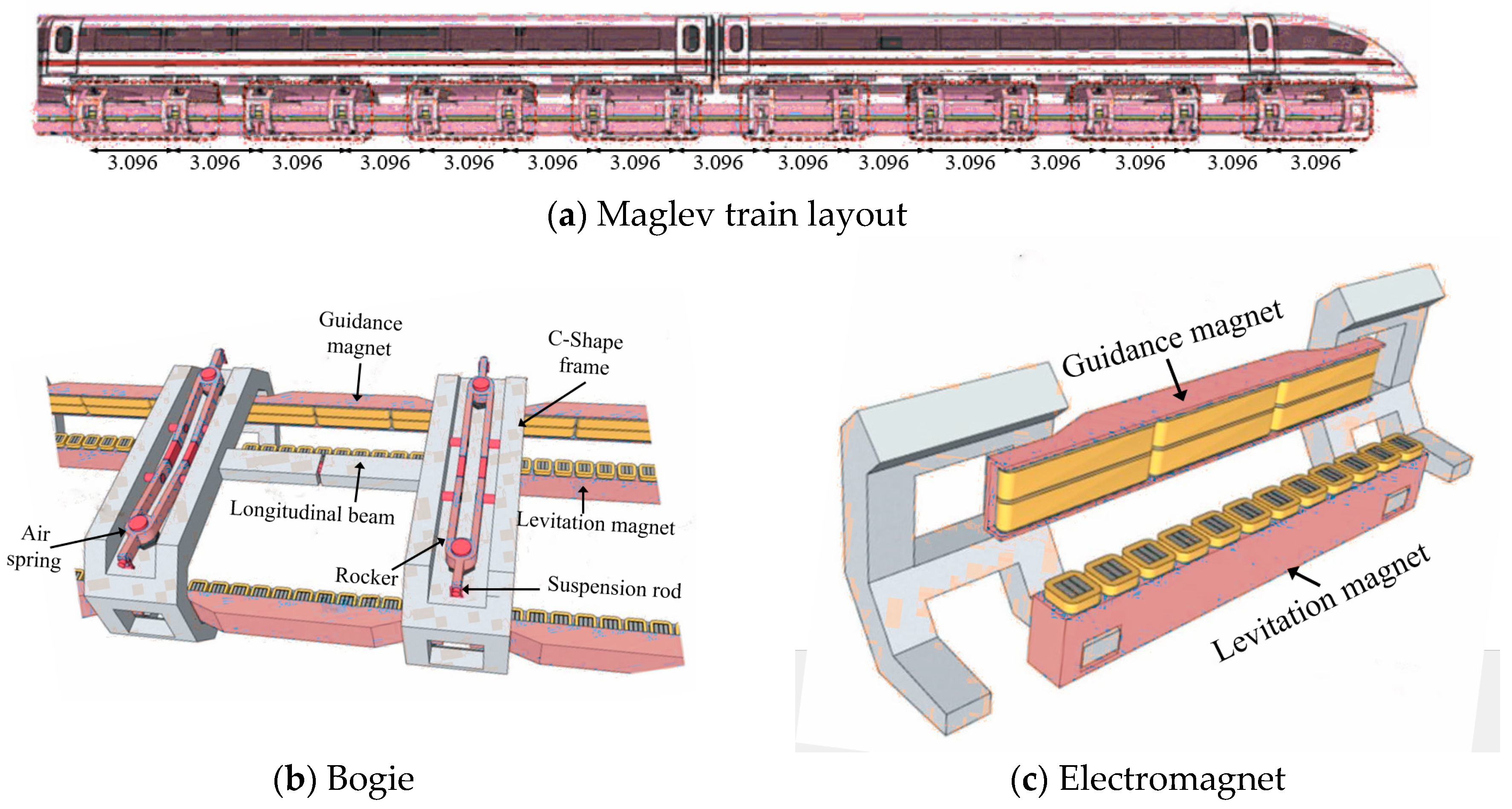
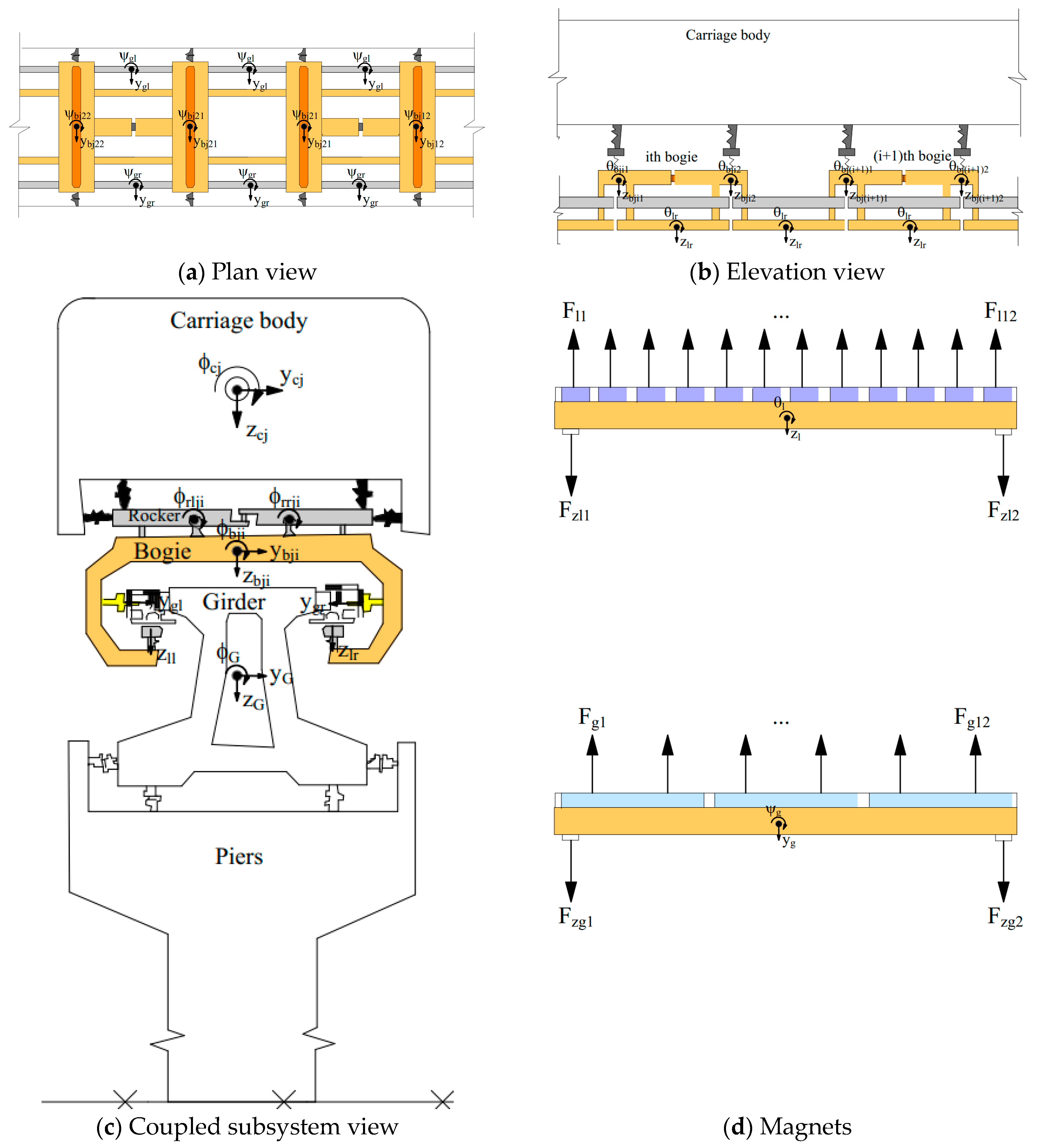
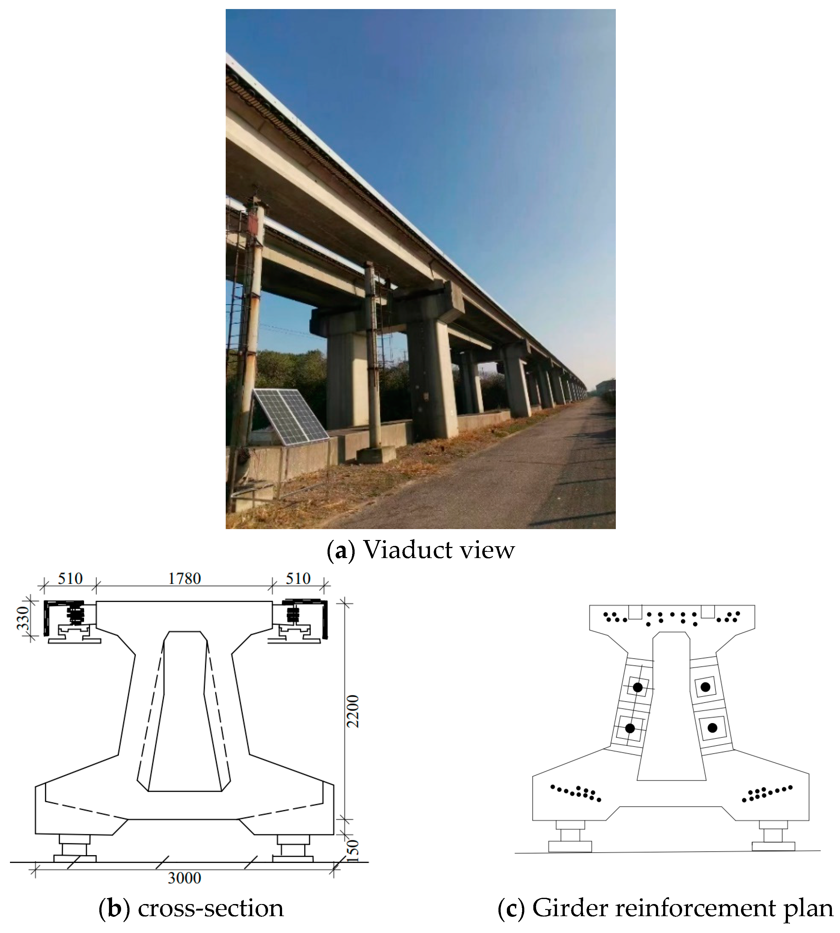
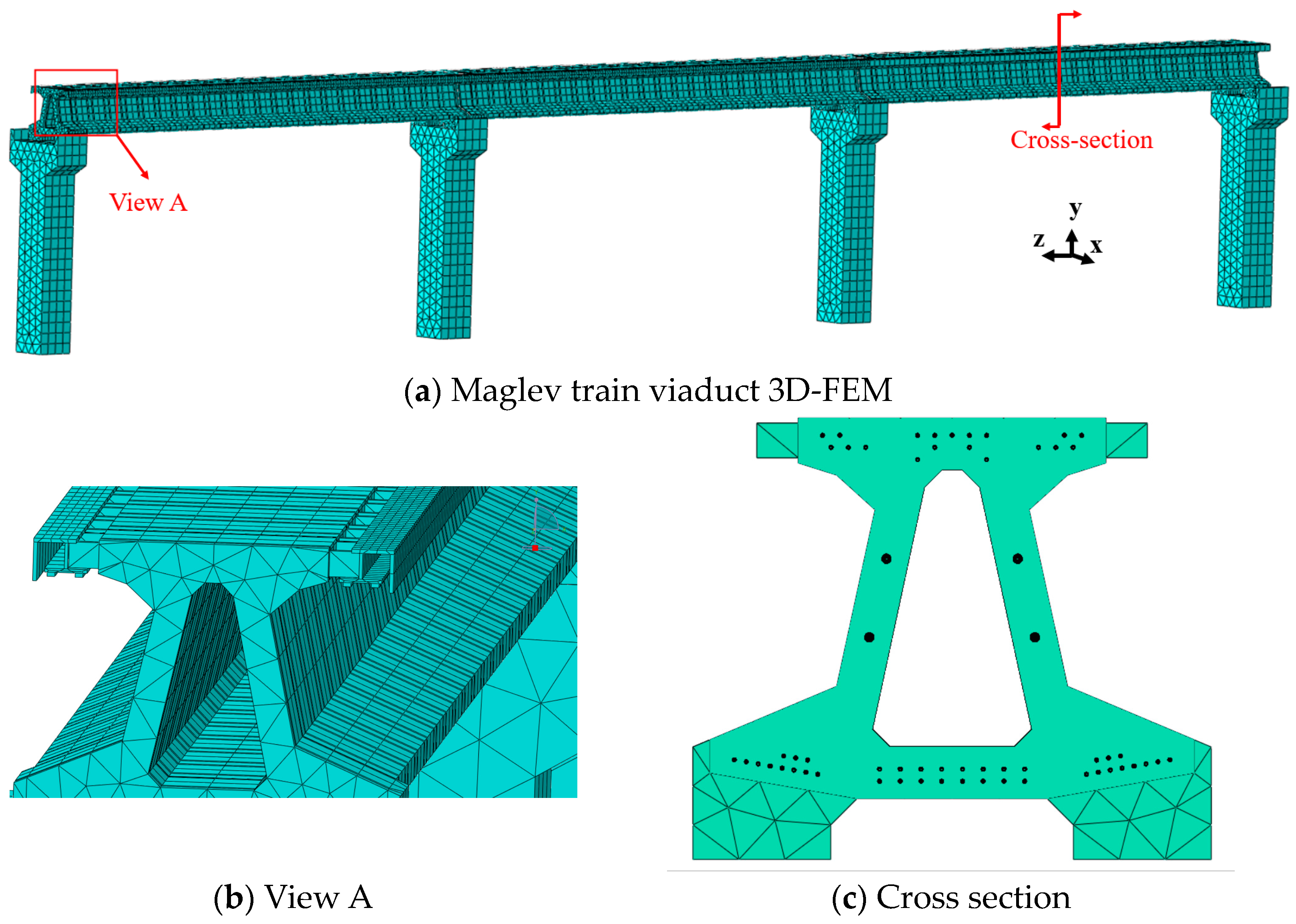
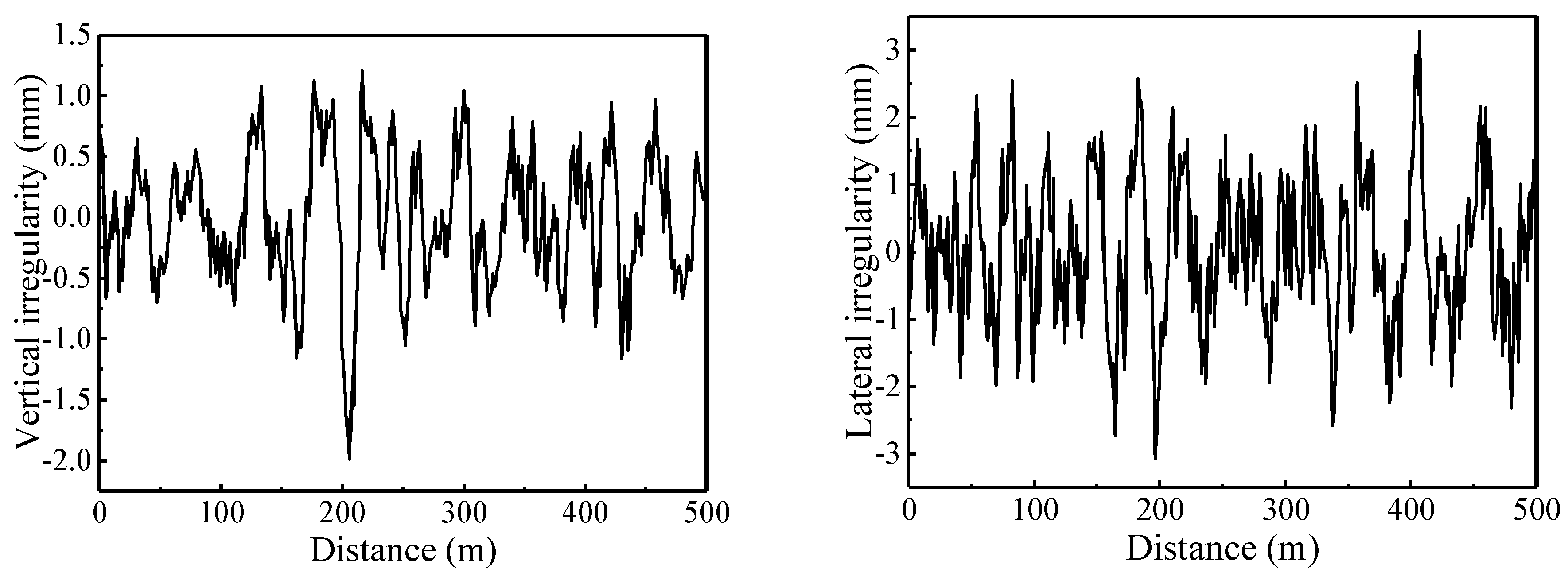
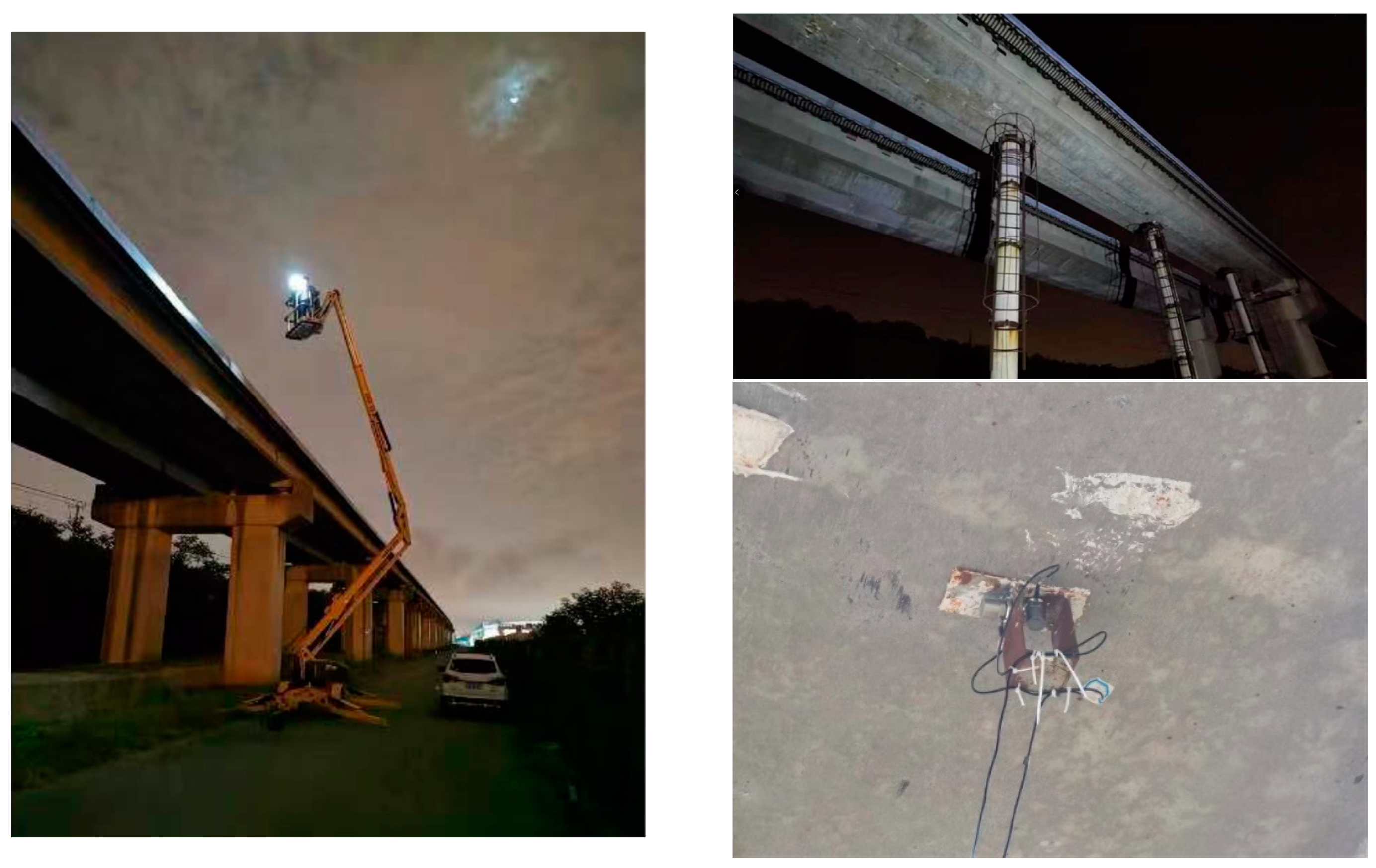
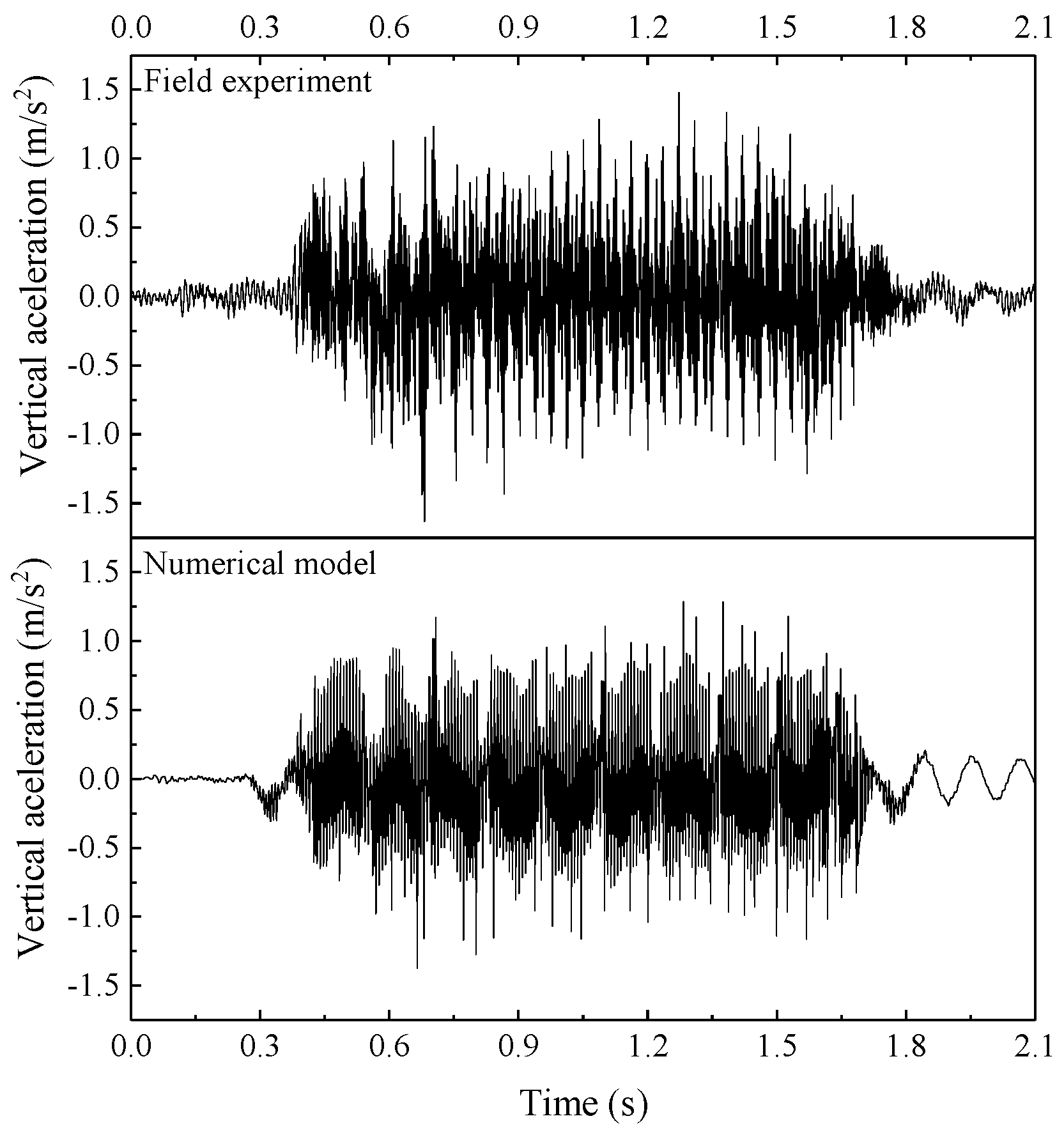
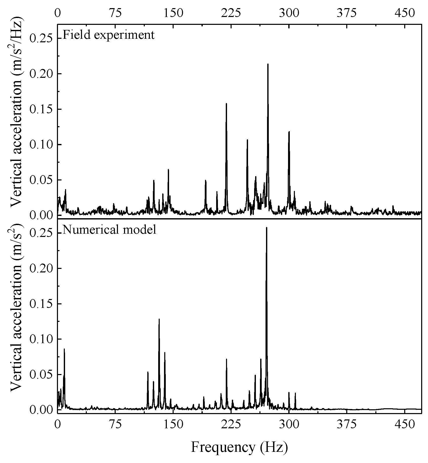
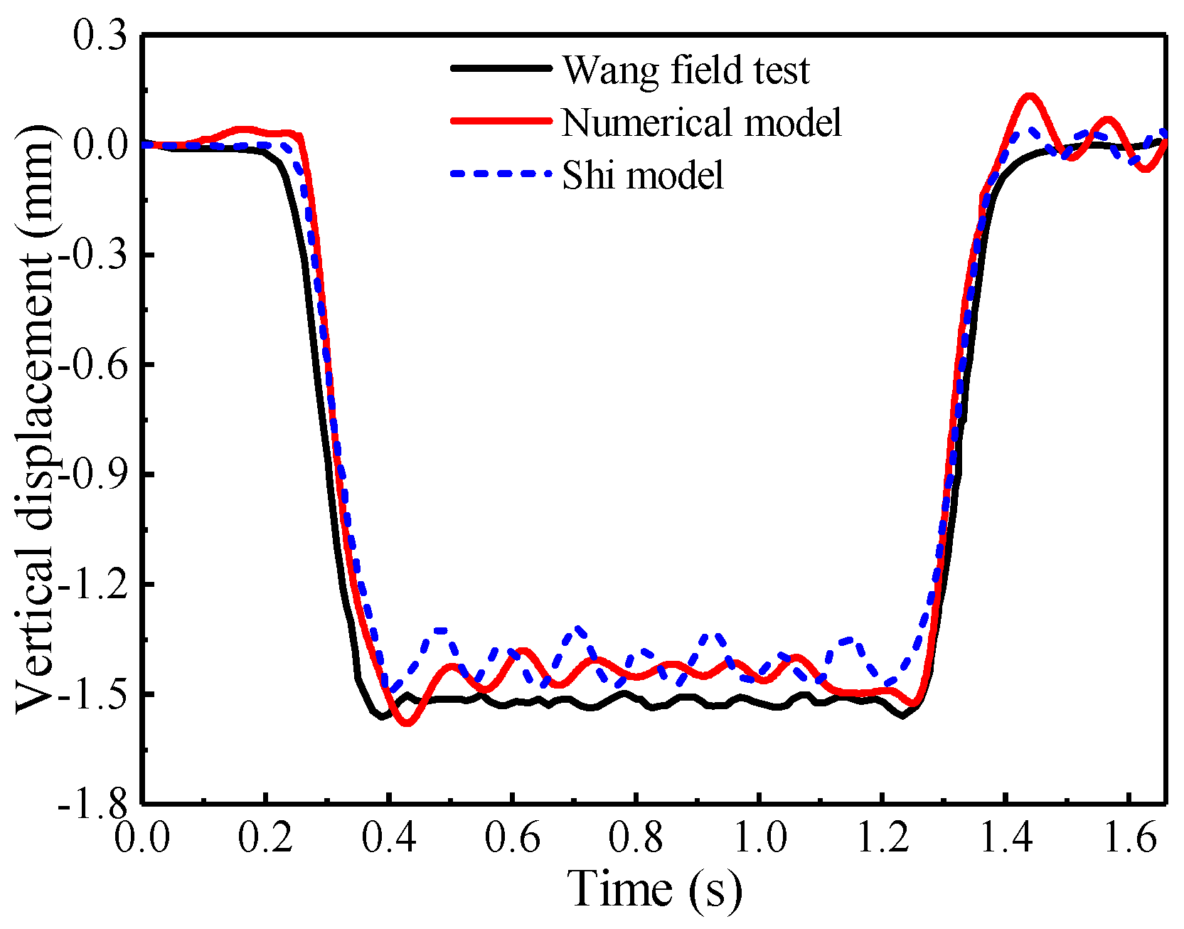
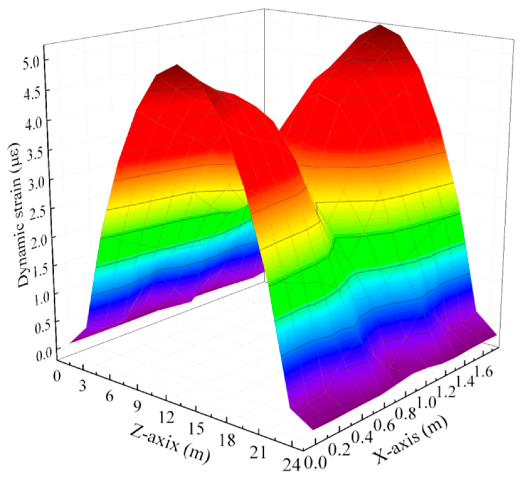
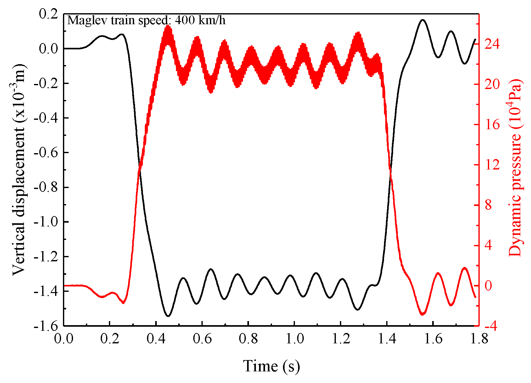
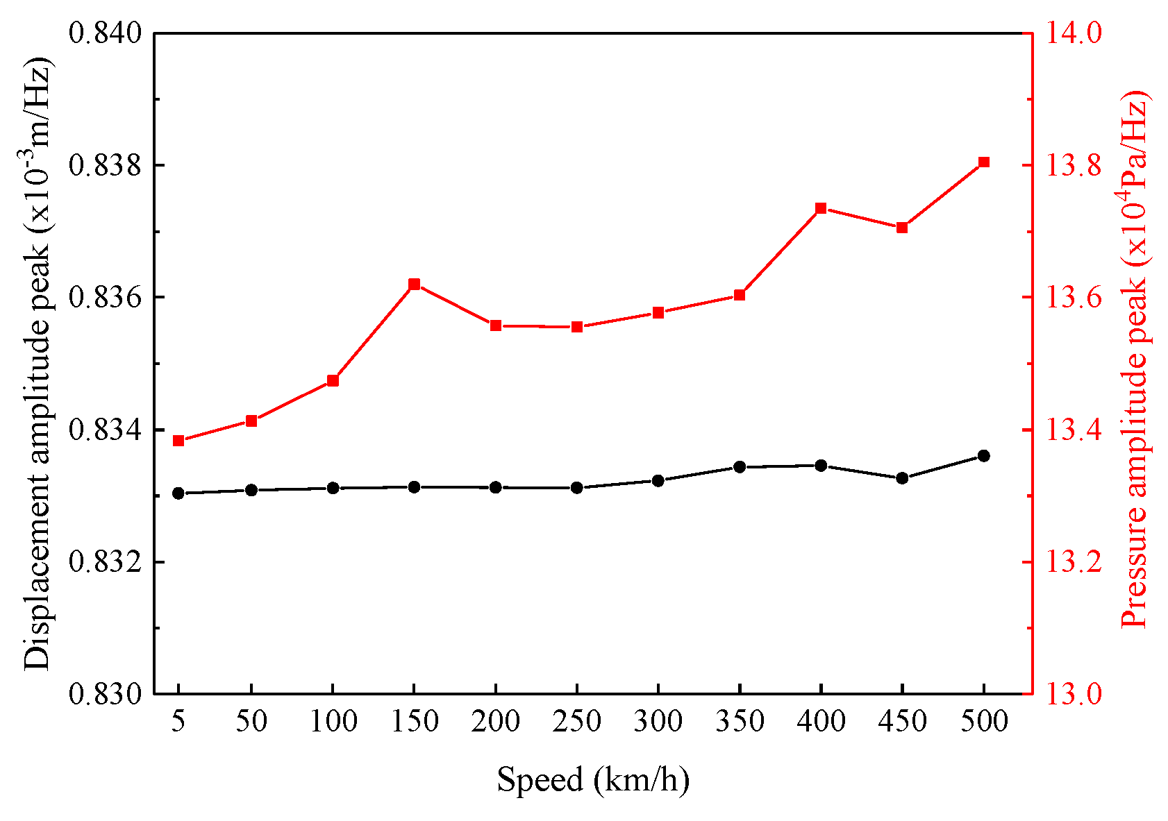
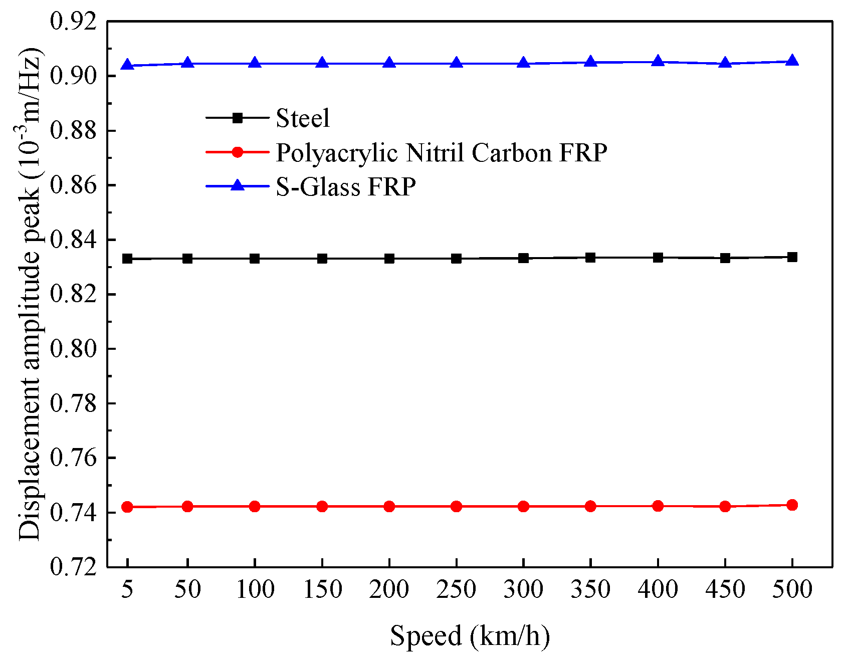


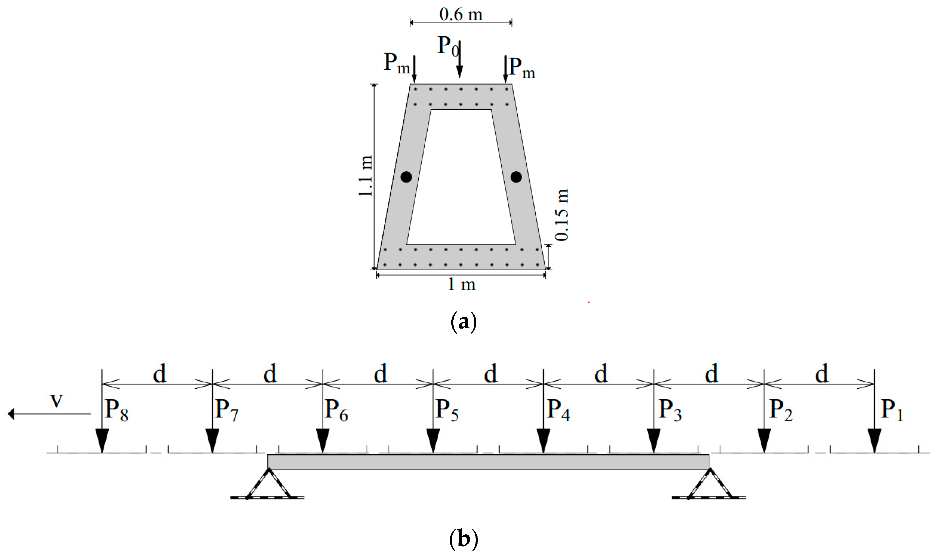
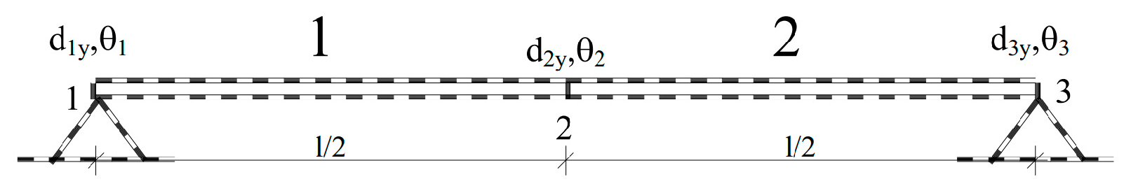

Disclaimer/Publisher’s Note: The statements, opinions and data contained in all publications are solely those of the individual author(s) and contributor(s) and not of MDPI and/or the editor(s). MDPI and/or the editor(s) disclaim responsibility for any injury to people or property resulting from any ideas, methods, instructions or products referred to in the content. |
© 2023 by the authors. Licensee MDPI, Basel, Switzerland. This article is an open access article distributed under the terms and conditions of the Creative Commons Attribution (CC BY) license (https://creativecommons.org/licenses/by/4.0/).