Autonomous Concrete Crack Semantic Segmentation Using Deep Fully Convolutional Encoder–Decoder Network in Concrete Structures Inspection

Abstract

Structure health inspection is the way to ensure that structures stay in optimum condition. Traditional inspection work has many disadvantages in dealing with the large workload despite using remote image-capturing devices. This research focuses on image-based concrete crack pattern recognition utilizing a deep convolutional neural network (DCNN) and an encoder–decoder module for semantic segmentation and classification tasks, thereby lightening the inspectors’ workload. To achieve this, a series of contrast experiments have been implemented. The results show that the proposed deep-learning network has competitive semantic segmentation accuracy (91.62%) and over-performs compared with other crack detection studies. This proposed advanced DCNN is split into multiple modules, including atrous convolution (AS), atrous spatial pyramid pooling (ASPP), a modified encoder–decoder module, and depthwise separable convolution (DSC). The advancement is that those modules are well-selected for this task and modified based on their characteristics and functions, exploiting their superiority to achieve robust and accurate detection globally. This application improved the overall performance of detection and can be implemented in industrial practices.

1. Introduction

A continuously increasing number of concrete structures worldwide are stepping into the ageing period. This could mean they are not in optimum operating condition, which will put the public at risk. According to the RAC Foundation’s investigation in 2019, the number of substandard road bridges has risen by 35% to 3203 in just two years in the UK [1]. Since the industrial revolution, thousands of bridges have been rapidly erected with the support of advanced engineering techniques and the demand for economic development. After decades of operation and exposure to wind and rain, these concrete structures’ upkeep has not been adequately monitored and confirmed with systematic evaluation. With fast-renewing technology, such as big data, artificial intelligence, and higher public property safety security requirements, a condition evaluation should meet the real-time monitoring and prediction for future conditions. Therefore, the risk of public property damage is lower while the surplus value remains stable. Thus, a novel way of efficient and accurate inspection is urgently needed to monitor a structure’s health condition.

A visual monitoring system controlled by cameras placed on the surface of concrete structures is an efficient way to monitor the condition of these structures [2]. However, it is not enough to improve the inspection only in the image-capturing stage. This process would still be time-consuming, with an overreliance on inspectors’ subjective assessments if cracks are recognized manually by humans. Hence, many studies on computer vision have been conducted on the classification or segmentation of image cracks.

The existing studies for crack classification, detection, and segmentation still contain optimization and detection issues. There is a little improvement regarding inspection methods used in practice relating to accuracy and efficiency. This research aims to improve the efficiency and accuracy of traditional concrete crack recognition by selecting, modifying, and assembling advanced convolution and pooling techniques and then validating them in repeated contrast experiments. To fully exploit their superiority, hyper-parameters are adjusted many times according to the changes in the repeated experiments’ results. In this research, the inference time of a crack is around 0.04 s per image on average, much faster than human recognition. The study focuses on the accuracy of crack recognition by building an advanced DCNN network. This paper does not discuss the parameter analysis that can be further reached by using this method.

The present paper first introduces vision-based defects detection and demonstrates deep fully convolutional neural network (DCNN) advancement compared to other methods in Section 2. Section 3 illustrates four applied modules that are used in this engineering application. Section 4 introduces raw crack image datasets that train the proposed network and manually labels 1650 images. Section 5 presents experiments and sets up the hyper-parameters for semantic segmentation and classification tasks. The results of the experiments are calculated and evaluated using several performance evaluation indicators in Section 6. The conclusion and future works are in Section 7.

2. Related Works

Performance, reliability, and safety are common concerns for in-service buildings and infrastructure. To ensure that these structures are sound, structure health monitoring (SHM) systems, which visually inspect structures, are often used to prevent structural failure in the early stages [3]. Today, advanced digital technologies have continuously been applied to support professionals in structure diagnosis activities. Koch et al. (2015) comprehensively reviewed the literature on state-of-art computer vision-based defect detection and condition assessment in concrete and asphalt civil infrastructure [4]. To date, machine learning and computer-vision-based methods have been widely applied in defect detection in the engineering field, such as vision-based techniques [5], machine vision-based techniques [6], machine learning, and deep learning-based approaches [7].

2.1. Computer Vision-Based Defect Detection in Engineering

Various vision-based methods have been studied to detect engineering defects, such as concrete cracks in buildings and other infrastructures. However, the collected images are hard to analyze and evaluate manually. To this end, Hutchinson et al. (2006) presented a statistical-based approach grounded in Bayesian decision theory for a work of image analysis that particularly aimed to assess concrete damages [8]. Ikhlas Abdel-Qader et al. (2003) illustrated an evaluation of four crack-detection techniques, including the fast Haar transform (FHT), fast Fourier transform (FFT). According to Sobel and Canny, FHT was found to be the most reliable method in identifying cracks [9]. Yu et al. (2007) realized complete crack detection using a semi-automatic algorithm called the Dijkstra method with Sobel and Laplacian operators’ help in finding crack edges [10]. Adhikari et al. (2013) proposed an integrated model using spectral analysis to develop the numerical representation of defects based on digital image processing to detect the development of cracks [11]. Prasanna et al. (2016) proposed a novel automatic crack-detection algorithm called the spatially tuned robust multi-feature (STRUM) classifier, which utilizes robust curve fitting to locate cracks and compute multiple visual features [12]. Dinh et al. (2016) developed an algorithm for automatically detecting significant peaks representing cracks from the grey-scale histogram representing the background and identifying the threshold value for image binarization [13]. To solve this problem of crack images being taken at a distance of more than one meter from the surface, Noh et al. (2017) proposed a segmentation method via fuzzy C-means clustering to detect a crack [14]. Sato et al. (2018) proposed a V-shaped detector for detecting cracks of 0.2 mm or less [15]. Ali et al. (2018) modified the cascade face detection technique based on the Viola–Jones algorithm to see cracks with bounding boxes [16].

2.2. Vision-Based Methods

However, most vision-based methods are manually designed to extract crack features. These methods usually lack accuracy and efficiency. Since there is an increasing number of visual inspections requiring non-contacting crack detection and recognition, machine vision-based methods provide a more efficient and accurate way of detecting cracks. To achieve a higher level of automated inspection, Oh et al. (2009) implemented a robotic inspection system consisting of a customized truck, a robot with a mobility control system, and a machine vision system for detecting cracks [17]. Zou et al. (2012) proposed CrackTree, a fully automatic method for detecting pavement cracks from images, sequentially using a geodesic shadow-removal algorithm, tensor voting for a building crack probability map, and a graph model representing crack seeds from the crack probability map [18]. Chambon and Moliard (2011) illustrated a fine-defect detection based on a multi-scale extraction and Markovian segmentation in pavement surfaces [19]. Instead of using a handcrafted feature extractor, Ebrahimkhanlou et al. (2015) applied multi-fractal analysis (MFA) to automatically extract information hidden behind crack patterns taken from reinforced concrete shear walls [20]. Many efforts have been made to help prevent non-uniform illumination and contamination using image processing techniques to enhance crack recognition accuracy. To extract cracks more effectively and robustly, Ying and Salari (2010) applied a pavement distress picture enhancement algorithm to eliminate the background lighting variation or correct the non-uniform background light distribution, followed with a Beamlet transform-based approach that automatically detects pavement cracks [21].

Nevertheless, with the emphasis on eliminating and correcting illuminance conditions, the increased complexity of procedures leads to higher computation costs. Valença et al. (2011) introduced an innovative method called “MCRACK”, which combined digital image processing and mathematical morphology (MM) for the automatic detection and monitoring of cracks [22]. This technique using non-professional cameras has a low computational cost and allows for a non-contract robust measurement. Tsai et al. (2013) illustrated how the crack map was developed and used for the crack path planning process based on a so-called geodesic minimal path-based method [23]. As the size of images has continuously increased, which requires a significant amount of computation time, Yamaguchi and Hashimoto (2009) demonstrated an efficient high-speed crack-recognition method that utilizes proposed termination, skip-added procedures, and percolation-based image processing [24]. Therefore, image-processing techniques have been used widely in the last decade to detect cracks in concrete walls, bridges, pavements, and underground pipelines.

2.3. Machine Vision Methods

Based on various crack-detection experiment results, it is impossible to eliminate all forms of noise in high-contrast light distribution, contamination, lumps, and holes on the concrete surface by handcrafting the features. As a result, artificial intelligence and machine learning have been widely used in crack detection with either supervised or unsupervised training for crack detection and noise elimination. Regarding automatic crack extraction in concrete bridge decks, the trend of the crack detection methods is moving to machine learning-based cracks or noise features extraction from handcraft feature extraction (Table 1). The reason for this trend is the convenience and accuracy of machine-learning methods, which could efficiently and automatically extract the information behind both crack and various noise features.

Table 1. Computer vision-based defect detection in engineering.

Article	Description	Advantages and Disadvantages
Ikhlas Abdel-Qader et al. (2006) [25]	(1) experimented with three different principal component analyses (PCAs) implemented directly on the raw data in a global framework, (2) practiced PCA on the data to enhance the result after linear features were detected, and (3) practiced PCA with the feature detected only on the segmented small individual block of the data.	The automatic crack extraction method was used to identify concrete cracks in the early stage; the accuracy is low. Linear patterns may be identified as cracks, the anti-interference ability is weak, and the operation is complicated.
Choudhary and Dey (2012) [26]	Presented fuzzy logic and artificial neural network (ANN)-based models to extract crack features from digital images, including (1) an images approach which classifies an image globally and (2) an object approach which classifies cracks and noise locally in an image.	Uses ANN in the early stage of image-based crack feature extraction; can classify the image only if there is a crack or noise; accuracy is low; the speed and accuracy are low since the convolutional layer is not used in the neural network in this stage.
Na and Tao (2012) [27]	Provided an approach for pavement surface image classification using a proximal support vector machine (PSVM), which is easier to manipulate than the traditional support vector machine (SVM).	Easier to operate than SVM; it is suitable for binary classification problems but challenging to handle image tasks with a large amount of data; the speed is slower than that of the convolutional neural network.
Li et al. (2017) [28]	Developed a fully automatic machine-learning algorithm to extract cracks with the assistance of a proposed feature selection method based on a linear SVM with a wide-ranging search strategy for noise elimination.	Uses noise elimination and SVM-based novel feature selection; both were used to improve crack recognition accuracy. The method is complicated and cannot perform pixel-wise semantic segmentation tasks.
Kim et al. (2018) [29]	Proposed a machine-learning approach for the use of classifying cracks and noise patterns by (1) applying image binarization for extracting crack candidate regions and (2) classifying images using trained classification models, which are built based on speeded-up robust features and convolution neural network (CNN).	Built up a good foundation for DCNN application in crack detection; recognition speed and accuracy are relatively low; has limited application in pixel-wise semantic segmentation tasks.
Dai et al. (2019) [30]	Implemented a novel methodology applying the genetically optimized online sequential extreme learning machine. This machine utilizes sequential learning algorithms that do not require retraining once new data are uploaded. It also features bootstrap confidence intervals for predicting the behaviour of a concrete crack in a dam.	This method has good generalization performance and a fast learning speed, but the image classification task is only suitable for real-time computing scenarios and cannot perform pixel-wise semantic segmentation tasks; accuracy is relatively low

However, the performance of the existing shallow machine-learning algorithms is often unsatisfactory. This is because shallow machine-learning algorithms cannot extract high-level features, leading to the omission of critical information behind noise features in terms of crack-like stains, lumps, and holes in the training process. For this reason, machine-learning algorithms for crack detection must perform better and be capable of deeper analysis. Zhang et al. (2018) trained a deep convolutional neural network (DCNN) to classify pavement images into the crack, sealed crack, and background categories and then applied tensor voting-based curve detection to detect cracks and sealed cracks [31]. Inspired by the region proposal network’s success (RPN), which is used for fast R-CNN detection, Ren et al. [28] introduced. In 2016, Cha et al. (2018) utilized a deep machine-learning model called the faster region-based convolutional neural network (Faster R-CNN) that trained on a database containing 2366 labelled images (with 500 × 375 pixels) to classify 5 types of structural damages [32]. Chen and Jahanshahi (2018) proposed a deep-learning framework to identify cracks in individual video frames based on a CNN and a naïve Bayes data fusion scheme named NB-CNN [33]. Tao et al. (2018) introduced a dual procedure that could accurately classify and localize metallic defects in pictures captured from actual industrial environments [34]. This study uses a novel cascaded autoencoder (CASAE) architecture to transform input pictures with defects into a pixel-level prediction mask and then employs a compact convolutional neural network for various defect classification types. Recently, Xu et al. (2019) proposed an end-to-end crack classification network based on DCNN, which applies the advances of atrous convolution, an atrous spatial pyramid pooling (ASPP) module, and depthwise separable convolution [35]. As professional camera devices are expensive and too inconvenient for image data collecting, the smartphone camera has performed satisfactorily in these tasks in recent years. Maeda et al. (2018) created a publicly available database containing 9053 road damage images captured by a smartphone with 15,435 instances of road surface damage in various road surface finishes, weather, and illuminance conditions and annotated the location and type of damages using bounding boxes [36]. Inspired by the success of applying deep learning in computer vision, Zhang et al. (2016) trained a supervised DCNN on a dataset of 500 images (with 3264 × 2448 pixels) collected by a low-cost smartphone. In recent years, with the popularity of transfer learning used in computer vision [37], for example, Gopalakrishnan et al. (2017) achieved acceptable results through employing a DCNN by transferring the features trained from ImageNet, which contains millions of images, to automatically detect cracks in hot-mix asphalt (HMA) and Portland cement concrete (PCC) [38]. Since then, transfer learning has been widely applied in various examples of deep learning-based computer vision to enhance the accuracy and efficiency of damage detection.

Most deep learning-based computer vision techniques use bounding boxes to label crack patterns during training and to detect crack patterns in the test process. Whereas the crack pattern usually consists of thin, vague dark strips or lines with continuously varying angles and directions, they cannot be accurately marked using bounding boxes. To address these limitations, Dung and Anh (2018) and Islam and Kim (2019) successfully proposed a fully convolutional network (FCN) with an encoder–decoder architecture for crack pattern recognition and segmentation using VGGNet as the encoder’s backbone [39].

The above studies achieved decent results in crack classification, detection, and segmentation, but there are no significant developments in optimization and detection accuracy of classification and segmentation. In this research, a state-of-the-art FCN-based technique is proposed to classify images into crack or non-crack and to detect cracks by segmenting them from a background on a pixel-wise level. Furthermore, this network could be used directly in industrial practices to reduce the inspectors’ workloads and improve inspection speed dramatically.

The present study proposes a DCNN-based method for concrete crack recognition and segmentation. First, the whole encoder–decoder network containing different DCNN backbones is trained to end for semantic segmentation on an annotated image dataset to find the best-performing network depth. The most accurate DCNN backbone is then used to classify the images in the same publicly available dataset as the inspection routine requirement is image-wise. Finally, the proposed network’s overall performance is validated using crack and non-crack images collected from bridges. This method is innovative because the noises, such as crack-like stains, lumps, and holes in raw images, do not need to be eliminated, and each targeted crack is marked at a pixel-wise level. However, this method could not be used for detecting cracks caused by carbonation phenomena and corrosion, etc., except for stress.

3. Research Methods

This study proposes various methods to optimize existing convolution operation, pooling operation, information context extraction, and recovery to improve automatic crack detection performance. After several optimization iterations, four modules crucial to achieving competitive segmentation performance in this study are chosen for detailed illustration. The composition of these four modules allows for the following: (1) the neural network to go deeper; (2) a dramatic decrease in the number of parameters; (3) thin, weakened dark crack strips or lines with continuously varying angles and directions can be marked at a pixel-wise level instead of using bounding boxes; and (4) enhanced accuracy of crack detection. Standard performance evaluation methods measure the effectiveness of these modules. This section demonstrates the modules and experiment steps (Figure 1) of proposed method used in the proposed network below.

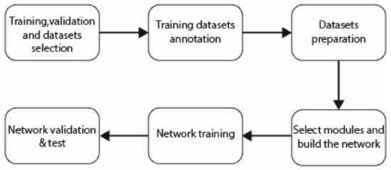
Figure 1. The steps of the proposed method.

3.1. Atrous Convolution

Traditional object detection consolidates multi-scale context information in images by using continuous pooling layers responsible for the loss of detailed information and the degradation of image resolution [40]. A novel method called atrous convolution (or so-called dilated convolution) was proposed to overcome this problem. This operation can also exponentially enlarge the receptive field with much less resolution loss [41].

3.2. Atrous Spatial Pyramid Pooling (ASPP)

In DCNN, the extent of context information utilized is determined by the size of the receptive field. In practice, the empirical receptive field is much smaller than the theoretical receptive field [42]. To solve this problem, the global average pooling shows proven efficiency in obtaining global context information. However, global average pooling may cause a loss of sub-region context information. In 2015, He et al. created a spatial pyramid pooling (SPP) process to collect multi-scale information, improving efficiency and accuracy. In terms of bridges, cracks often appear in a small region of images [43]. Thus, to accurately identify crack features, the atrous convolution is integrated with SPP (known as atrous spatial pyramid pooling; ASPP) to avoid the loss of detailed context information during a sub-sampling operation. The ASPP achieves parallel atrous sampling on a given input feature map with different rates and fuses, thereby obtaining multi-scale context information of an image.

3.3. Encoder–Decoder Structure

The encoder–decoder network has been effectively utilized in various visual works, including object detection and semantic segmentation. Usually, an encoder–decoder architecture comprises the following: (1) an encoder section that gradually decreases the dimension of feature maps and extracts higher feature context; and (2) a decoder section that recovers low-level feature information by enlarging the dimension of the feature maps [44].

3.4. Depthwise Separable Convolution

Laurent Sifre first introduced the depthwise separable convolution in 2014 [45]. It was widely used in many advanced deep-learning models, such as Xception. The most significant advantage of depthwise separable convolution compared to standard convolution is a dramatic decrease in the parameters and computation complexity while achieving slightly better performance. The depthwise separable convolution is a standard convolution layer decomposed into a depthwise convolution followed by a pointwise convolution.

Based on the four modules, this study first utilized an encoder module to decrease input images’ dimension and extract higher feature context. In the encoder section, the Xception models (Figure 2) serve as the encoder’s backbone, using atrous convolution and depthwise separable convolution in each layer to save computation time and expense. Atrous spatial pyramid pooling (ASPP) is also applied during the encoder process to enlarge the empirical receptive field for a more effective gathering of global context information. Secondly, the decoder section gradually recovers the low-level feature information and concatenates this with high-level feature information by enlarging the feature maps’ dimensions. To assess these assembled modules’ performance, train loss is used to monitor learning efficiency, while the confusion matrix and related indicators reflect accuracy.

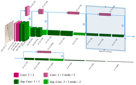
Figure 2. The structure of the used Xception model in this study.

4. Datasets for Semantic Segmentation and Classification

4.1. Training and Validation Datasets for Semantic Segmentation

To train a robust crack detection network, these datasets includes images with various shading, strains, and illuminance that are referenced by the publicly extant concrete cracks datasets [35,46]. Specifically, (1) 224 × 224 pixels from 6069 crack images collected from bridges by a Phantom 4 Pro’s CMOS cameras by Xu et al. (2019) [35] and (2) 227 × 227 pixels from 40,000 crack images collected at a stock of campus buildings of the Middle East University by Özgenel (2019) are used for training testing and validation. All high-resolution pictures are captured with the device about 30–50 cm from the concrete structure. The pictures have high surface finishes and illumination condition variance to avoid the impact of concrete surface finishes and illumination conditions. In this study, network training and validation images are randomly selected from the one shared by Özgenel (2019) [46], which contains essential cracks more suitable for network training and validation, as shown in Table 2. For network training, the dataset contains two image formats, as follows: (1) jpg images are raw images (24-bit RGB images), and (2) png images are annotated images (8-bit grey map). The training dataset contains 1000 crack images and 500 background images. For validation, the dataset includes 100 crack images and 50 background images. Therefore, there are two classifications, namely crack and background.

Table 2. Training and validation datasets for semantic segmentation.

	No. of Crack Images	No. of Non-Crack Images	No. of Jpg Images	No. of Png Images
Train dataset	1000	500	1500	1500
Validation dataset	100	50	150	150

4.2. Test Datasets for Semantic Segmentation and Classification

To test the selected crack detection networks’ performance in classifying cracks by segmenting the cracks from background, two datasets (Table 3) are generated from the two publicly available datasets mentioned in Chapter 4.1. Since the training and validation datasets are generated from the database shared by Özgenel (2019) [46], images in the first test dataset (containing 1000 crack images and 500 background images) are randomly selected from their parent dataset to test their performance on the same dataset. To ensure generalization ability, the networks are also tested on a selection from the second dataset, whose images are randomly selected from the dataset shared by Zhang et al. (2017), containing 1000 crack images and 500 non-crack images [31].

Table 3. Datasets for testing.

	No. of Crack Images	No. of Non-Crack Images	Author
Train dataset	1000	500	Çağlar Fırat Özgenel [46]
Validation dataset	100	50	Xu et al. [35]

5. Experiment

This study uses semantic segmentation to indicate the crack’s path and density based on each pixel’s prediction. Model performance was first compared based on the percentage of correct predictions on a pixel-wise level (semantic segmentation task) to ensure accurate results. Because the crack and non-crack pixel classification enhance the detailed classification performance of a set of selected models, the most suitable models will be used for classification tasks on two different datasets, in order to test whether the network is robust and has generalization ability, respectively. This study applies an encoder–decoder, a fully convolutional network with end-to-end learning. A series of experiments are proposed to test the highest prediction accuracy by deepening the encoder’s backbone. Three deep-learning models, namely Xception_41, Xception_65, and Xception_71, are used to analyze the model’s accuracy and depth. Note that 41, 65, and 71 are the number of layers (the so-called depth) of the models. All experiments proposed in this study were performed on an Intel(R) Core(T.M.) i7-8750H CPU@ 2.20 GHz CPU with 16GB RAM and a NVIDIA GTX1060 GPU, Cardiff, Wales. For the convenience of building and implementing the network, the convolutional neural network was constructed using the Slim module within TensorFlow, an open-source deep-learning project developed by Google.

5.1. Preparation

5.1.1. Image Selection from Parent Datasets

As mentioned in Table 2, to generate the training dataset and validation dataset as a whole, 1100 images with crack features are scheduled to be randomly selected from the 20,000-image crack-positive parent dataset; meanwhile, 550 non-crack images are randomly selected from the 20,000-image crack-negative parent dataset. A Python script was written to realize efficient random crack image selection and rename each image chosen in the order of 1–1100. Non-crack images are also randomly selected and ordered from 1101 to 1650. Ordering these images makes it easier to match the raw images with labelled images. Therefore, raw images with cracks and backgrounds are sufficiently prepared and ordered following the annotation process.

5.1.2. Crack and Background Annotation

Lanbelme, written in Python, was used to annotate cracks and backgrounds in the prepared raw images. The labelling crack and background interfaces are shown in Figure 3, where (a) is the interface of crack annotation. The crack crosses the image from top to bottom and is circled by the polygon, which consists of many green lines and is marked with an index of “crack.” In Figure 3b, the entire image region is circled using a rectangle and marked as “background.” This indicates the circled pixels in the image as crack pixels or so-called positive pixels. The circled positive pixels are also known as ground truth, which provides the correct classification for calculating train loss and instructing training and validation. The annotation information is added to the corresponding image and generated in a .json format. Finally, 1100 crack images and 550 background images were annotated and put in the .json format.

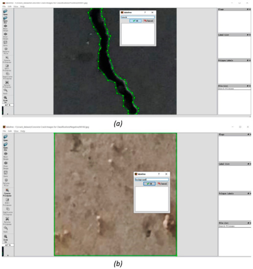
Figure 3. Crack (a) and background (b) annotation interfaces.

5.1.3. Pre-Processing of Annotated Images

Next, the raw images and .json files are conjointly transformed into an 8-bit colour map according to the label name index. The crack paths and density are correspondingly marked in red. A Python script is written to automatically transform images into a colour map and visualize each class marked in the annotation process.

Each pixel’s colour value in images is reset according to the classes annotated. After the Python script operation, the output has four different types of files, as follows: (1) raw image, (2) npy files storing segmentation class, (3) colour map with marked red crack path and density, and (4) class visualization images. The colour map marked with a red crack path and density is shown in Figure 4; the class visualization images are shown in Figure 5.

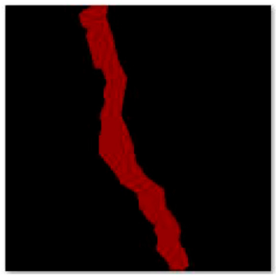
Figure 4. The 8-bit colour map with marked crack path and density.

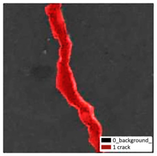
Figure 5. Class visualization image.

5.1.4. Storing Image Data into Binary Record

As the data is streamed over the network during training and validation, storing the image data in a binary record sequence is the best option. Therefore, all the training and validation images are recorded on a set of .tfrecord format files according to the training dataset and validation dataset’s preset index. Tfrecord is a type of binary data storing format using a protocol buffer for data encoding. The foremost reason for transforming thousands of images into a TFrecord is that reading the data over different disk areas before putting it into memory is too time-consuming and impractical. However, pre-transforming the data into a binary data format and putting it into a continuous buffer dramatically increased processing speed. The data from 1500 training images are divided into 5 .tfrecord files; correspondingly, the data from 150 validation images are divided into 5 .tfrecord files.

5.2. Pre-Trained Models for Semantic Segmentation

For more efficient training performance, transfer learning is applied in this study. The selected Xception models are first trained on ImageNet, an enormous human-annotated image database containing 14,197,122 images. The model’s structure and parameters (weights and bias) are recorded at the start of this crack feature learning task.

The training pipeline of DeepLabV3+ is used for this crack segmentation task (Figure 6). Image data are first imported into the DCNN module (encoder’s backbone), specifically the Xception models in the encoder module. In Xception models, the images are streamed sequentially through the entry, middle, and exit flow. The structure of the Xception model containing 65 layers only consists of standard convolutions and depthwise separable convolutions. The Xception model used here differs from the original Xception model in each block’s last operation. For Xception_41, the middle flow repeats eight times. For Xception_65 and Xception_71, the middle flow repeats 8 and 16 times, respectively. Compared to the original Xception model proposed by Chollet (2017) [47], the max pooling operation and global average pooling in the Xception model in this study are all replaced by separable convolutions to reduce the computation complexity. Secondly, the ASPP module with different rates (6, 12, and 18) of atrous convolution probes the output features from the DCNN module at multiple scales for robust object segmentation.

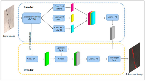
Figure 6. The architecture of DeepLabv3+ in this study.

In the decoder module, the encoder’s crack features are first binary up-sampled by a factor =4 and then combined with correspondingly linked low-level features with the same number of channels and the same spatial dimension from the encoder’s 53 backbone. To decrease the number of channels, 1 × 1 convolution is applied on each corresponding low-level feature to reduce their channels, as shown in Figure 6. Secondly, another binary up-sampling with a factor = 4 is applied following a few 3 × 3 convolutions for refining the features.

In this study, the Xception_65 was first utilized as the encoder’s backbone to find the highest mean intersection over union (mIOU) by applying many refinements. The refinements are mainly implemented by adjusting the hyper-parameters (Table 4). Batch size is related to the computation speed. Parameter 2 is used due to limited computational power. Furthermore, 100 is the point where the training loss remains almost constant. Other hyper-parameters are also tested to prove the most suitable settings. The settings in Table 4 are to test the accuracy results of different layers. As such, this decides which type of Xception model we use as the backbone for the network. Furthermore, the refinement with the best performance is taken as the baseline training procedure. Next, the same refinement was applied to adjust the other two Xception models’ hyper-parameters, namely Xception_41 and Xception_71. Therefore, comparing models based on the same refinements, hardware, and encoder–decoder architecture is fair. Note that the semantic segmentation performance is evaluated using the value of mIOU generated from the validation procedure.

Table 4. The hyper-parameter settings for training and validation.

Hyper-Parameters/Models	Xception_41	Xception_65	Xception_71
No. of layers	41	65	71
Batch size	2	2	2
No. of epochs	100	100	100
Base learning rate	0.001	0.001	0.001
Learning rate decay factor	0.1	0.1	0.1
Learning rate decay step	2000	2000	2000
Atrous rate for ASPP	[6,12,18]	[6,12,18]	[6,12,18]
Decoder up-sample factors	[4,4]	[4,4]	[4,4]

5.3. Pre-Trained Models for Classification

In most practical cases, the crack inspection work distinguishes whether cracks are in an image. Thus, segmenting the crack pixels semantically from its background is unnecessary, and could waste computation resources. According to the calculated mIOU in the validation process, the best-performing model will be utilized to classify crack and background images in datasets 1 and 2. The weights and biases recorded during training will then be stored as checkpoint files (.ckpt format) for inference. However, the checkpoint files only contain the model’s parameters and not the structure of the model itself. Thus, the recorded key and value of parameters have to be matched with the model’s structure in a single .pb file using an API called tf. train from the Tensorflow framework, as shown in Figure 7.

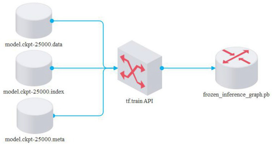
Figure 7. Combination of model structure, key, and value of parameters.

The structured model with key and value parameters was then used as the backbone for predicting cracks in the two test datasets, namely dataset 1 and dataset 2. In this phase, the cracks will be segmented from the background, but the mIOU of each dataset will not be calculated. Because the images in test datasets do not have semantic annotation, the mIOU (the mean accuracy of correctly predicted pixels) cannot be calculated. Thus, this is not an evaluation indicator for classification.

6. Results and Discussions

6.1. Network Performance Evaluation

Several widely used evaluation methods for both classification and semantic segmentation tasks are utilized to quantitatively assess the performance of the models used in this research.

6.1.1. Train Loss

To monitor the learning process’s progress, train loss represents the distance between annotated cracks and predicted cracks. Train loss is a critical indicator showing whether or not the training dataset has been sufficiently learned. Over time, this indicator becomes an essential factor in deciding whether to stop or continue the learning process.

The calculation of train loss is cross-entropy. In Equation (1) below, for cross-entropy, the H(p,q) represents the probability error between two probability distributions, p and q, while k p and k q are the real and non-real distributions, respectively. In Equation (2) shown below, for train loss, k, y is true to label distributions, representing the corresponding annotated classes, such as crack and background in this study, while k S represent predicted crack and background distributions, respectively, which are values of probability output from softmax.

$$H\left(p,q\right)={{\displaystyle \sum }}_{k=1}^N{p}_k {log}_2\frac{1}{p_k}$$

(1)

$$Loss=-{{\displaystyle \sum }}_{k=1}^N{y}_k log S_k$$

(2)

6.1.2. Confusion Matrix

The confusion matrix is mainly used to evaluate the performance of classification and semantic segmentation tasks. In Figure 8, the confusion matrix contains the following four items: (1) true positive, (2) false positive, (3) false negative, and (4) true negative. The four items are performed on image instances in the classification task, while the four items are also on pixel instances in semantic segmentation tasks. The four items are presented as follows:

(1)

The T.P. (true positive) defines the number of positive inspections predicted to be positive. In this study, T.P. represents the number of crack images in classification or crack pixels in semantic segmentation tasks correctly classified as crack image or pixel instances;

(2)

The T.N. (true negative) defines the number of negative inspections predicted to be negative. In this study, T.N. represents the number of background images in classification or background pixels in semantic segmentation tasks that are correctly classified as background image instances or background pixel instances;

(3)

The F.P. (false positive) defines the number of negative inspections predicted to be positive. In this study, F.P. represents the number of background images in classification or background pixels in semantic segmentation tasks incorrectly classified as crack images or pixel instances;

(4)

The F.N. (false negative) defines the number of positive inspections predicted to be negative. In this study, F.N. represents the number of crack images in classification or crack pixels in semantic segmentation tasks incorrectly classified as background image or background pixel instances.

Figure 8. Confusion matrix of crack and non-crack.

6.1.3. Evaluation Factors

Several evaluation factors are calculated using the identified results from the mentioned confusion matrix. The evaluation factors are listed as follows:

Mean intersection of union (mIOU) is the percentage of correctly predicted positive pixels to the total number of true positive pixels and the negative pixels incorrectly predicted as positive pixels, as shown in Equation (3). The mIOU in this study refers to the percentage of correctly predicted crack pixel instances in all true crack pixel instances and incorrectly predicted crack pixel instances.

$$mIOU=\frac{TP}{FP+FN+TP}$$

(3)

Accuracy is the percentage of the number of correctly classified image instances to the total number of image instances, as shown in Equation (4). Accuracy in this study refers to the percentage of correctly classified crack and background images.

$$Accuracy=\frac{TP+TN}{TP+TN+FP+FN}$$

(4)

Precision is the percentage of the number of true positive instances to the number of all positive predictions, as shown in Equation (5). Precision in this study refers to the percentage of the true crack images in all image instances predicted as cracks.

$$Precision=\frac{TP}{TP+FP}$$

(5)

Sensitivity (recall) is the percentage of the number of positive instances that correctly classified the number of all true positive image instances, as shown in Equation (6). Sensitivity in this study refers to the percentage of the correctly identified positive image instances in all true positive image instances.

$$Sensitivity=\frac{TP}{TP+FN}$$

(6)

Specificity is the percentage of the number of negative instances that correctly identified the number of all negative instances, as shown in Equation (7). Specificity in this study refers to the ratio of correctly classified background image instances in all true background image instances.

$$Specificity=\frac{TN}{TN+FP}$$

(7)

F1-Score is calculated when the value F measures the distance between positive and predicted labels in a dataset by the classifier, as shown in Equation (9). The F1-Score refers to the distance between labelled and predicted cracks in this study, as shown in Equation (9). Note that the parameter α is equal to 1 in this study, and the higher the F1-Score is, the more efficient the model is.

$$F=\frac{\left({\alpha }^2+1\right)Precision\times Sensitivity}{{\alpha }^2\left(Precision+Sensitivity\right)}$$

(8)

$$F_1=\frac{2\times Precision\times Sensitivity}{\left(Precision+Sensitivity\right)}$$

(9)

6.2. Crack Images for Semantic Segmentation

For training, the selected three models that serve as the encoder’s backbone are trained for 100 epochs (Table 4) using 1000 crack images and 500 non-crack images (Table 2) that are randomly selected from the concrete crack dataset shared by Özgenel (2019) [46]. Figure 9 shows the training loss of three networks with different depths of Xception models that employed the cross-entropy loss function as the objective function against the number of steps. The blue line represents the train loss trend of Xception 41, which has 41 layers. The yellow line represents the train loss trend of Xception 65 with 65 layers, while the red line represents the train loss trend of Xception 71 with 71 layers. From the result, no matter which Xception model of the three we discuss, it is evident that with the increased number of epochs, the train loss value decreases dramatically until approximately 10,000 steps. Although there are several fluctuations from 10,000 steps to the end of the training (75,000 steps), the train loss value shows a slightly downward trend from above 0.4 to below 0.4.

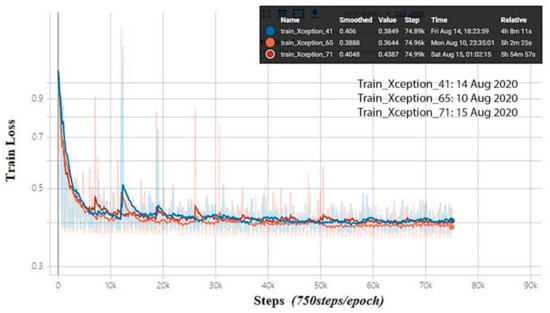
Figure 9. The training loss of Xception_71 during training.

For validation, the already-trained three models that serve as the encoder’s backbone are successively used to predict the validation dataset containing 100 crack images and 50 background images (Table 2). The predicted crack images and non-crack images are shown in Figure 10. As shown in Figure 10a, the input image (left) is a 227 × 227 pixels raw image, the segmentation map (middle) is the predicted image with red pixels representing crack pixels, and the segmentation overlay (right) is the overlay of raw image and translucent segmentation map. There are no red pixels in Figure 10b, just as there are no crack pixels in the raw image.

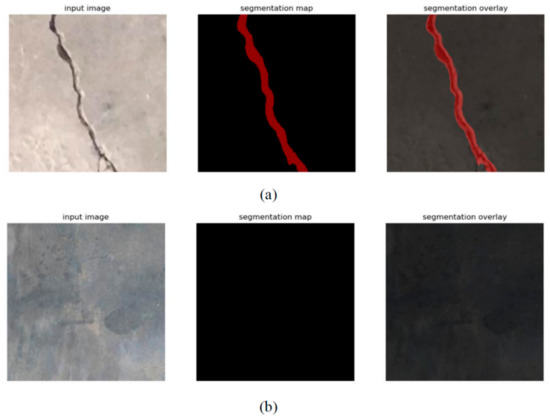
Figure 10. Validation results of crack images (a) and background images (b).

The most widely used evaluation indicator is mIOU for semantic segmentation tasks. The mIOUs of the network, with three different encoder backbones, are shown in Table 5. It is clear that with the increasing depth of the model, the mIOU is higher, having the same 100 learning epochs. The overall mIOU is the average value of background mIOU and crack mIOU. Consequently, the Xception_71 model is selected for the following 61 crack classification tasks.

Table 5. The mIOUs of the selected three models.

	mIOU of Background	mIOU of Crack	Overall mIOU	No. of Epochs
Xception_41	0.986364901	0.843513668	0.914939284	100
Xception_65	0.986514747	0.844588637	0.915551662	100
Xception_71	0.986991405	0.849419773	0.918205619	100

To view the performance of this combination of encoder backbone model and network, the results of Xception_71 are compared to a recent study by Dung and Anh (2019) [39] in terms of accuracy in Table 6. The proposed network in this study using the Xception 71 model has higher average accuracy than Dung and Anh’s network, while the highest accuracy is just slightly lower than the network proposed by Dung and Anh. The comparison indicates that the proposed network is highly competitive but has room for improvement.

Table 6. Performance comparison of this study and Dung and Anh’s study.

Network	Average Accuracy	Highest Accuracy
Performance of this study	91.62%	91.82%
Dung and Anh’s network	90.9%	91.9%

6.3. Crack Images for Classification during the Test

When the network has a satisfactory performance during validation, it is then tested on two datasets, namely sub-datasets of its parent dataset and another publicly available concrete crack dataset shared by Xu et al. (2019) [35].

6.3.1. Test on the Parent Dataset: Dataset 1

The network with the most accurate model, Xception_71, is predicted on dataset 1, randomly selected from the same training and validation dataset. It achieved quite a huge success in concrete crack classification task. As the confusion matrix shows in Figure 11a, there was 100% accuracy in all evaluation indicators (Table 7) on dataset 1. Three more datasets (1a, 1b, and 1c) are generated with randomly selected crack and background images from the same parent dataset containing 40,000 images to avoid contingency. The test accuracy of the three sub-datasets is shown in Table 7.

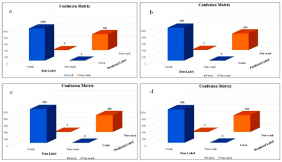
Figure 11. The confusion matrix of Xception_71 test on the test dataset 1 (a), 1a (b), 1b (c), and 1c (d).

Table 7. The evaluation indicators tested on different datasets.

Dataset	Accuracy	Precision	Sensitivity (Recall)	Specificity	F1-Score
Dataset 1	100%	100%	100%	100%	1.0
Dataset 1a	99.86%	100%	99.8%	100%	0.999
Dataset 1b	99.93%	100%	99.9%	100%	1.0
Dataset 1c	99.86%	100%	99.8%	100%	0.999

6.3.2. Test on Another Different Source Dataset: Dataset 2

As dataset 1 is generated from the same training and validation dataset, the generalization ability may not be properly tested on dataset 1. Therefore, dataset 2 is generated from another publicly available dataset containing 6069 images. Because of the different concrete surface finishes and types of crack, this network’s performance is less competitive, as its confusion matrix shows in Figure 12. Furthermore, the corresponding evaluation results are shown in Table 8. Although the implementation of this network is less competitive on dataset 2, it still outperformed most of the current studies (Table 9) in concrete crack classification, such as SVM [48], CNN [32], FCN proposed by Manjurul Islam and Kim [49], and the encoder–decoder network using a model proposed by Xu et al. (2019) [35].

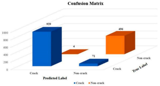
Figure 12. The confusion matrix of the Xception_71 test on the test dataset 2.

Table 8. The evaluation indicators tested on dataset 2.

	Accuracy	Precision	Sensitivity (Recall)	Specificity	F1-Score
Dataset 2	95%	95.57%	92.90%	99.20%	0.9612

Table 9. A comparison of several methods on image classification.

Model/Network	Accuracy	Precision	Sensitivity	Specificity	F1-Score
SVM	71.87%	68.75%	73.33%	-	0.7096
CNN	81.87%	88.75%	78.02%	-	0.8304
FCN	92.8%	91.3%	94.1%	-	0.8304
Model by Xu et al.	96.37%	78.11%	100%	95.83%	0.8771
Proposed network	95%	99.57%	92.9%	99.2%	0.9612

7. Conclusions and Future Work

This study reviews the history of automatic defect recognition and implements the DCNN method as the most accurate and efficient way for concrete structure crack detection. The technical operation modules used in DCNN are introduced. The preparation of a set of datasets and a series of experiments are presented. The performance evaluation methods for semantic segmentation and classification are demonstrated to compare this proposed network with other existing networks. The results show that this proposed network’s performance was satisfactory regarding concrete crack recognition compared to other studies. The proposed method indicates that it can accurately detect and highlight the crack boundary. Futhermore, it can reduce the inspectors’ workload by offering intuitive and fast operation. Therefore, it is a valuable application for inspecting bridges or other types of infrastructure.

This study’s original contribution to the literature is that it applied a set of Xception models, including a residual network and depthwise separable convolution as the encoder’s backbone in an encoder–decoder network that contained an ASPP module for automatic concrete crack recognition. The proposed method exploits each module’s superiority in characteristics and functionality and innovatively optimizes the results by integrating different networks. Therefore, this method shows satisfactory performance in terms of efficiency and accuracy.

As introduced in this study, more detailed information, such as the crack dimension, location, and importance of the crack components, is needed for rating structure health conditions. However, the current methods cannot structure the images according to their location for the convenience of retracing. Future work could focus on matching an image with its dimensions location and how to retrace the importance of the component. For example, the UAV should capture an image with its location saved using the Global Positioning System (GPS) or the Big Dipper Coordinate System (BDCS). Next, the location could be stored in a digital twin (DT) model using building information modelling (BIM) and used to locate each component for its importance checking and visualized overall rating.

References

- RAC Foundation. More than 3000 GB Road Bridges Are Substandard. 2017. Available online: https://www.racfoundation.org/media-centre/spanning-the-gap-road-bridge-maintenance-in-britain (accessed on 1 September 2020).
- Ahanshahi, M.R.; Masri, S.F.; Sukhatme, G.S. Multi-image stitching and scene reconstruction for evaluating defect evolution in structures. Struct. Health Monit. 2011, 10, 643–657. [Google Scholar] [CrossRef]
- Pallarés, F.J.; Betti, M.; Bartoli, G.; Pallarés, L. Structural health monitoring (SHM) and Nondestructive testing (NDT) of slender masonry structures: A practical review. Constr. Build. Mater. 2021, 297, 123768. [Google Scholar] [CrossRef]
- Koch, C.; Georgieva, K.; Kasireddy, V.; Akinci, B.; Fieguth, P. A review on computer vision based defect detection and condition assessment of concrete and asphalt civil infrastructure. Adv. Eng. Inform. 2015, 29, 196–210. [Google Scholar] [CrossRef]
- Mordia, R.; Kumar Verma, A. Visual techniques for defects detection in steel products: A comparative study. Eng. Fail. Anal. 2022, 134, 106047. [Google Scholar] [CrossRef]
- Eshkevari, M.; Jahangoshai Rezaee, M.; Zarinbal, M.; Izadbakhsh, H. Automatic dimensional defect detection for glass vials based on machine vision: A heuristic segmentation method. J. Manuf. Process. 2021, 68, 973–989. [Google Scholar] [CrossRef]
- Wang, W.; Su, C.; Fu, D. Automatic detection of defects in concrete structures based on deep learning. Structures 2022, 43, 192–199. [Google Scholar] [CrossRef]
- Hutchinson, T.C.; Chen, Z. Improved Image Analysis for Evaluating Concrete Damage. J. Comput. Civ. Eng. 2006, 20, 210–216. [Google Scholar] [CrossRef]
- Abdel-Qader, I.; Abudayyeh, O.; Kelly, M.E. Analysis of Edge-Detection Techniques for Crack Identification in Bridges. J. Comput. Civ. Eng. 2003, 17, 255–263. [Google Scholar] [CrossRef]
- Yu, S.-N.; Jang, J.-H.; Han, C.-S. Auto inspection system using a mobile robot for detecting concrete cracks in a tunnel. Autom. Constr. 2007, 16, 255–261. [Google Scholar] [CrossRef]
- Adhikari, R.S.; Moselhi, O.; Bagchi, A. Image-based retrieval of concrete crack properties for bridge inspection. Autom. Constr. 2014, 39, 180–194. [Google Scholar] [CrossRef]
- Prasanna, P.; Dana, K.J.; Gucunski, N.; Basily, B.B.; La, H.M.; Lim, R.S.; Parvardeh, H. Automated Crack Detection on Concrete Bridges. IEEE Trans. Autom. Sci. Eng. 2016, 13, 591–599. [Google Scholar] [CrossRef]
- Dinh, T.H.; Ha, Q.P.; La, H.M. Computer vision-based method for concrete crack detection. In Proceedings of the 2016 14th International Conference on Control, Automation, Robotics and Vision (ICARCV), Phuket, Thailand, 13–15 November 2016; pp. 1–6. [Google Scholar] [CrossRef]
- Noh, Y.; Koo, D.; Kang, Y.-M.; Park, D.; Lee, D. Automatic crack detection on concrete images using segmentation via fuzzy C-means clustering. In Proceedings of the 2017 International Conference on Applied System Innovation (ICASI), Sapporo, Japan, 13–17 May 2017; pp. 877–880. [Google Scholar] [CrossRef]
- Sato, Y.; Bao, Y.; Koya, Y. Crack Detection on Concrete Surfaces Using V-shaped Features. World Comput. Sci. Inf. Technol. 2018, 8, 1–6. [Google Scholar]
- Cha, Y.-J.; Lokekere Gopal, D.; Ali, R. Vision-based concrete crack detection technique using cascade features. In Sensors and Smart Structures Technologies for Civil, Mechanical, and Aerospace Systems 2018; SPIE: Bellingham, WA, USA, 2018; p. 21. [Google Scholar] [CrossRef]
- Oh, J.-K.; Jang, G.; Oh, S.; Lee, J.H.; Yi, B.-J.; Moon, Y.S.; Lee, J.S.; Choi, Y. Bridge inspection robot system with machine vision. Autom. Constr. 2009, 18, 929–941. [Google Scholar] [CrossRef]
- Zou, Q.; Cao, Y.; Li, Q.; Mao, Q.; Wang, S. CrackTree: Automatic crack detection from pavement images. Pattern Recognit. Lett. 2012, 33, 227–238. [Google Scholar] [CrossRef]
- Chambon, S.; Moliard, J.-M. Automatic Road Pavement Assessment with Image Processing: Review and Comparison. Int. J. Geophys. 2011, 2011, 1–20. [Google Scholar] [CrossRef]
- Ebrahimkhanlou, A.; Farhidzadeh, A.; Salamone, S. Multifractal analysis of two-dimensional images for damage assessment of reinforced concrete structures. In Sensors and Smart Structures Technologies for Civil, Mechanical, and Aerospace Systems 2015; SPIE: Bellingham, WA, USA, 2015; p. 94351A. [Google Scholar] [CrossRef]
- Ying, L.; Salari, E. Beamlet Transform-Based Technique for Pavement Crack Detection and Classification. Comput. Aided Civ. Infrastruct. Eng. 2010, 25, 572–580. [Google Scholar] [CrossRef]
- Valença, J.; Dias-da-Costa, D.; Júlio, E.N.B.S. Characterization of concrete cracking during laboratorial tests using image processing. Constr. Build. Mater. 2012, 28, 607–615. [Google Scholar] [CrossRef]
- Tsai, Y.; Kaul, V.; Yezzi, A. Automating the crack map detection process for machine operated crack sealer. Autom. Constr. 2013, 31, 10–18. [Google Scholar] [CrossRef]
- Yamaguchi, T.; Hashimoto, S. Fast crack detection method for large-size concrete surface images using percolation-based image processing. Mach. Vis. Appl. 2010, 21, 797–809. [Google Scholar] [CrossRef]
- Abdel-Qader, I.; Pashaie-Rad, S.; Abudayyeh, O.; Yehia, S. PCA-Based algorithm for unsupervised bridge crack detection. Adv. Eng. Softw. 2006, 37, 771–778. [Google Scholar] [CrossRef]
- Choudhary, G.K.; Dey, S. Crack detection in concrete surfaces using image processing, fuzzy logic, and neural networks. In Proceedings of the 2012 IEEE Fifth International Conference on Advanced Computational Intelligence (ICACI), Najing, China, 18–20 October 2012; pp. 404–411. [Google Scholar] [CrossRef]
- Na, W.; Tao, W. Proximal support vector machine based pavement image classification. In Proceedings of the 2012 IEEE Fifth International Conference on Advanced Computational Intelligence (ICACI), Najing, China, 18–20 October 2012; pp. 686–688. [Google Scholar] [CrossRef]
- Li, G.; Zhao, X.; Du, K.; Ru, F.; Zhang, Y. Recognition and evaluation of bridge cracks with modified active contour model and greedy search-based support vector machine. Autom. Constr. 2017, 78, 51–61. [Google Scholar] [CrossRef]
- Kim, H.; Ahn, E.; Shin, M.; Sim, S.-H. Crack and Noncrack Classification from Concrete Surface Images Using Machine Learning. Struct. Health Monit. 2019, 18, 725–738. [Google Scholar] [CrossRef]
- Dai, B.; Gu, C.; Zhao, E.; Zhu, K.; Cao, W.; Qin, X. Improved online sequential extreme learning machine for identifying crack behavior in concrete dam. Adv. Struct. Eng. 2019, 22, 402–412. [Google Scholar] [CrossRef]
- Zhang, K.; Cheng, H.D.; Zhang, B. Unified Approach to Pavement Crack and Sealed Crack Detection Using Preclassification Based on Transfer Learning. J. Comput. Civ. Eng. 2018, 32, 04018001. [Google Scholar] [CrossRef]
- Cha, Y.-J.; Choi, W.; Suh, G.; Mahmoudkhani, S.; Büyüköztürk, O. Autonomous Structural Visual Inspection Using Region-Based Deep Learning for Detecting Multiple Damage Types. Comput. Aided Civ. Infrastruct. Eng. 2018, 33, 731–747. [Google Scholar] [CrossRef]
- Chen, F.-C.; Jahanshahi, M.R. NB-CNN: Deep Learning-Based Crack Detection Using Convolutional Neural Network and Naïve Bayes Data Fusion. IEEE Trans. Ind. Electron. 2018, 65, 4392–4400. [Google Scholar] [CrossRef]
- Tao, X.; Zhang, D.; Ma, W.; Liu, X.; Xu, D. Automatic Metallic Surface Defect Detection and Recognition with Convolutional Neural Networks. Appl. Sci. 2018, 8, 1575. [Google Scholar] [CrossRef]
- Xu, H.; Su, X.; Wang, Y.; Cai, H.; Cui, K.; Chen, X. Automatic Bridge Crack Detection Using a Convolutional Neural Network. Appl. Sci. 2019, 9, 2867. [Google Scholar] [CrossRef]
- Maeda, H.; Sekimoto, Y.; Seto, T.; Kashiyama, T.; Omata, H. Road Damage Detection and Classification Using Deep Neural Networks with Smartphone Images. Comput. Aided Civ. Infrastruct. Eng. 2018, 33, 1127–1141. [Google Scholar] [CrossRef]
- Zhang, L.; Yang, F.; Zhang, Y.D.; Zhu, Y.J. Road crack detection using deep convolutional neural network. In Proceedings of the 2016 IEEE International Conference on Image Processing (ICIP), Phoenix, AZ, USA, 25–28 September 2016; pp. 3708–3712. [Google Scholar] [CrossRef]
- Gopalakrishnan, K.; Khaitan, S.K.; Choudhary, A.; Agrawal, A. Deep Convolutional Neural Networks with transfer learning for computer vision-based data-driven pavement distress detection. Constr. Build. Mater. 2017, 157, 322–330. [Google Scholar] [CrossRef]
- Dung, C.V.; Anh, L.D. Autonomous concrete crack detection using deep fully convolutional neural network. Autom. Constr. 2019, 99, 52–58. [Google Scholar] [CrossRef]
- Simonyan, K.; Zisserman, A. Very Deep Convolutional Networks for Large-Scale Image Recognition. arXiv 2014, arXiv:1409.1556. [Google Scholar]
- Yu, F.; Koltun, V. Multi-Scale Context Aggregation by Dilated Convolutions. arXiv 2015, arXiv:1511.07122. [Google Scholar]
- Zhou, B.; Khosla, A.; Lapedriza, A.; Oliva, A.; Torralba, A. Object Detectors Emerge in Deep Scene CNNs. arXiv 2014, arXiv:1412.6856. [Google Scholar]
- He, K.; Zhang, X.; Ren, S.; Sun, J. Spatial Pyramid Pooling in Deep Convolutional Networks for Visual Recognition. IEEE Trans. Pattern Anal. Mach. Intell. 2015, 37, 1904–1916. [Google Scholar] [CrossRef]
- Chen, L.-C.; Zhu, Y.; Papandreou, G.; Schroff, F.; Adam, H. Encoder-Decoder with Atrous Separable Convolution for Semantic Image Segmentation. arXiv 2018, arXiv:1409.1556. [Google Scholar]
- Vanhoucke, V. Learning visual representations at scale. arXiv 2014, arXiv:2006.06666. [Google Scholar]
- Özgenel, Ç.F. Concrete Crack Images for Classification; Version 2; Mendeley Data; Orta Dogu Teknik Universitesi: Ankara, Turkey, 2019. [Google Scholar] [CrossRef]
- Chollet, F. Xception: Deep Learning with Depthwise Separable Convolutions. arXiv 2016, arXiv:1610.02357. [Google Scholar]
- Yeum, C.M.; Dyke, S.J. Vision-Based Automated Crack Detection for Bridge Inspection. Comput. Aided Civ. Infrastruct. Eng. 2015, 30, 759–770. [Google Scholar] [CrossRef]
- Islam, M.M.M.; Kim, J.-M. Vision-Based Autonomous Crack Detection of Concrete Structures Using a Fully Convolutional Encoder–Decoder Network. Sensors 2019, 19, 4251. [Google Scholar] [CrossRef]
Publisher’s Note: MDPI stays neutral with regard to jurisdictional claims in published maps and institutional affiliations. |
© 2022 by the authors. Licensee MDPI, Basel, Switzerland. This article is an open access article distributed under the terms and conditions of the Creative Commons Attribution (CC BY) license (https://creativecommons.org/licenses/by/4.0/).