Article

Correlation between Ground Motion Parameters and Displacement Demands of Mid-Rise RC Buildings on Soft Soils Considering Soil-Structure-Interaction

Department of Civil Engineering, Pamukkale University, 20160 Denizli, Turkey
*
Author to whom correspondence should be addressed.
Buildings 2021, 11(3), 125; https://doi.org/10.3390/buildings11030125
Submission received: 3 February 2021 / Revised: 5 March 2021 / Accepted: 15 March 2021 / Published: 19 March 2021
(This article belongs to the Section Building Structures)

Abstract

:
This paper investigates the correlation between ground motion parameters and displacement demands of mid-rise RC frame buildings on soft soils considering the soil-structure interaction. The mid-rise RC buildings are represented by using 5, 8, 10, 13, and 15-storey frame building models with no structural irregularity. A total of 105 3D nonlinear time history analyses were carried out for 21 acceleration records and 5 different building models. The roof drift ratio (RDR) obtained as inelastic displacement demands at roof level normalized by the building height is used for demand measure, while 20 ground motion parameters were used as intensity measure. The outcomes show velocity related parameters such as Housner Intensity (HI), Root Mean Square of Velocity (Vrms), Velocity Spectrum Intensity (VSI) and Peak Ground Velocity (PGV), which reflect inelastic displacement demands of mid-rise buildings as a damage indicator on soft soil deposit reasonably well. HI is the leading parameter with the strongest correlation. However, acceleration and displacement related parameters exhibit poor correlation. This study proposed new combined multiple ground motion parameter equations to reflect the damage potential better than a single ground motion parameter. The use of combined multiple parameters can be effective in determining seismic damages by improving the scatter by at least 24% compared to the use of a single parameter.

1. Introduction

The seismic hazard is quantified by the intensity measure (peak ground values of acceleration (PGA), velocity (PGV), etc.) of a ground motion, while the structural damage state is defined by the demand measures (maximum interstorey and roof drift ratio, etc.) [1]. Many relationships between Intensity Measure (IM) and Demand Measure (DM) for performance-based earthquake engineering (PBEE) researches have been presented in the literature [2,3,4,5,6,7,8,9]. The damage potential of structures was reflected by the ground motion parameters (GMP) such as Peak Ground Acceleration (PGA), Peak Ground Velocity (PGV), Peak Ground Displacement (PGD), etc. Although PGA has been used as a dominant parameter in structural and earthquake engineering research, some studies have shown that this parameter provides a poor correlation for the representation of structural damage [10,11,12]. The potential damage of the structure depends on the energy and frequency content, the number of cycles, density and duration, etc. of the ground motion record [13,14]. It is very important for PBEE to obtain a ground motion parameter, which represents the statistical relationship between IM and DM with smaller dispersions [1]. For this reason, many studies are ongoing on the issue of the GMP, to reflect the statistically best structural damage potential.
Elenas and Meskouris [15] examined the relation between maximum interstorey drift ratio/overall structural damage index of a 7-storey reinforced concrete (RC) frame building and 10 different GMPs using 20 acceleration records. The authors emphasized that spectral and energy parameters exhibit good correlation, while peak ground motion parameters have a weak correlation. Nanos et al. [16] expanded the study using 450 different artificial seismic records. The results showed that a medium correlation was obtained between the damage index of the 6-storey RC frame building and the PGA, while a strong correlation was observed with Arias Intensity (Ia).
Cao and Ranogh [17] investigated the correlation between 23 different GMPs with the interstorey drift ratio and damage index of the 3-storey RC building. 1040 records were selected from 4 different earthquakes, which are far-fault motion. They concluded that Velocity Spectrum Intensity (VSI) has the best correlation, followed by Housner Intensity (HI) and Spectral Acceleration (Sa). Moreover, the low correlation observed for the PGA supported the other studies. Kostinakis and Athanatopolou [18] examined the correlation between spectral acceleration with an interstorey drift ratio of 3 symmetric and 3 asymmetric 5-storey buildings. It has been emphasized that the spectral acceleration (Sa) is a good indicator of the structural damage for mid-rise RC buildings with small eccentricity.
Yakut and Yilmaz [19] have used 16 RC frames and 80 ground motion records to investigate the correlation between the maximum interstorey drift and GMPs. They indicated that Housner Intensity (HI), VSI, and Acceleration Spectrum Intensity (ASI) have the strongest correlation for the period range of 0.1−2.5 s. PGA, VSI, and Characteristic Intensity (Ic) have the best parameters for the period range of 0.2−0.5 s, while VSI, HI, and Spectral Acceleration (Sa) are the best correlated parameters for the period range of 0.5−1.1.
In the studies summarized above, many Multi-Degree-of-Freedom (MDOF) systems with different numbers of floors were used. In addition, the relationships between structural damage potential and GMPs were examined on Single-Degree-of-Freedom (SDOF) systems. Akkar and Ozen [1] investigated the effects of PGV on SDOF system deformation demands. They have used 60 ground motion records with a station distance of less than 23 km and moment magnitudes between (Mw) 5.5 and 7.6. As a result of nonlinear analyses, it was stated that using PGV as a ground motion intensity measure gives stable results, particularly in the short period range of SDOF systems.
Inel and Ozmen [20] performed half a million nonlinear analyses using 466 earthquake records for the 1056 SDOF systems. Correlations of 19 GMPs on the roof drift ratio of low and mid-rise RC building stocks were examined. The effects of the parameters on 3 different numbers of stories and 4 site classes were investigated. It was emphasized that velocity related parameters have better correlations than the acceleration, displacement, and frequency related parameters. They concluded that VSI and PGV have the highest correlation values for all site classes and number of story groups. The PGA has low correlation. On the contrary, Riddel [7] emphasized that PGA and HI are the best indices in the acceleration and velocity sensitive regions, respectively.
Ozmen [21] developed his previous study and aimed to obtain a higher correlation value by combining GMPs. Using Genetic Algorithm (GA), 3 different GMPs were selected among 19 GMPs and combined. An improvement of 6−28% was achieved with the combined GMPs. An equation including the Peak Velocity and Acceleration ratio (Vmax/Amax), Effective Design Acceleration (EDA), and Mean Period (Tm) is proposed.
As inferred from the studies summarized above, it is hard to reach an exact or solid relationship between the damage potential of MDOF and SDOF systems and the intensity of the GMPs. Fixed base (FB) models were preferred in the previous studies and soil-structure-interaction (SSI) was neglected. However, rotations of foundation and rocking motions in soft soils have a significant effect on the lateral displacement demands of mid-rise or taller buildings [22,23,24,25]. Therefore, this study investigates the correlation of GMPs with roof drift ratios of mid-rise RC frame buildings with no shear walls on soft soil considering soil-structure interaction. Direct method was used in dynamic analysis to reflect the SSI in a realistic way [26,27]. In order to reflect the nonlinear behavior of soil, a fully nonlinear method has been considered. The 5-, 8-, 10-, 13-, and 15-storey reinforced concrete buildings without any structural irregularity are modelled using SSI to represent mid-rise buildings. Twenty-one acceleration records compatible with Turkish Building Earthquake Code (TBEC-2018) were selected and scaled [28]. The 20 GMP of each selected record were obtained. The roof drift ratio (RDR) is used for demand measure and it is obtained as inelastic displacement demands normalized by the building height.

2. Ground Motion Parameters

Many parameters have been proposed to characterize the strong ground motion. Some of the considered parameters are given in Table 1. Ground motion parameters were classified into four groups: Velocity, acceleration, displacement, and frequency. A total of 20 seismic parameters were taken into account. Detailed information on these parameters can be found in Geotechnical Earthquake Engineering book by Kramer [29] or in the study conducted by Ozmen and Inel [20]. The values of parameters used in the study are determined using the software SeismoSignal [30].

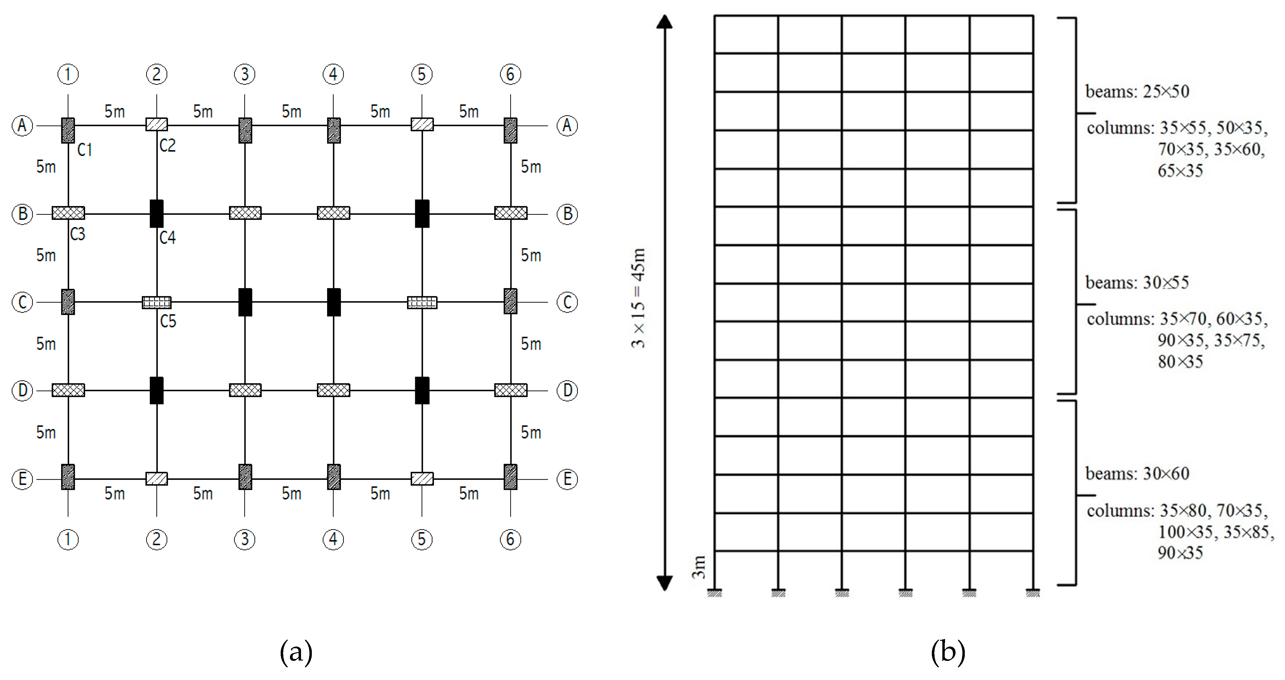
3. Properties of Structural Models

Five different RC frame building models, including 5-storey, 8-storey, 10-storey, 13-storey, and 15-storey are considered to represent mid-rise buildings. The buildings have been designed according to TBEC-2018 for DD-2 (10% probability to be exceeded in 50 years) seismic level. The importance factor (I) of the buildings and the soil class are taken as “1” and ZD, respectively.
The slab thicknesses including coatings were taken as 150 mm in all floors of all models to determine the dead load of the buildings. Live load was selected 2 kN / m2 [31]. Partition wall loads on the beams were taken into account as 3.25 kN / m. The axis spacing of the buildings in the x and y direction is 5 m, and the plan dimensions of the building are selected as 25 m and 20 m, respectively (Figure 1). Floor heights are considered as 3 m for all buildings.
Column sections of the 15-storey building are given in Figure 1a. During the design phase, 5 different rectangular sections were selected and the cross section of these columns was reduced at every 5 floors (Figure 1b). Beam and column sizes used in 15-, 13-, 10-, 8-, and 5-storey buildings are given in Table 2. The capacity design principles that meet ductility conditions were adopted during the design phase.
Concrete compressive strength and the yield strength of both longitudinal and transverse reinforcements are assumed to be 35 MPa and 420 MPa, respectively. Longitudinal reinforcement ratios of the column members range from 1.00–1.15%. Dominant vibration periods in x direction, seismic weight and lateral strength ratio (base shear/seismic weight) of the considered models are given in Table 3.
Three-dimensional (3D) models are created by using SAP2000, which is a general-purpose structural analysis program for dynamic analyses of structures [32]. Beam and column elements were modelled as nonlinear frame elements with lumped plasticity by defining plastic hinges at both ends of beams and columns. Damage level for each element is determined according to TBEC-2018. The nonlinear analysis is carried out using the effective stiffness of the cracked section properties per TBEC-2018; 0.35EIg for beams and 0.7EIg for columns (E: Concrete modulus of elasticity and Ig is moment of inertia for gross section). Several plastic hinge lengths have been proposed in the literature. For this study, half of the section depth is used for the plastic hinge length value as recommended in TBEC-2018.

4. Geotechnical Properties of Soil Profile

In this study, the seismic behaviors of the mid-rise RC frame buildings on soft soils are examined. Therefore, a soil profile with shear wave velocity of less than 600 m/s has been chosen [33,34]. According to TBEC-2018; the soil class ZD has a shear-wave velocity between 180 and 360 m/s. To meet these two criteria, the soil profile adopted from Ghandil’s work was used [25]. The soil profile consists of 3 different clay layers with a total height of 45 m. The geotechnical characteristics of the soil profile are given in Table 4. Vs, v, Cu, and ρ represent shear wave velocity, Poisson ratio, undrained cohesion, and soil density, respectively.
During the earthquake, the shear modulus and damping ratios of the soil change as shear strain increases. Seed and Iddris [35] proposed the equivalent linear method (ELM) for the shear modulus and damping curves corresponding to increasing strains. This method, in which iterative linear analysis is performed, uses the shear modulus (G/Gmax) and damping ratio (D) corresponding to the maximum strain on the soil.
Byrne [36] emphasized that the nonlinear effects cannot be directly captured in soil-structure interaction analysis since the equivalent linear method includes a linear approach. Byrne proposed to use the fully nonlinear method to directly reflect stress strain relations in a realistic way.
This study adapted the fully nonlinear model in order to characterize the real behavior of the soil in dynamic analysis. Damping and shear modulus relationships were taken into account depending on the shear strain values. Skeleton (backbone) curves were used to reflect hysteretic damping. The backbone curves suggested by Vucetic and Dobry [37] for clay layers are considered (Figure 2). Curve fitting has been carried out so that larger shear strains can better match the damping curves. A modified hyperbolic model is used in this paper and implemented in 1-D wave propagation software DEEPSOIL [38] to perform nonlinear site response analyses.

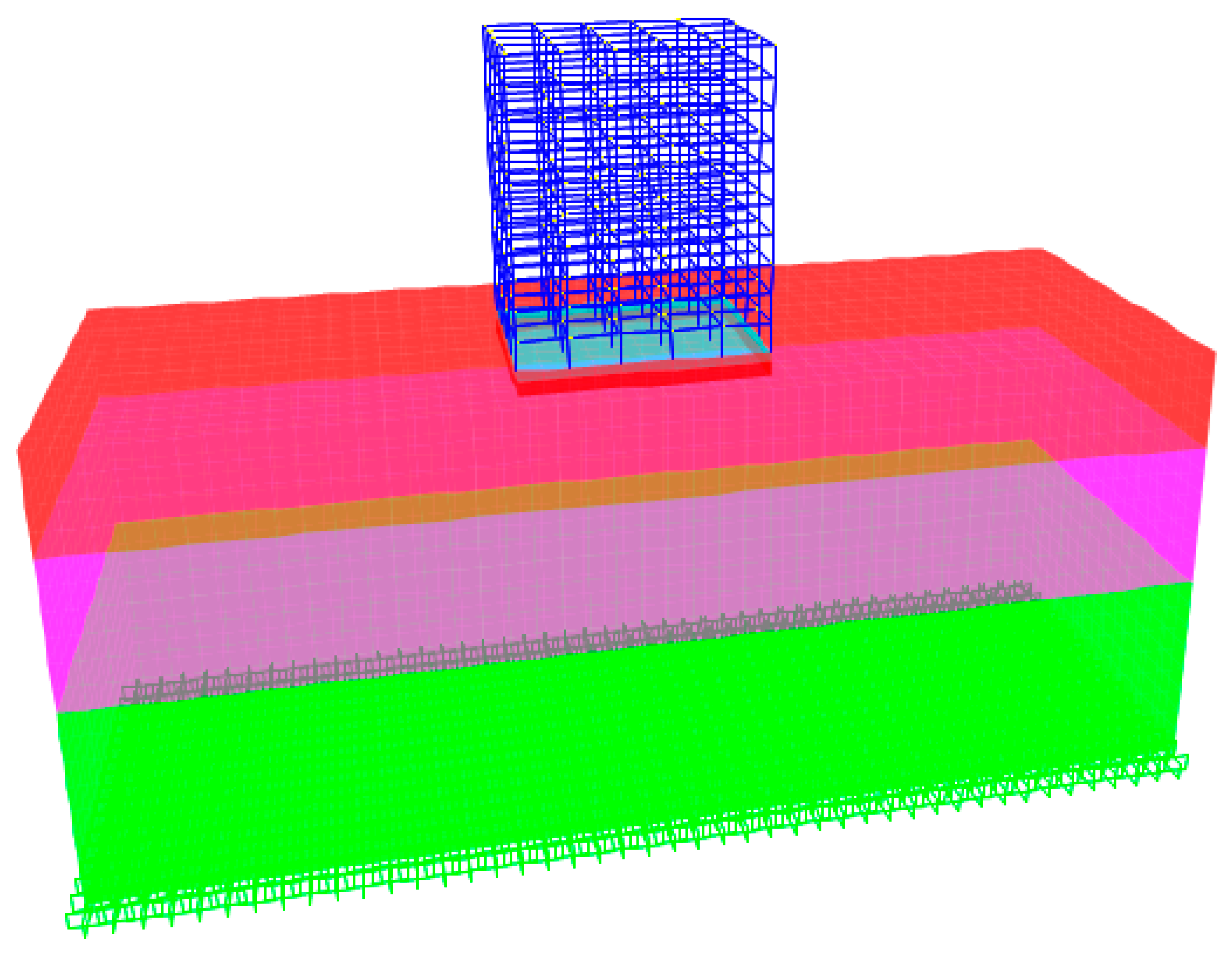
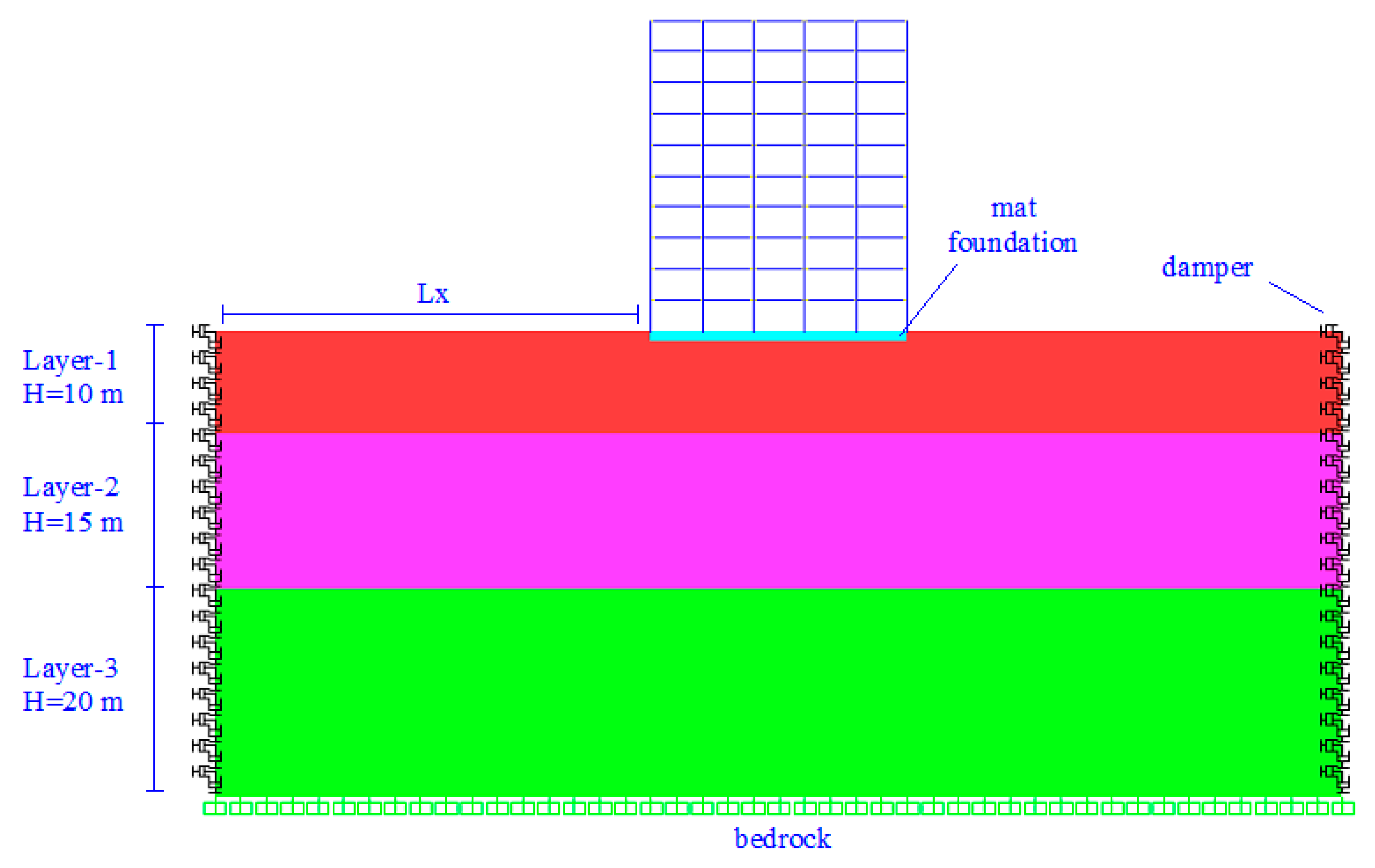
5. Description of the Soil-Structure Model

Inelastic soil-structure interaction models (SSI) were created in SAP2000. A 10-storey SSI model on three layers with depth of 45 m is given in Figure 3 as an example. In this model, the mat foundation is also reflected in the SSI system (Figure 4). The depth of the mat foundations is selected and designed as 0.5, 0.75, 1, 1.25, and 1.25 m for 5-, 8-, 10-, 13-, and 15-storey buildings, respectively. As the depth of foundations indicate, the mid-rise buildings have shallow foundation systems. The selected foundation depths are typical depths in practice. Assuming a perfect bond between the foundation and the surrounding soil, interface element is ignored. Thus, any possible relative displacement in the form of uplifting or sliding between the structure and the soil has been neglected [39].
Kocak and Mengi [40] emphasized that the rigid boundary condition is more appropriate and realistic boundary condition for simulation of the bedrock in dynamic soil-structure analysis. The boundary condition for the bedrock is assumed to be rigid in many studies [22,23,24,25] and [41,42,43]. In accordance with the mentioned previous studies, rigid boundary is defined for each node at the bottom surface of the soil medium in order to reflect the bedrock in this study. The soil profile consists of 3 different clay layers with a total height of 45 m. The thicknesses of these layers (from the ground surface) are 10, 15, and 20 m, respectively. Bedrock is located at a depth of 45 m. However, it should be noted that if the impedance contrast difference between the bedrock and the soil medium is high, it will not be appropriate to simulate the bedrock with the rigid boundary assumption [44].
The average shear wave velocity (Vs,avg) of the soil profile considered in this study is 228 m/s [25]. The fundamental frequency (f) of soil deposit is 1.19 Hz. According to Lachetl and Bard [45], the depth of bedrock can be determined approximately with d = Vs/4f. Based on this statement, the depth of bedrock in this study is expected to be around 48 m. As another study, according to the empirical formula proposed by Delgado et al. [46] (d = 55f−1.256) the bedrock depth could be 44 m. In order to be compatible with these related references, the bedrock depth was determined as 45 m.
Although the finite element modeling used for the soil profile has some limitations in geotechnical areas due to its physical dimensions, it is used effectively in many engineering applications. However, the full nonlinear 3D finite element analysis is still costly in terms of computational effort, load. Therefore, a reasonably limited model was created by using artificial or transmitting boundaries for finite element analysis of the dynamic soil-structure interaction problem as an alternative to very large soil profile modeling. This approach not only prevents unreal reflections against artificial boundaries presented in the mathematical model, but also avoids distorted results by taking into account radiation effects. Lysmer and Kuhlemeyer [47] proposed the application of viscous dampers that absorb reflected energy along the artificial boundary. In this study, the viscous boundary model, which was successfully employed by Livaoglu and Dogangun, is used [48,49]. In this model, dampers are placed along the normal and tangent of the boundary. Equivalent damping values are defined by ρV coefficients per unit area of the boundaries. Since the forces at the boundaries are equivalent to the forces generated in viscous dampers, the energy can be completely absorbed.
Ghosh and Wilson [50] stated that the effects of reflected waves can be neglected if the dampers are at a distance of 3–4 times plan dimensions and 2–3 times height of the foundation from the center of the structure. The building foundation dimensions used in the study are 25 × 20 m in x and y directions, respectively. According to reference above, the plan dimensions of the soil profile are selected as 110 × 40 m.

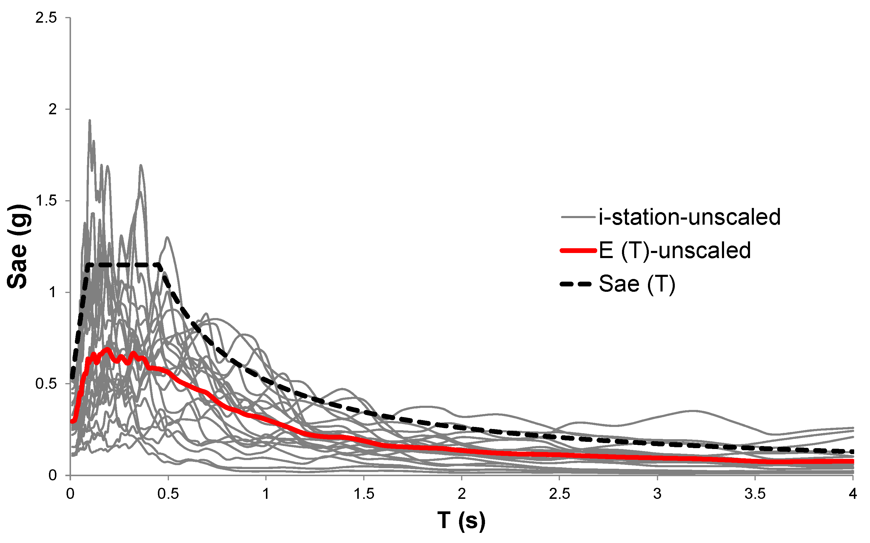
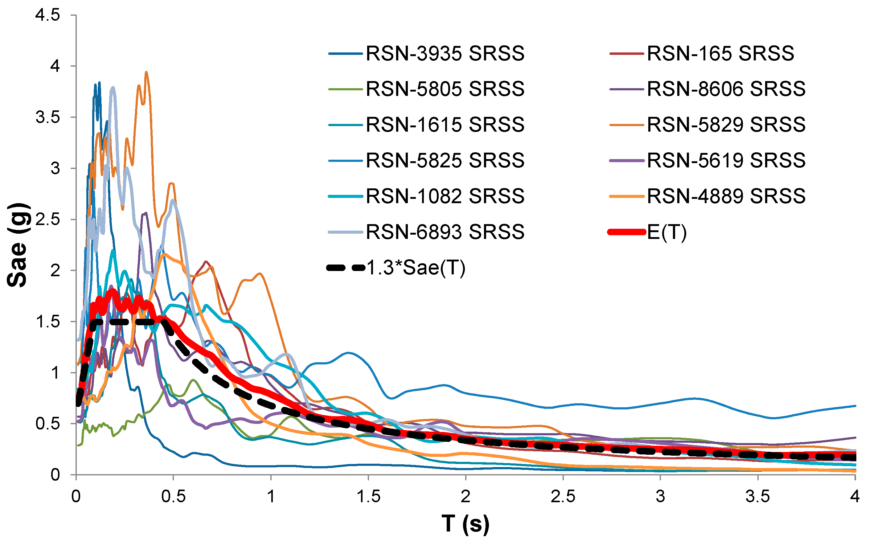
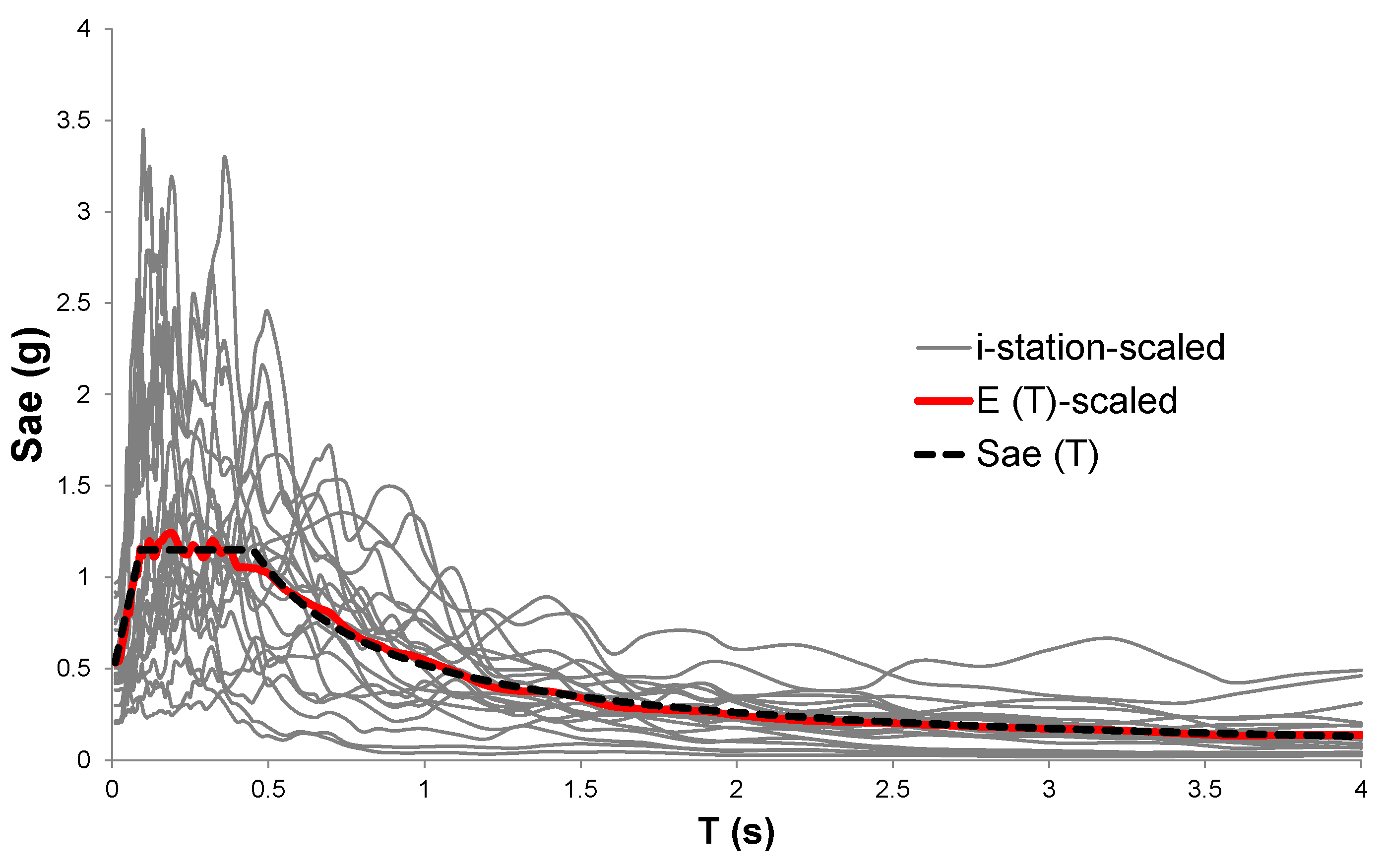
6. Selection and Scaling of Ground Motion Records

In nonlinear time history analyses, the use of real ground motion records is preferred due to their easily accessible databases. Due to variation in soil properties and station distances, the selection and scaling of ground motion records is significantly important to reflect earthquake hazards properly.
Optimization techniques are frequently used for selecting and scaling earthquake records that comply with the earthquake code [51]. A solution such as a constrained optimization problem can be implemented by targeting the response spectra in the earthquake design code. In this study, acceleration records that provide design acceleration spectrum conditions of TBEC-2018 have been selected and scaled. According to TBEC-2018, a minimum of 11 pairs of ground motion records are required for the 3D time history analysis. In addition, the number of record and record pairs to be selected from the same earthquake event should not exceed three. A square root of the sum of the squares (SRSS) spectrum needs to be constructed by using the scaled horizontal components of each ground motion where the same scale factor is applied for both components. The mean of the SRSS spectra for the scaled ground motions should be more than 1.3 times the target code values between the 0.2Tp and 1.5Tp period range, where Tp is the natural period of the building model.
The PEER (Pacific Earthquake Engineering Research) database has been used for the selection earthquake records used in the current study [52]. The criteria for selection of acceleration records were given in Table 5. The earthquake magnitudes, Mw, were assumed to be between 4.5 and 7.5 while the station distances were limited to be between 5 and 50 km. Records with peak ground acceleration (PGA) value of 0.1g and above were preferred. In order to represent the soil class ZD, the shear wave velocity Vs was chosen to be between 180 and 360 m/s.
In this study, the seismic level (DD-2) with 10% probability of exceedance in 50 years in TBEC-2018 is taken as target spectrum. The parameters controlling the shape of the design spectrum in order to draw horizontal design spectrum are also given in Table 5. These parameters; SDS, SD1, TA, TB, respectively, represent the short-period design spectral acceleration coefficient, the design spectral acceleration coefficient corresponding to a one-second period, and the corner periods of the horizontal elastic spectrum.
The earthquake set with 11 record pairs compatible with the selected target spectrum was obtained using the Differential Evolution Algorithm [53]. The unscaled spectrum and averages of the selected records are given in Figure 5.
The SRSS spectrums belonging to the 11 acceleration record pairs and their average spectrum, E(T), are given in Figure 6. In addition, the 1.3 times target spectrum Sae(T) for the soil class ZD is given in the same figure. The acceleration spectrum and average spectrum of 11 scaled acceleration record pairs are plotted in Figure 7. The properties of the selected earthquake records and scale factors are provided in Table 6. The scale factors ranging between 1.48 and 1.95 are reasonably well.
The selected acceleration records were obtained from the ground surface. While these records are used directly for the fixed-base (FB) models, they cannot be used directly for the SSI models. In the SSI models, earthquake records are implemented from the bedrock. For this reason, the DEEPSOIL program was used to convert the surface (input) records to the corresponding records (output) at the bedrock. This process is called “deconvolution”. The surface motions were applied from the top of one-dimensional (1D) free-field soil column, and bedrock motions were calculated. A sample record is given in Figure 8. During the deconvolution process; resonance has occurred for one of the horizontal directions of RSN1615 acceleration record (RSN1615-H1), and it is removed from the acceleration record set. Therefore, 21 acceleration records were used in this study.

7. Correlation Analyses for Ground Motions Parameters

Nonlinear time history analyses were performed using 21 different acceleration records for 5 different building models with SSI. As a result of the analyses, the roof displacement demands of the buildings were obtained. These displacement demands were normalized with the building height, and roof drift ratios (RDR) were calculated. Table 7 lists roof drift ratios 15-, 13-, 10-, 8-, and 5-story buildings, separately. Besides, the average RDR value of 5 different building models is given for the scaled 21 ground motion records.
The variation in RDR values within ground motion records of each building is obvious. Similar variation exists within RDR values of different buildings subjected to the same record. Although there are several extreme values for 5- or 15-story buildings, the average RDR value of 15-, 13-, 10-, 8-, and 5-storey buildings is a valuable indicator to represent damage of a ground motion record. In this way, it is aimed to reduce the effect of building height in the evaluation of buildings with different heights [20,21].
Correlations between RDR of each building model and ground motion parameters (GMP) are given in Table 8. In addition, correlation values were given for each record by calculating the mean of the RDRs of all building models. The values of the GMPs were determined using the software SeismoSignal for the acceleration records corresponding to the ground surface of the soil profile.
The parameters in Table 8 are given in 4 groups as velocity, frequency, displacement, and acceleration. These parameters in each group were ranked from the highest R2 to the lowest. Table 8 obviously shows that the parameters in velocity groups are very effective in estimating the damage potential of building models. On the other hand, the correlation values of the parameters in the displacement and acceleration groups are too low.
Figure 9 plots roof drift ratio (RDR) of building models versus velocity related parameter values. As it is seen, there are five RDR values for each ground motion parameter value. The equation for their correlation and R2 values are also given on the figure. It is obvious that RDR values of five building models vary within a narrow range. Therefore, average RDR values of five buildings are also used to look for a possible better correlation. The R2 values calculated using the average RDR values are listed in the last column of Table 8 and plotted in Figure 10. All velocity related parameters except CAV have R2 values greater than 0.70. The lowest correlation value was obtained for the A95 parameter.
Figure 11 plots average RDR of all building models versus velocity related parameter values as well as the equation for their correlation and R2 values. When all models with a single RDR values for each ground motion record are examined, HI is the strongest correlation in the velocity group and its R2 value was calculated as 0.914. In addition, Vrms, VSI, SED, SMV, and PGV parameters in the velocity group also provide a strong relationship for the roof drift ratio (RDR) estimates. If the building models are examined separately, HI is the best parameter with R2 value of 0.923 for 5-storey buildings.
The estimated RDR values calculated using the equations given in Figure 11 are normalized with the analysis results listed in the last column of Table 7. The average, standard deviation, and coefficient of variation (CoV) values are given in Table 9 for the velocity related parameters. The lowest coefficient of variation value, which shows the effect of scattering on the mean, is obtained for the HI parameter. The highest CoV value among these six parameters is observed for SMV.

8. Optimization Study for Better Correlation

In the previous section, the correlation between ground motion parameters and their damage potentials using roof drift ratios was investigated for each single parameter. HI parameter is found out as the best single parameter to represent damage potential of ground motion record. This section investigates whether the combination of multiple parameters can reflect the damage potential better than a single ground motion parameter. The aim is to seek a higher damage correlation using several ground motion parameters among twenty of them. Determining these several parameters and their weight coefficients is a complex problem. The process of selecting parameters and determining the weight coefficients has been considered as an optimization problem. A new equation that gives a better correlation was investigated by minimizing the sum of squares of errors between the displacement demands obtained from the combined parameters and the analysis results. Differential Evolution (DE) algorithm was used for the optimization purposes. Since the aim is to represent the damage correlation using the minimum number of parameters, the number of parameters was selected between two and six for the combined multiple parameter approach.
The DE algorithm requires a mathematical expression to estimate the roof drift ratio (RDR) with ground motion parameters. For this reason, five equations containing 2, 3, 4, 5, and 6 ground motion parameters and their weight coefficients are used. Linear equations were preferred due to their simple form and easiness to use. The terms (xi) given in Equations (1) to (5) refer to the weight coefficients of the parameters. These variables can take negative or positive values. Pi represents randomly selected parameters among the twenty parameters. Although parameters are not represented in variable terms (xi), variables consisting of integers are defined for the selection of these parameters.
E 1   = x 1 + x 2 P 1 + x 3 P 2
E 2   = x 1 + x 2 P 1 + x 3 P 2 + x 4 P 3
E 3   = x 1 + x 2 P 1 + x 3 P 2 + x 4 P 3 + x 5 P 4
E 4   = x 1 + x 2 P 1 + x 3 P 2 + x 4 P 3 + x 5 P 4 + x 6 P 5
E 5   = x 1 + x 2 P 1 + x 3 P 2 + x 4 P 3 + x 5 P 4 + x 6 P 5 + x 7 P 6
After determining the decision variables and equation form, the objective function should be defined. If the errors between the analysis results and the RDR values obtained from the equations (Ei) are minimal, there is a stronger relationship between RDR and the combined multiple parameter approach. Therefore, the objective function defined in Equation (6) reflects the minimization of mean square errors (MSE), where ei represents the error between the predicted value and the analysis result for each parameter, and n is the number of records.
min f x   = 1 n e i 2 n + h 1 x +   h 2 x
The h1(x) and h2(x) in Equation (6) represent the penalty functions given in Equations (7) and (8). These functions provide constraints to be taken into account. The penalty function helps to minimize the objective function effectively on constraints. When the constraints provide the necessary conditions, the penalty function becomes zero, otherwise, the penalty function becomes active [54]. Two penalty coefficients (PCi) were applied for each constraint separately.
h 1 x   =   PC 1 if   the   same   parameter   is   used   more   than   once 0 otherwise
h 2 x   =   0 if   E 1 ,   E 2 > 0 PC 2 otherwise
The sensitivity of the population size (NP), mutation ratio (CR), and scaling factor (F) parameters on the results in the DE algorithm was examined. A total of 63 groups (3 × 7 × 3 = 63) were formed for 3 different population sizes, 7 different crossover ratios, and 3 different scaling factors. Ten analyses were carried out for each group. A total of 3150 analyses were performed for five equation forms. The maximum number of iterations for all analyses was chosen as 1000.
The E1–E5 Equations obtained from the optimization analyses are given in Equations (9)–(13). The HI and SED represent the RDR for the two-parameter approach, while the three-parameter approach uses HI, SED, and Ia parameters. The Tm is an additional parameter for the four-parameter approach. Although it is not forced, the existence of similar parameters shows their strong correlation with RDR values for the first three combined multiple parameter approach equations. The other two equations include more parameters. However, HI appears in all equations. The R2 value was calculated as 0.94, 0.94, 0.95, 0.93, and 0.90 for E1, E2, E3, E4, and E5, respectively. The best R2 value is calculated for E3 as 0.95. If the HI and SED parameters in velocity group are used alone, their R2 values are 0.91 and 0.82, respectively. The R2 values are 0.52 and 0.27 for Tm and Ia parameters. Their combined use increases R2 value to 0.95. The units in E1−E5 are ground acceleration (g), second (s), and meter (m) as given in Table 1.
E 1   = 0.034 + 0.1751   SED + 0.298   HI
E 2   = 0.0275 0.0175   I a + 0.1853   SED + 0.3495   HI
E 3   = 0.096 + 0.1922   SED + 0.3991   HI 0.0269   I a 0.193   T m
E 4   = 0.306 + 0.1946   SED + 1.118   HI 0.329   T m 0.695   VSI 0.00957   CAV
E 5   = 0.248 2.8   V max A max + 1.56   V rms 1.414   ASI + 0.183   VSI + 1.506   SMV + 0.16   HI
The roof drift ratio (RDR) values estimated using the proposed E1−E5 given in Equations (9)–(13) were compared with analyses results. Statistics for the estimated to analyses result values (RDRest/RDRanly) are summarized in Table 10. The single parameter estimates for velocity related parameters are also provided in the table. Although the mean values have a narrow band, the differences between maximum and minimum values of the RDRest/RDRanly ratio are remarkable for the single parameter use. While the E2 gives the best mean value, the SMV gives the worst. However, the E3 has less scatter than other parameters and equations. Coefficient of Variation (CoV) values of the other parameters and equations are normalized with E3 in the last column of Table 10. E1 and E4 are the closest equations to the E3 with a difference of 6%. Moreover, it is seen that HI has significantly lesser deviation compared to the other single parameters. It should be kept in mind that E3 requires 4 parameters. Therefore, the use of E1 with 2 parameters is a reasonable choice in estimating roof drift of RC frame buildings having 5 to 15 floors.
RDR values obtained for common parameters (HI, PGV, and VSI) and E1−E5 are plotted in Figure 12. The different estimated to analysis roof drift ratios are also drawn on the figure as lines a, b, and c (RDRestimated/RDRanalysis = 1.3, 1 and 0.7) to show the scatter more clearly. Figure 12 shows that all estimated values of the E1–E5 are within a and c lines, while the other parameters, especially the PGV, have a considerable number of estimates out of these lines.

9. Summary and Conclusions

Damage potentials of reinforced concrete buildings are defined with ground motion parameters in the literature. Fixed base models were preferred in the present studies, and soil-structure-interaction (SSI) has been neglected. However, rotations of foundation and rocking motions in soft soils have a significant effect on the lateral displacement demands of mid-rise or taller buildings. These phenomenon are ignored by using the fixed base model. This study investigates the correlation of ground motion parameters (GMP) with inelastic displacement demands of mid-rise RC frame buildings with no shear walls considering soil structure interaction. In order to reflect the nonlinear behavior of soil, a fully nonlinear method has been considered. The 5-, 8-, 10-, 13-, and 15-storey reinforced concrete buildings without any structural irregularity are modelled using SSI to represent mid-rise buildings 21 acceleration records compatible with TBEC-2018 were selected and scaled. The 20 GMP of each selected record were obtained. The roof drift ratio (RDR) is used for demand measure and it is obtained as inelastic displacement demands normalized by the building height. Total of 105 3D nonlinear time history analyses were carried out, and the roof displacement demands were obtained from these analyses. The findings obtained are summarized below:
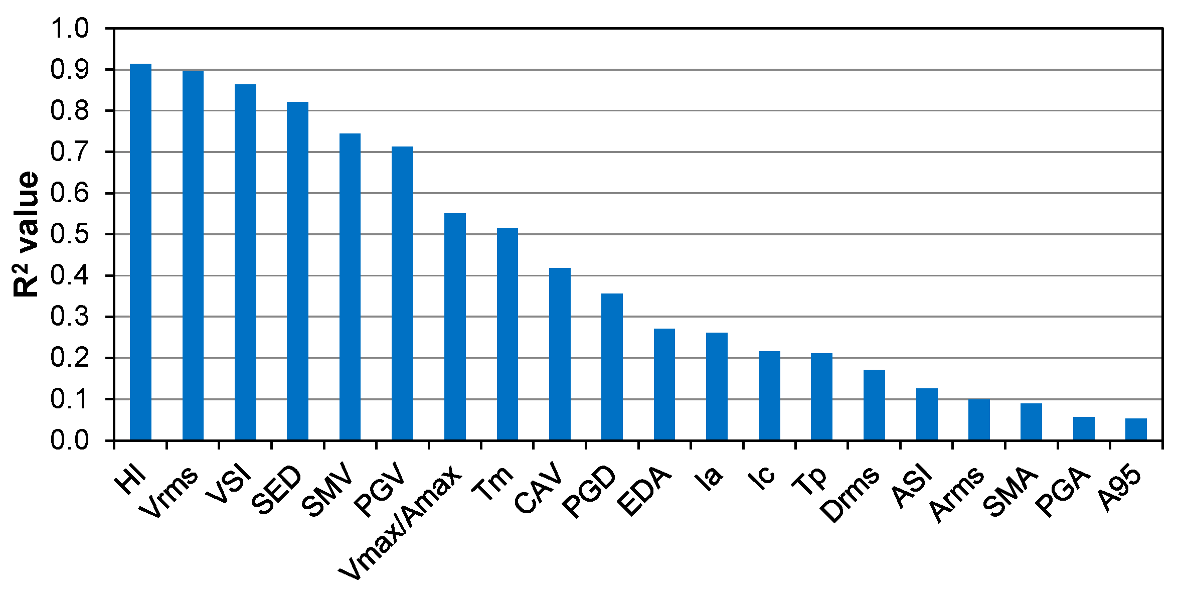
  • The velocity related parameters are very effective in estimating the damage potential of building models. On the other hand, the correlation values of the parameters in the displacement and acceleration groups are too low.
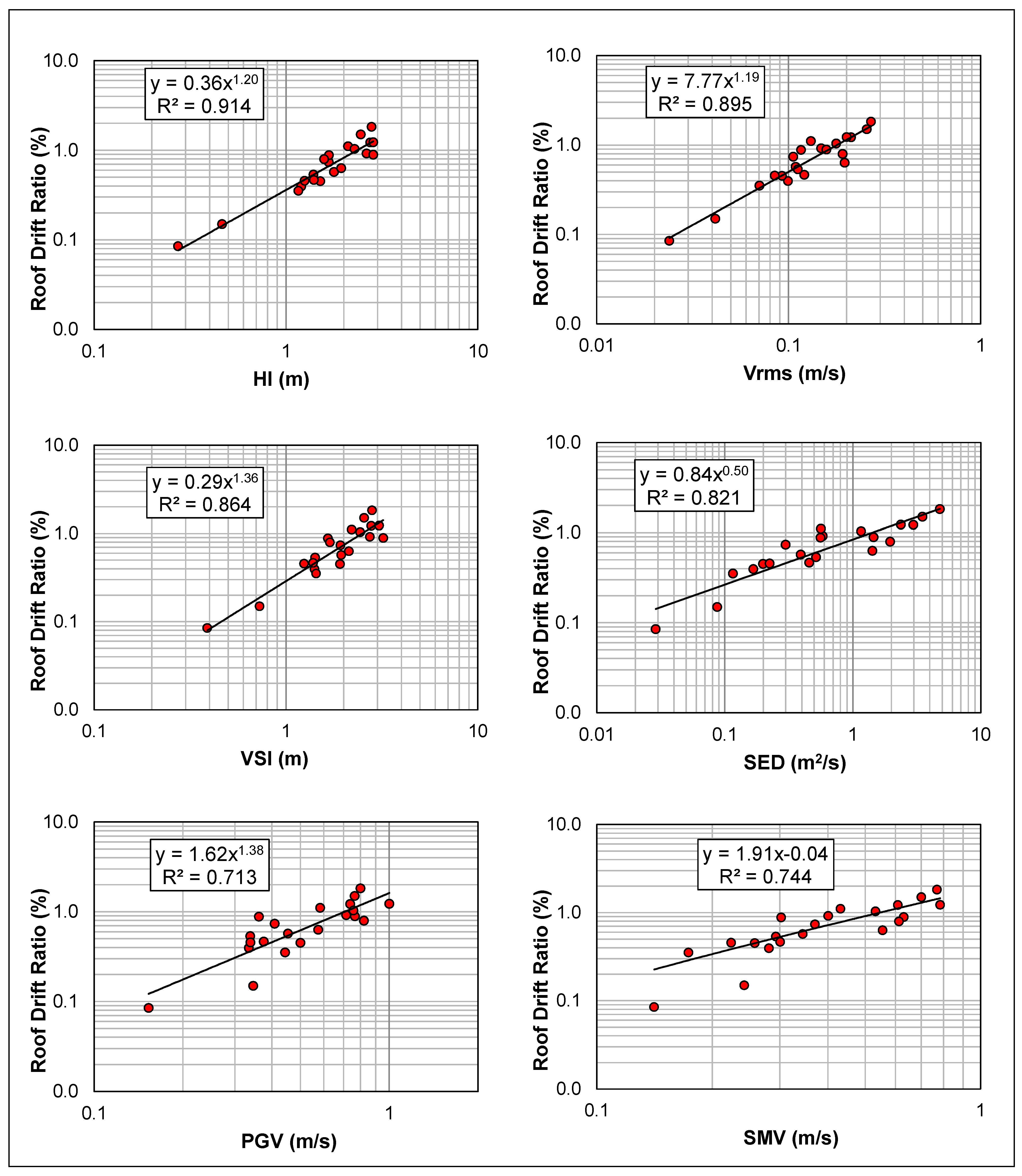
  • Housner Intensity (HI) has the strongest correlation in the all parameters with its R2 value of 0.914. Moreover, Vrms, VSI, SED, SMV, and PGV have R2 values greater than 0.70. The lowest correlation value was obtained for the A95 parameter.
  • Being one of the common parameters, PGA has a low correlation factor as observed in many other studies such as Cao and Ranogh [17], Yakut and Yılmaz [19], and Ozmen and Inel [20].
  • HI shows the lowest scatter on the mean values of roof drift ratios by having the lowest value of the coefficient of variation (CoV).
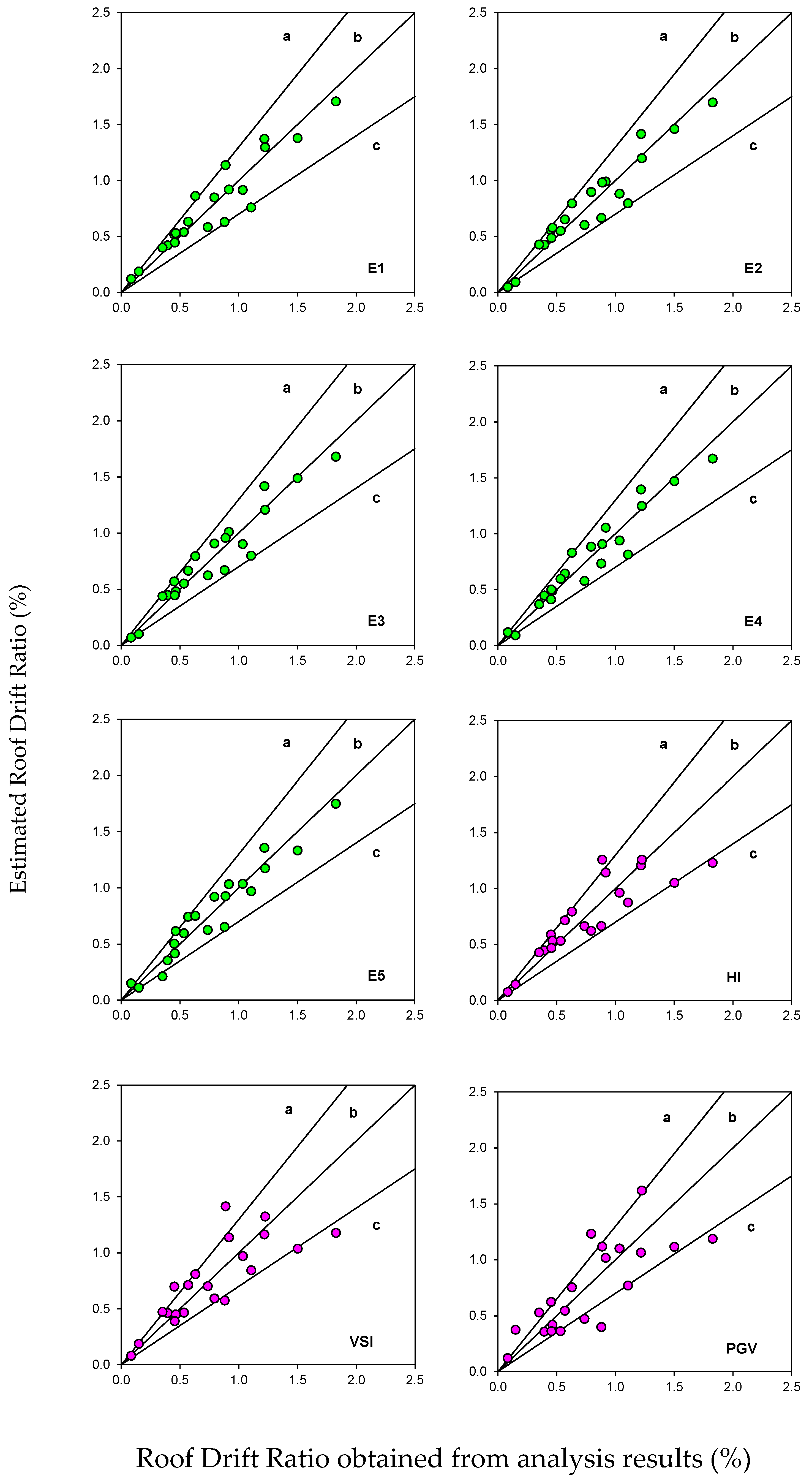
  • This paper seeks a new combined multiple ground motion parameter from their combinations using DE algorithm in order to reflect the damage potential better than a single ground motion parameter. Five different equations were proposed as combined multiple ground motion parameters having R2 values between 0.95 and 0.93 for mid-rise RC frame buildings on soft soil deposit.
  • The best roof drift ratio estimates are obtained using equation E3, which is a combination of Ia, SED, Tm, and HI parameters. On the other hand, the use of E1 equation including SED and HI parameters provides reasonably well estimates.
  • The use of combined multiple parameters can be effective in determining seismic damages by improving the scatter at least 24% compared to the use of a single parameter.
This study shows that commonly used parameters such as HI, Vrms, VSI, and PGV reflect inelastic displacement demands of mid-rise buildings as a damage indicator on soft soil deposit reasonably well. The optimization algorithm improves the displacement demand estimates by using multiple combined parameters. The outcomes obviously show that the best roof drift ratio estimates are obtained when an equation as a combination of Ia, SED, Tm, and HI parameters is used. On the other hand, the use of an equation including SED and HI parameters provides reasonably good estimates. The use of a single-parameter (HI), two-parameter equation (HI and SED), or four parameter-equation is related to the simplicity and accuracy. It is clear that a single-parameter equation can provide reasonably acceptable results with a certain scatter while the scatter decreased as the number of parameters increases. The use of equations provided in this paper can play an important role in determining or assessing of seismic damage to buildings on soft soils. It should be noted that the investigated buildings in this study are mid-rise RC frame buildings with no structural irregularity. Therefore, the results and produced equations are valid for those building types and may not give accurate results for the buildings with shear walls or with structural irregularity.

Author Contributions

Conceptualization, methodology, validation, investigation, data curation, M.K. and M.I.; resources, software, writing—original draft preparation, visualization M.K.; writing—review and editing, supervision M.I. All authors have read and agreed to the published version of the manuscript.

Funding

This research received no external funding.

Institutional Review Board Statement

Not applicable.

Informed Consent Statement

Not applicable.

Data Availability Statement

The data presented in this study are available on request from the corresponding author.

Conflicts of Interest

The authors declare no conflict of interest.

References

  1. Akkar, S.; Ozen, O. Effect of peak ground velocity on deformation demands for SDOF systems. Earthq. Eng. Struct. Dyn. 2005, 34, 1551–1571. [Google Scholar] [CrossRef]
  2. Cabanas, L.; Benito, B.; Herraiz, M. An approach to the measurement of the potential structural damage of earthquake ground motions. Earthq. Eng. Struct. Dyn. 1997, 26, 79–92. [Google Scholar] [CrossRef]
  3. Elenas, A. Interdependency between seismic acceleration parameters and the behavior of structures. Soil Dyn. Earthq. Eng. 1997, 16, 317–322. [Google Scholar]
  4. Elenas, A. Correlation between seismic acceleration parameters and overall structural damage indices of buildings. Soil Dyn. Earthq. Eng. 2000, 20, 93–100. [Google Scholar] [CrossRef]
  5. Wu, Y.-M.; Hsiao, N.-C.; Teng, T.-L. Relationships between Strong Ground Motion Peak Values and Seismic Loss during the 1999 Chi-Chi, Taiwan Earthquake. Nat. Hazards 2004, 32, 357–373. [Google Scholar] [CrossRef] [Green Version]
  6. Kramer, S.L.; Mitchell, R.A. Ground Motion Intensity Measures for Liquefaction Hazard Evaluation. Earthq. Spectra 2006, 22, 413–438. [Google Scholar] [CrossRef]
  7. Riddell, R. On Ground Motion Intensity Indices. Earthq. Spectra 2007, 23, 147–173. [Google Scholar] [CrossRef]
  8. Kadas, K.; Yakut, A.; Kazaz, I. Spectral Ground Motion Intensity Based on Capacity and Period Elongation. J. Struct. Eng. 2011, 137, 401–409. [Google Scholar] [CrossRef]
  9. Cao, V.V.; Ronagh, H.R. Correlation between parameters of pulse-type motions and damage of low-rise RC frames. Earthq. Struct. 2014, 7, 365–384. [Google Scholar] [CrossRef]
  10. Takizawa, H.; Jennings, P.C. Collapse of a model for ductile reinforced concrete frames under extreme earthquake motions. Earthq. Eng. Struct. Dyn. 1980, 8, 117–144. [Google Scholar] [CrossRef]
  11. Nau, J.M.; Hall, W.J. Scaling Methods for Earthquake Response Spectra. J. Struct. Eng. 1984, 110, 1533–1548. [Google Scholar] [CrossRef]
  12. Kostinakis, K.; Fontara, I.K.; Athanatopoulou, A.M. Scalar Structure-Specific Ground Motion Intensity Measures for Assessing the Seismic Performance of Structures: A Review. J. Earthq. Eng. 2018, 22, 630–665. [Google Scholar] [CrossRef]
  13. Elnashai, A.; Sarno, L.D. Fundamentals of Earthquake Engineering; John Wiley & Sons Ltd.: West Sussex, UK, 2008. [Google Scholar]
  14. Moustafa, A.; Takewaki, I. Characterization of earthquake ground motion of multiple sequences. Earthq. Struct. 2012, 3, 629–647. [Google Scholar] [CrossRef]
  15. Elenas, A.; Meskouris, K. Correlation study between seismic acceleration parameters and damage indices of structures. Eng. Struct. 2001, 23, 698–704. [Google Scholar] [CrossRef]
  16. Nanos, N.; Elenas, A.; Ponterosso, P. Correlation of different strong motion duration parameters and damage indicators of reinforced concrete structures. In Proceedings of the 14th World Conference on Earthquake Engineering, Bejing, China, 12–17 October 2008. [Google Scholar]
  17. Cao, V.V.; Ronagh, H.R. Correlation between seismic parameters of far-fault motions and damage indices of low-rise reinforced concrete frames. Soil Dyn. Earthq. Eng. 2014, 66, 102–112. [Google Scholar]
  18. Kostinakis, K.G.; Athanatopoulou, A.M. Evaluation of scalar structure-specific ground motion intensity measures for seismic response prediction of earthquake resistant 3D buildings. Earthq. Struct. 2015, 9, 1091–1114. [Google Scholar] [CrossRef]
  19. Yakut, A.; Yılmaz, H. Correlation of Deformation Demands with Ground Motion Intensity. J. Struct. Eng. 2008, 134, 1818–1828. [Google Scholar] [CrossRef]
  20. Ozmen, H.B.; Inel, M. Damage potential of earthquake records for RC building stock. Earthq. Struct. 2016, 10, 1315–1330. [Google Scholar] [CrossRef]
  21. Ozmen, H.B. Developing hybrid parameters for measuring damage potential of earthquake records: Case for RC building stock. Bull. Earthq. Eng. 2016, 15, 3083–3101. [Google Scholar] [CrossRef]
  22. Tabatabaiefar, H.R.; Massumi, A. A simplified method to determine seismic responses of reinforced concrete moment resisting building frames under influence of soil–structure interaction. Soil Dyn. Earthq. Eng. 2010, 30, 1259–1267. [Google Scholar] [CrossRef]
  23. Fatahi, B.; Tabatabaiefar, H.R. Fully nonlinear versus equivalent linear computation method for seismic analysis of midrise buildings on soft soils. Int. J. Geomech. ASCE 2014, 14, 04014016. [Google Scholar] [CrossRef]
  24. Ghandil, M.; Behnamfar, F. The near-field method for dynamic analysis of structures on soft soils including inelastic soil–structure interaction. Soil Dyn. Earthq. Eng. 2015, 75, 1–17. [Google Scholar] [CrossRef]
  25. Ghandil, M.; Behnamfar, F. Ductility demands of MRF structures on soft soils considering soil-structure interaction. Soil Dyn. Earthq. Eng. 2017, 92, 203–214. [Google Scholar] [CrossRef]
  26. Borja, R.I.; Wu, W.; Amies, A.P.; Smith, H.A. Nonlinear Lateral, Rocking, and Torsional Vibration of Rigid Foundations. J. Geotech. Eng. 1994, 120, 491–513. [Google Scholar] [CrossRef]
  27. Carbonari, S.; Dezi, F.; Leoni, G. Linear soil-structure interaction of coupled wall-frame structures on pile foundations. Soil Dyn. Earthq. Eng. 2011, 31, 1296–1309. [Google Scholar] [CrossRef]
  28. TBEC-2018, (Turkish Building Earthquake Code). Specifications for Buildings to Be Built in Seismic Areas; Ministry of Public Works and Settlement: Ankara, Turkey, 2018.
  29. Kramer, S.L. Geotechnical Earthquake Engineering; Prentice-Hall: Englewood Cliffs, NJ, USA, 1996. [Google Scholar]
  30. Seismosoft. SeismoStruct 2016 Release-1—A Computer Program for Static and Dynamic Nonlinear Analysis of Framed Structures. Available online: http://www.seismosoft.com (accessed on 29 July 2017).
  31. The Calculation Values of Loads Used in Designing Structural Element; Turkish Standard, (TS498); Turkish Standard Institute: Ankara, Turkey, 1997.
  32. Finite Element Analysis and Design of Structures; Sap2000 CSI, Computers and Structures Inc: Berkeley, CA, USA, 1995.
  33. Velestos, A.S.; Prasad, A.M. Seismic interaction of structures and soils: Stochastic approach. J. Struct. Eng. ASCE 1989, 115, 935–956. [Google Scholar]
  34. Tabatabaiefar, S.H.R.; Fatahi, B.; Samali, B. Seismic Behavior of Building Frames Considering Dynamic Soil-Structure Interaction. Int. J. Géoméch. 2013, 13, 409–420. [Google Scholar] [CrossRef]
  35. Seed, H.B.; Idriss, I.M. Influence of Soil Conditions on Ground Motions During Earthquakes. J. Soil Mech. Found. Div. 1969, 95, 99–137. [Google Scholar] [CrossRef]
  36. Byrne, P.M.; Naesgaard, E.; Seid-Karbasi, M. Analysis and design of earth structures to resist seismic soil liquefaction. In Proceedings of the 59th Canadian Geotechnical Conf. and 7th Joint CGS/IAH-CNC Ground-Water Specialty Conf., Canadian Geotechnical Seciety, Richmond BC, Canada, 1–4 October 2006. [Google Scholar]
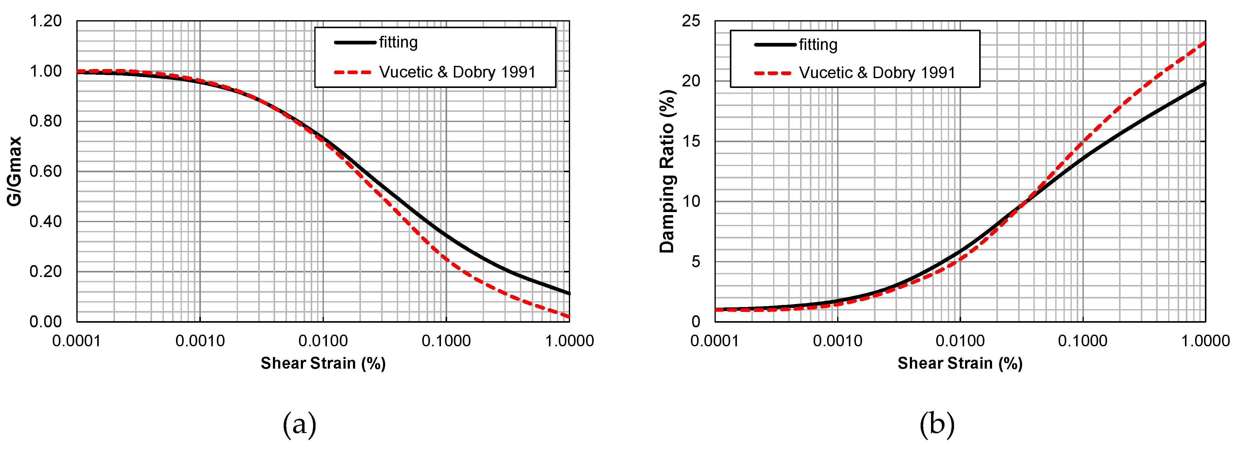
  37. Vucetic, M.; Dobry, R. Effect of Soil Plasticity on Cyclic Response. J. Geotech. Eng. 1991, 117, 89–107. [Google Scholar] [CrossRef]
  38. Hashash, Y.M.A.; Musgrove, M.I.; Harmon, J.A.; Ilhan, O.; Xing, G.; Numanoglu, O.; Groholski, D.R.; Phillips, C.A.; Park, D. DEEPSOIL, Version 7.0; Board of Trustees of Univ. of İllinois at Urbana-Champaign: Urbana, IL, USA, 2020. [Google Scholar]
  39. Scarfone, R.; Morigi, M.; Conti, R. Assessment of dynamic soil-structure interaction effects for tall buildings: A 3D numerical approach. Soil Dyn. Earthq. Eng. 2020, 128, 105864. [Google Scholar] [CrossRef]
  40. Kocak, S.; Mengi, Y. A Simple Soil-structure Interaction Model. Appl. Math. Model. 2000, 24, 607–635. [Google Scholar] [CrossRef]
  41. Dutta, C.H.; Roy, R. A Critical Review on Idealization and Modelling for Interaction among Soil–Foundation–Structure System. Comput. Struct. 2002, 80, 1579–1594. [Google Scholar] [CrossRef]
  42. Spyrakos, C.; Maniatakis, C.; Koutromanos, I. Soil–structure interaction effects on base-isolated buildings founded on soil stratum. Eng. Struct. 2009, 31, 729–737. [Google Scholar] [CrossRef]
  43. Zheng, J.; Takeda, T. Effects of soil-structure interaction on seismic response of PC cable-stayed bridge. Soil Dyn. Earthq. Eng. 1995, 14, 427–437. [Google Scholar] [CrossRef]
  44. Pitilakis, K.; Terzi, V. Experimental and Theoretical SFSI Studies in a Model Structure in Euroseistest. In Special Topics in Earthquake Geotechnical Engineering; Sakr, M., Ansal, A., Eds.; Springer: Dordrecht, The Netherlands, 2012; Volume 16, pp. 175–215. [Google Scholar] [CrossRef]
  45. Lachetl, C.; Bard, P.-Y. Numerical and Theoretical Investigations on the Possibilities and Limitations of Nakamura’s Technique. J. Phys. Earth 1994, 42, 377–397. [Google Scholar] [CrossRef]
  46. Delgado, J.; Lopez Casado, C.; Estevez, A.; Giner, J.; Cuenca, A.; Molina, S. Mapping soft soils in the Segura river walley (SE Spain): A case study of microtremors as an exploration tool. J. Appl. Geophys. 2000, 45, 19–32. [Google Scholar] [CrossRef]
  47. Kuhlemeyer, R.L.; Lysmer, J. Finite element method accuracy for wave propagation problems. J. Soil Mech. Found. Div. ASCE 1973, 99, 421–427. [Google Scholar] [CrossRef]
  48. Livaoglu, R.; Dogangun, A. Effect of foundation embedment on seismic behavior of elevated tanks considering fluid–structure-soil interaction. Soil Dyn. Earthq. Eng. 2007, 27, 855–863. [Google Scholar] [CrossRef]
  49. Livaoglu, R.; Cakir, T.; Dogangun, A.; Aytekin, M. Effects of back fill on seismic behavior of rectangular tanks. Ocean Eng. 2011, 38, 1161–1173. [Google Scholar] [CrossRef]
  50. Ghosh, S.; Wilson, E.L. Dynamic Stress Analysis of Axi-Symmetric Structures under Arbitrary Loading; University of California: Berkeley, CA, USA, 1969. [Google Scholar]
  51. Fahjan, Y.M. Selection and scaling of real earthquake accelerograms to fit the Turkish Design Spectra. Teknik Dergi 2008, 19, 4423–4444. [Google Scholar]
  52. PEER Ground Motion Database. Available online: https://ngawest2.berkeley.edu/ (accessed on 19 March 2011).
  53. Storn, R.; Price, K. Differential evolution a simple and efficient adaptive scheme for global optimization over continuous spaces. J. Glob. Optim. 1997, 11, 341–359. [Google Scholar] [CrossRef]
  54. Kamal, M.; Inel, M. Optimum design of reinforced concrete continuous foundation using differential evolution algorithm. Arab. J. Sci. Eng. 2019, 44, 8401–8415. [Google Scholar] [CrossRef]
Figure 1. (a) Plan views of first floor of 15-storey building, (b) elevation view.
Buildings 11 00125 g001
Figure 2. (a) Relationship between G/Gmax and shear strain, (b) relationship between material damping ratio and shear strain.
Buildings 11 00125 g002
Figure 3. 3D view of 10s- soil-structure-interaction (SSI) model.
Buildings 11 00125 g003
Figure 4. A section along the x direction of 10-storey SSI model.
Buildings 11 00125 g004
Figure 5. The spectrum of unscaled acceleration records.
Buildings 11 00125 g005
Figure 6. The square root of the sum of the squares (SRSS) spectrum of scaled acceleration records.
Buildings 11 00125 g006
Figure 7. The spectrum of scaled acceleration records.
Buildings 11 00125 g007
Figure 8. Comparison of the motion of the RSN1082-H2 record of Northridge earthquake on the surface and bedrock (a) acceleration record; (b) acceleration spectra.
Buildings 11 00125 g008
Figure 9. The correlation for roof drift ratio (RDR) of building models versus velocity related parameter values of the ground motion parameters.
Buildings 11 00125 g009
Figure 10. R2 values for ground motion parameters of all models given in the “All” column of Table 8.
Buildings 11 00125 g010
Figure 11. The correlation for the average roof drift ratio (RDR) of building models versus velocity related parameter values of the ground motion parameters.
Buildings 11 00125 g011
Figure 12. Comparison of estimated and analyses results for SSI model.
Buildings 11 00125 g012
Table 1. Ground motion parameters.
TypeParameterNotationUnit
VelocityRoot Mean Square of VelocityVrmsm/s
Velocity Spectrum IntensityVSIm
Specific Energy DensitySEDm2/s
Sustained Maximum VelocitySMVm/s
Peak Ground VelocityPGVm/s
Cumulative Absolute VelocityCAVm/s
Housner IntensityHIm
Freq.Peak Velocity and Acceleration RatioVmax/Amaxs
Mean PeriodTms
Predominant PeriodTps
Disp.Peak Ground DisplacementPGDm
Root Mean Square of DisplacementDrmsm
AccelerationEffective Design AccelerationEDAg
Arias IntensityIam/s
Characteristic IntensityIc-
Acceleration Spectrum IntensityASIg·s
Root Mean Square of AccelerationArmsg
Sustained Maximum AccelerationSMAg
Peak Ground AccelerationPGAg
A95 parameterA95g
Table 2. Typical column and beams sizes of the building models.
ColumnBeam
Size
15-s13-s10-s8-s5-s
LabelSizeStory Level
C135 × 8030 × 60from
1 to 5
from
1 to 3
---
C270 × 35
C3100 × 35
C435 × 85
C590 × 35
C135 × 7030 × 55from
6 to 10
from
4 to 8
from
1 to 5
from
1 to 3
-
C260 × 35
C390 × 35
C435 × 75
C580 × 35
C135 × 5525 × 50from
11 to 15
from
9 to 13
from
6 to 10
from
4 to 8
from
1 to 5
C250 × 35
C370 × 35
C435 × 60
C560 × 35
Table 3. Structural properties of frame building models.
Model IDFloor NoPeriod (s)Seismic Weight (kN)Base Shear/Seismic Weight
5s50.75224040.159
8s81.12367330.103
10s101.39462860.082
13s131.73609260.064
15s151.95706780.058
Table 4. Geotechnical characteristic of the soil profile.
Layer No.Depth (m)Vs (m/s)vCu (kPa)ρ (kN/m3)
10–101840.3514818.99
210–252050.3520621.36
325–452560.3536524.22
Table 5. The selection criteria of acceleration records and the parameters controlling the shape of the design spectrum.
Soil Classification (TBEC-2018)Shear Wave Velocity (m/s)Magnitude
(Mw)
PGA (g)Source
Distance (km)
ZD180–3604.5–7.5≥0.15–50
SDS (g)SD1 (g)0.4SDS (g)TA (s)TB (s)
1.150.5210.460.090.45
Table 6. The properties of the selected earthquake records and scaled coefficients.
Record No.EarthquakeMwVs30 (m/s)Scale
RSN-3935Tottori, Japan6.613441.7786
RSN-165Imperial Valley-066.532421.8544
RSN-5805Iwate, Japan6.92531.8600
RSN-8606El Mayor-Cucapah, Mexico7.22421.4823
RSN-1615Duzce, Turkey7.143381.7878
RSN-5829El Mayor-Cucapah, Mexico7.22421.9498
RSN-5825El Mayor-Cucapah, Mexico7.22421.8929
RSN-5619Iwate, Japan6.92791.9229
RSN-1082Northridge-016.693211.5847
RSN-4889Chuetsu-oki, Japan6.83151.8487
RSN-6893Darfield, New Zealand7.03441.8912
Table 7. Roof drift ratios (RDR) of building models (%).
Record15-s13-s10-s8-s5-sAverage of
All Models
RSN1082-h10.660.560.760.900.800.74
RSN1082-h20.560.550.971.071.440.92
RSN1615-h1------
RSN1615-h20.270.310.510.560.340.39
RSN165-h10.530.540.470.550.760.57
RSN165-h20.810.651.031.361.681.11
RSN3935-h10.150.190.170.130.100.15
RSN3935-h20.080.090.110.070.060.08
RSN4889-h10.370.360.330.260.430.35
RSN4889-h20.430.300.530.470.530.45
RSN5619-h10.890.860.870.980.810.88
RSN5619-h20.570.590.530.450.530.53
RSN5805-h10.540.510.480.430.360.46
RSN5805-h20.400.370.680.450.380.45
RSN5825-h12.431.961.691.571.491.83
RSN5825-h21.781.031.011.241.051.22
RSN5829-h11.171.110.930.872.041.23
RSN5829-h20.730.860.820.921.110.89
RSN6893-h11.160.890.920.851.361.04
RSN6893-h20.550.520.550.730.800.63
RSN8606-h11.020.650.600.760.940.79
RSN8606-h21.291.311.561.721.621.50
Max.2.431.951.691.722.041.83
Min.0.080.090.110.070.060.08
Average0.780.680.740.780.890.77
Table 8. Correlation (R2 value) of parameters with roof drift ratios of models for buildings with different number of floors.
TypeParameter15-s13-s10-s8-s5-sAll Models
VelocityHI0.7980.810.8560.8740.9230.914
Vrms0.8650.8610.8140.8460.8230.895
VSI0.7410.7550.7950.8260.9020.864
SED0.8650.8720.7120.7280.7180.821
SMV0.7160.7370.6120.6700.6840.744
PGV0.6790.6520.5900.6100.7650.713
CAV0.4480.5150.2670.2600.3480.418
Freq.Vmax/Amax0.5940.5170.5550.5030.4480.551
Tm0.4900.4300.5600.5210.4390.515
Tp0.0120.0310.0350.0430.0260.210
Disp.PGD0.2830.2880.2940.3780.4640.356
Drms0.1180.1300.1320.1850.3060.170
AccelerationEDA0.0090.0120.0130.0330.1200.270
Ia0.2720.2970.1430.1510.2890.260
Ic0.1850.2270.1180.1480.2750.216
ASI0.0660.1060.0700.1280.2480.126
Arms0.030.0620.0530.0870.1990.099
SMA0.0580.0590.0790.1520.160.089
PGA0.0360.0340.0430.0620.1280.057
A950.0340.0310.0420.0610.1240.053
Table 9. Statistical values of the velocity related 5 parameters normalized with analyses results.
HIVrmsVSISEDPGVSMV
Max.1.421.771.681.592.522.81
Min.0.670.620.570.640.450.61
St. Dev.0.210.250.270.320.450.56
Mean1.021.031.041.051.081.17
CoV0.210.240.260.310.410.48
Table 10. Statistics for the ratio of the proposed equations to analysis results.
MinimumMaximumMeanR2CoVCoV
(Ei or Pi)/(E3)
Proposed EquationsE30.681.261.010.950.171.00
E10.691.431.050.940.181.06
E20.581.261.000.940.201.18
E40.611.401.020.930.181.06
E50.601.781.030.900.241.41
ParametersHI0.671.431.020.910.211.24
Vrms0.621.771.030.890.241.41
VSI0.651.591.040.860.261.53
SED0.571.681.050.820.311.82
PGV0.452.521.080.740.412.41
SMV0.612.811.170.710.482.82
Publisher’s Note: MDPI stays neutral with regard to jurisdictional claims in published maps and institutional affiliations.

