A Quick Cycle Time Sensitivity Analysis of Boron Steel Hot Stamping

Abstract

Several vehicle platforms involving the hot stamping of manufactured parts are launched every year. Mass production represents a key step in the manufacturing process of an actual hot stamping part. In this step, the cycle time (consisting of cooling time (t₁) and handling time (t₂) components) must be optimized. During t₁, the stamping tool (punch and die) is closed, for cooling of the part. The t₂ components (i.e., inlet transfer time, press forming time (closing and opening), and outlet transfer time) define the production output that ensures process performance. However, cost is the main driver in automotive applications. Here, a cycle-time calculation based on the design of experiments (DOE) is proposed for formulating cost-effective formulas. An iterative one-dimensional heat transfer model for each DOE step is set up to simulate 10 hot stamping cycles; the part temperature after quenching in cycle number 10 (where steady conditions are achieved) was selected as the process output variable to be controlled in the DOE. Several DOE variables were considered. The DOE results were employed for the proposal of a simplified formula, which helps in assessing the cycle time with its excellent trade-off between calculation cost and reliability. The formula was validated by laboratory tests.

1. Introduction

Hot stamping is a thermo-mechanical process, where an austenitized steel sheet format is fed to a press, with tooling designed to shape the sheet and quench the steel during a single stroke. While recent reviews from Karbasian et al. [1] and Mori et al. [2] offer a complete overview of the process, the work presented here is focused on the quenching stage. Quenching is achieved by extracting the thermal energy in the sheet toward the tooling. For such an objective, cooling channels are designed in the stamping dies, allowing the realization of the required cooling rates for hardening. This rate should be >27 °C per second for the most common hot stamping steel, 22MnB5, as shown in the Constant Cooling Temperature diagram [1]. The current industrial investment applied to the improvement of this process factor has been documented in numerous published works focused on cooling strategies and contact heat transfer improvement. Recent developments in enhanced conformal cooling strategies involve, among others, additive manufacturing of cooling channels [3], their geometrical optimization [4], and the use of alternative die manufacturing processes to improve channel positioning [5]. Studies considering the heat exchange rate associated with the contact between the die and steel sheet may be classified as experimental [6,7,8,9] and theoretical [10,11] approaches. Various works have revealed the importance of the cooling rate to hot stamping: this rate allows reduction of the production takt time, defined as the average time between the start of production of one unit and the start of production of the subsequent unit.

In the automotive industry, an extremely high overall equipment efficiency (OEE) is required, and hence, reducing the takt time of hot stamping lines directly impacts productivity. This has motivated several studies aimed at improving the cycle time via real-time measurement of the parameters marking the completion of the hardening [12] and in-line hardness measurements performed immediately after extracting the part from the die [13]. Predictive models are also being explored [14]. In this scenario, the time up to quenching, as well as the actions required for improved control of the springback and thermal distortions in the stamped component, become important. Therefore, the importance of the period immediately following the quenching of the steel sheets is reflected in the (a) modeling efforts focused on compensating the deformation occurring on the die in the bottom dead center of the press stroke [15], and (b) R&D focused on developing minimal springback hot stamping strategies [16].

Cycle times are affected by several process parameters that lead to variations in industrial production output, and hence, improving these times is challenging. The actual cycle times must satisfy customer requirements regarding the tolerances and mechanical properties, as well as economic concerns. Thus, the definition of an optimal cycle time must consider the cost effect of the interaction between different process parameters. For example, consider three parameters, i.e., the thickness of the part, tool material, and stamping pressure. Thicker parts will have a longer cycle time than thinner parts, but that can be compensated for by using a high conductivity material in the hot stamping tool. This is accompanied, however, by a tool cost increase. Another option would be to use a press with a higher force capacity (than the press currently employed) to increase the final pressure, thereby reducing the cycle time. Unfortunately, the corresponding hourly rate for the press would increase.

Considering all the variables involved in reducing the cycle time has yielded sophisticated methods of forecasting the takt time during the cost assessment of hot stamped components. These methods involve the use of simulation software and a deep expertise on modeling the process, especially the die-sheet interaction. However, this approach is (in general) time-consuming and requires both the availability of skilled experts and dedicated software license fees.

In the following sections, an alternative parametric modeling strategy is proposed to facilitate cost assessment. The model is based on the design of experiments (DOE) concept, which has proved effective in other manufacturing fields [17,18], employing the part temperature associated with industrial production conditions as the output study variable. This strategy exploits the reduction in the investment in cycle-time calculation, thereby employing an accurate equation for estimation purposes.

2. Materials and Methods

For the aforementioned reasons, the different parameters affecting the cycle time are considered and the optimal combination is identified. Based on experience in the field, the part thickness (e), distance from the cooling channels to the tool surface (s), reduction factor (β), cooling time (t₁), part initial temperature (Tp_o), heat transfer contact factor (HTC), water convection factor (α_w), and tool material conductivity (λ_t) were chosen as key parameters for analyzing the part temperature in the tenth stroke of a continuous production. This temperature is considered an appropriate value for assessing whether the part-hardening requirements are met, since the process is stabilized after 10 strokes. The proposed theoretical model is described in Figure 1. This is a symmetrical model that allows identification of the variables and constants that will be used in the DOE.

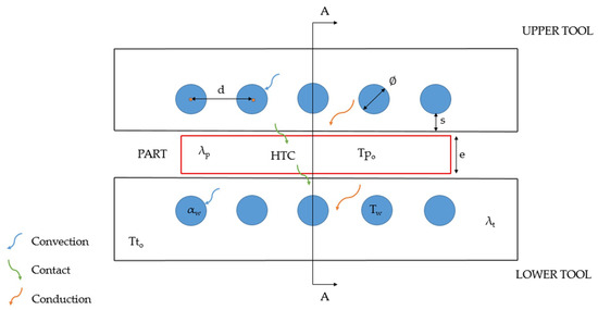
Figure 1. Scheme of a hot stamping tool with an upper cooled tool, a lower cooled tool, and a hot stamped part in between.

An overview of each variable employed is presented in the following section.

2.1. Cycle Time: Cooling Time (t₁)

The cycle time is a key parameter for all industrial production processes. As previously mentioned, the mechanical properties of the hot stamped parts are directly correlated with the cycle time and part temperature after cooling [14]. The hot stamping cycle time is defined in Figure 2.

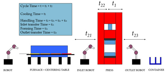
Figure 2. Scheme of a hot stamping line, where the cycle time components are defined.

The handling time (t₂) depends on the hot stamping line characteristics and the robot system. To simplify the DOE, the handling time (t₂) was taken as a constant value of 10 s.

However, two different cooling time (t₁) values (4 s and 10 s) were considered.

2.2. Part Material: Thickness (e) and Part Initial Temperature before Forming (Tp_o)

Part material 22MnB5, which is the most widespread steel in the hot stamping field, was selected for analysis. The physical properties for the material model are shown in Table 1.

Table 1. Relevant physical properties of the 22MnB5 steel at room temperature.

Symbol	Property	Value	Units
λp	Part thermal conductivity	21	W/m·K
Cpp	Part specific heat	550	J/kg·K
ρp	Part density	7850	kg/m3

The part thickness (e) and the part temperature after cooling under industrial production conditions are strongly correlated. The initial part temperature before forming (Tp_o) depends mainly on e, the furnace temperature, and the inlet transfer time [1,2]. If a high temperature is required for forming, due to the complexity of the hot stamping part, a faster transfer system (than the current system) can be installed. However, this increases the cost of the hot stamping line.

In the present work, e and Tp_o were selected as two of the studied parameters. Two values of e (1 mm and 3.5 mm) and Tp_o (700 °C and 850 °C) were chosen and targeted, respectively.

2.3. Cooling Design: Distance from the Cooling Channels to the Tool Surface (s) and Reduction Factor (β)

The design and efficiency of the cooling channels depend mainly on the channel diameter (∅), distance from the cooling channels to the tool surface (s), and distance between the channels (d) [1,2,4,5]. Thus, designing the maximum possible cooling channels for relatively thick parts is a good solution in terms of cooling, but increases the cost of the tool. Designing the tool with a short distance from the cooling channels to the tool surface increases the cooling effectiveness, but reduces the tool life. Therefore, knowledge of the relationship between each parameter and the part temperature after cooling under industrial production conditions is critical to effective tool design.

The ∅ and d values were accounted for by introducing a reduction factor (β) for the water convection factor (α_w) into the one-dimensional heat transfer model selected to build the DOE. This reduction factor was defined as follows:

$$\beta =\frac{\varnothing }{d}$$

(1)

The aforementioned s and β were chosen as working parameters. Two s values (6 mm, 12 mm) and two β values (0.3, 0.83) corresponding to ∅ values of 6 mm and 10 mm, and d values of 12 mm and 20 mm were calculated.

2.4. Heat Transfer Contact Factor (HTC)

The heat transfer contact factor (HTC) is one of the most important parameters, which defines the heat transfer between the hot stamped part and the tool [6,7,8,9,10]. This parameter affects part and tool temperatures after cooling under industrial production conditions. The press force (pressure) has a strong influence on the HTC [12].

The HTC increases with increasing pressure, leading to a decrease in the cycle time. A press with a relatively high force capacity has a cost effect in the hot stamping line.

Two values of the HTC (1500 W/m²·K and 2500 W/m²·K) were considered in this work.

2.5. Hot Stamping Tool: Material Conductivity (λ_t)

Tool material selection plays a key role in defining the cycle time of stamping tools. High thermal conductivity materials are a good option for reducing the cycle time, but a good balance between the λ_t, hardness, and steel price is essential. The physical values for the tool steel employed in the model are shown in Table 2.

Table 2. Physical values of hot stamping tool steel for dies and punches at room temperature.

Symbol	Property	Value	Value
Cpt	Tool specific heat	460	J/kg·K
ρt	Tool density	7800	kg/m3

The model also considered the tool initial temperature (Tt_o). To simplify the DOE, a constant Tt_o of 20 °C was set at the beginning of cycle 1.

In addition, the aforementioned λ_t was considered in the model, with two values (27 W/m·K and 45 W/m·K) employed during the study.

2.6. Cooling Water: Water Convection Factor (α_w)

A hot stamping line is composed of a furnace, a centering table, an inlet robot, a press, an outlet robot, a conveyor belt, and a chiller system. The water is heated during the hot stamping process, and enters the die through the cooling channels, removing the heat from the tool. This results in an increase in the water temperature, which is then reduced by cooling the water in the chiller (the reduction was essential for realizing a stable process). The chiller sets the initial temperature of the water. In this study, the water temperature during the cycle process was assumed to be constant. The water temperature (T_w) was set to 20 °C (see Table 3 for the physical properties of water in the model).

Table 3. Physical values of water at 20 °C.

Symbol	Property	Value	Units
µ	Water dynamic viscosity	0.001	Pa·s
k	Water thermal conductivity	0.5996	W/m·K
Cpw	Water heat capacity	4182	J/kg·K
ρw	Water density	998.3	kg/m3

In addition, the water convection factor (α_w) must be calculated. This coefficient is dependent on the Prandtl number, Reynolds number, and Nusselt number (Dittus and Boelter correlation), which are defined as follows:

Prandtl number (Pr):

$$\mathrm{Pr}=\frac{\mu ·C{p}_w}{k}$$

(2)

Reynolds number (Re):

$$Re=\frac{{\rho }_w·v·\varnothing }{\mu }$$

(3)

Nusselt number (Nu):

$$Nu=0.023·R{e}^{\frac{4}{5}}·P{r}^n$$

(4)

Water convection factor (α_w):

$${\alpha }_w=\frac{Nu·k}{\varnothing }$$

(5)

Two values (5000 W/m²·K and 15,000 W/m²·K) of α_w were employed.

2.7. Iterative One-Dimensional Heat Transfer Model

Industrial production conditions must be simulated for the formulation of an accurate formula corresponding to steady-state conditions. Therefore, 10 cycles of a one-dimensional heat transfer model were selected as the stabilization condition for the DOE. The model was then solved using a numerical method. The numerical methods for solving differential equations are based on replacing the differential equations with algebraic equations. In the case of the popular finite difference method, this is achieved by replacing the derivatives with differences. In the present work, the finite difference formulation of heat conduction is used for a section of the hot stamping tool, using the energy balance approach and solving the resulting equations per node. The energy balance method is based on subdividing the medium into a sufficient number of volume elements, and then applying an energy balance to each element. This energy balance is given as follows:

$$\dot{Q}cond, left+\dot{Q}cond,right+\dot{Q}conv,left+\dot{Q}conv,right+ \dot{Q}cont, left+ \dot{Q}cont, right+ \dot{E}gen= \frac{\Delta E}{\Delta t}$$

(6)

where $\dot{Q}cond$ is the rate of conduction heat, $\dot{Q}conv$ is the rate of convection heat, and $\dot{E}gen$ is the rate of generation heat inside the element.

The defined equations must be solved with a definite time increment (Δt). A Δt of 0.02 s was chosen to ensure convergence of the equations.

The model was defined in a section of a hot stamping tool, considering a symmetrical section in the middle of the part, as shown in Figure 3.

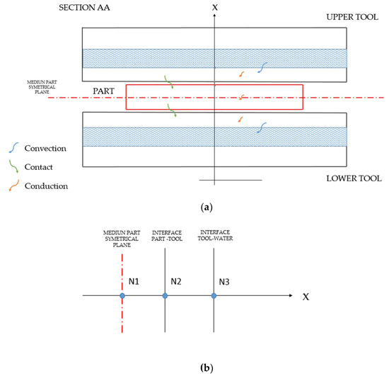
Figure 3. (a) Heat transfer model for a hot stamping tool. (b) Nodes for one-dimensional heat transfer model, with Node 1 (N1), Node 2 (N2), and Node 3 (N3).

The energy balance for each node is defined, and the equations for each temperature are formulated as follows.

The inside part temperature associated with t₁ corresponding to cycle number i ($\mathrm{Tipt}1{\mathrm{i}}_j$) in Node 1, within cycle i during increment j is found as

$$\mathrm{Tipt}1{\mathrm{i}}_j=\mathrm{Tipt}1{\mathrm{i}}_{j-1}+\left(\mathrm{Topt}1{\mathrm{i}}_{j-1}-\mathrm{Tipt}1{\mathrm{i}}_{j-1}\right)\ast \left(\frac{\lambda p\ast \Delta t}{\rho p\ast Cpp\ast \frac{e^2}{8}}\right)$$

(7)

The outside part temperature associated with t₁ corresponding to cycle number i ($\mathrm{Topt}1{\mathrm{i}}_j$) in part Node 2 within cycle i during increment j:

$$\mathrm{Topt}1{\mathrm{i}}_j=\mathrm{Topt}1{\mathrm{i}}_{j-1}+\left(\frac{\Delta t}{\rho p\ast Cpp\ast \frac{e}{2}}\right)\ast \left[\left(\mathrm{Tipt}1{\mathrm{i}}_{j-1}-\mathrm{Topt}1{\mathrm{i}}_{j-1}\right)\ast \frac{\lambda p}{e}+HTC\ast \left(\mathrm{Ttt}1{\mathrm{i}}_{j-1}-\mathrm{Topt}1{\mathrm{i}}_{j-1}\right)\right]$$

(8)

The tool temperature associated with t₁ corresponding to cycle i ($\mathrm{Ttt}1{\mathrm{i}}_j$) in tool Node 2, within cycle i during increment j:

$$\mathrm{Ttt}1{\mathrm{i}}_j=\mathrm{Ttt}1{\mathrm{i}}_{j-1}+\left(\frac{\Delta t}{\rho t\ast Cpt\ast \frac{s}{2}}\right)\ast \left[\left(\mathrm{Ttcht}1{\mathrm{i}}_{j-1}-\mathrm{Ttt}1{\mathrm{i}}_{j-1}\right)\ast \frac{\lambda t}{s}+HTC\ast \left(\mathrm{Topt}1{\mathrm{i}}_{j-1}-\mathrm{Ttt}1{\mathrm{i}}_{j-1}\right)\right]$$

(9)

The tool cooling channel temperature associated with t₁ corresponding to cycle i $(\mathrm{Ttcht}1{\mathrm{i}}_j$) in tool Node 3, within cycle i during increment j:

$$\mathrm{Ttcht}1{\mathrm{i}}_j=\mathrm{Ttcht}1{\mathrm{i}}_{j-1}+\left(\frac{\Delta t}{\rho t\ast Cpt\ast \frac{s}{2}}\right)\ast \left[\left(\mathrm{Ttt}1{\mathrm{i}}_{j-1}-\mathrm{Ttcht}1{\mathrm{i}}_{j-1}\right)\ast \frac{\lambda t}{s}+\left(\mathrm{Tw}-\mathrm{Ttcht}1{\mathrm{i}}_{j-1}\right)\ast \alpha w\ast \beta \right]$$

(10)

The tool temperature associated with t₂ corresponding to cycle i $(\mathrm{Ttt}2{\mathrm{i}}_j$) in tool Node 2, within cycle i during increment j:

$$\mathrm{Ttt}2i_j=\mathrm{Ttt}2{\mathrm{i}}_{j-1}+\left(\frac{\Delta t}{\rho t\ast Cpt\ast \frac{s}{2}}\right)\ast \left(\mathrm{Ttcht}2{\mathrm{i}}_{j-1}-\mathrm{Ttt}2{\mathrm{i}}_{j-1}\right)\ast \frac{\lambda t}{s}$$

(11)

Lastly, the tool cooling channel temperature associated with t₂ corresponding to cycle i ($\mathrm{Ttcht}2{\mathrm{i}}_j$) in tool Node 3, within cycle i during increment j:

$$\mathrm{Ttcht}2{\mathrm{i}}_j=\mathrm{Ttcht}2{\mathrm{i}}_{j-1}+\left(\frac{\Delta t}{\rho t\ast Cpt\ast \frac{s}{2}}\right)\ast \left[\left(\mathrm{Ttt}2{\mathrm{i}}_{j-1}-\mathrm{Ttcht}2{\mathrm{i}}_{j-1}\right)\ast \frac{\lambda t}{s}+\left(\mathrm{Tw}-\mathrm{Ttcht}2{\mathrm{i}}_{j-1}\right)\ast \alpha w\ast \beta \right]$$

(12)

The sub-index i refers to the correlative hot stamping stroke from 1 to 10. The sub-index j refers to the number of increments calculated from 1 to $\frac{t1}{\Delta t}$ or $\frac{t2}{\Delta t}$. The iterative diagram (see Figure 4) has been employed to ensure attainment of industrial production conditions.

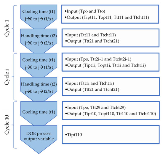
Figure 4. Iterative one-dimensional heat transfer model.

The inside part temperature associated with t₁ corresponding to cycle number 10 (Tipt110) will be analyzed for each run as a process output variable in the DOE.

2.8. Design of Experiments

The DOE was chosen to be a two-level factorial design (default generators) created with MINITAB ® software version 17 (Minitab Inc., State College, PA, USA), and the effects of eight factors were considered (see Table 4 for these factors and their corresponding levels).

Table 4. Values of the design of experiments (DOE) factors.

Factor		Level −1	Level +1	Units
s	Distance from channel to tool contact surface	6	12	mm
e	Part thickness	1	3.5	mm
λt	Tool thermal conductivity	27	45	W/m·K
αw	Water convection factor	5000	15,000	W/m2·K
HTC	Heat transfer contact factor	1500	2500	W/m2·K
t1	Cooling time	4	10	s
Tpo	Part initial temperature	700	850	°C
β	Reduction coefficient	0.3	0.83	n/a

A 2^8-1 fractional factorial design was selected, and therefore this study is a 128-run factorial design. As seen in Figure 5, the selected resolution for this project is VIII. This resolution ensures that no main effects or two-factor interactions are aliased with any other main effects or two-factor interactions. Moreover, this resolution ensures that no two-factor interactions are aliased with either three-factor interactions or four-factor interactions.

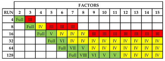
Figure 5. Different available resolutions.

2.9. Validation Testing

The experimental setup employed for determining the accuracy of the model is analogous to the one described in [12]. The specific conditions employed in this work are described as follows:

-

Test sample: 80 mm × 90 mm samples of a 3 mm thick (e), AlSi-coated 22MnB5 steel were conditioned by means of electric discharge machining (EDM). A 1.15 mm diameter × 30 mm deep hole was machined in the center of the sheet thickness and aligned with the axis of symmetry corresponding to the 90 mm long side of the samples. An AISI 316L sheathed Type K thermocouple 1 mm in diameter was inserted into the EDM hole up to the point where the tip of the thermocouple touched the bottom of the hole. The thermocouple was fixed in this position using a refractory adhesive.

-

Test tooling: a flat stamping tool with a 150 mm × 150 mm active surface. A QRO90 material in the quench and tempered condition (52 HRC, material conductivity (λ_t) = 33 W/m·K) was selected for the tools. The cooling channel design followed the “10–10–10” rule: 10 mm channel diameter (∅), 10 mm distance to surface (s), and 10 mm distance between channels (d).

-

Cooling intake conditions: water temperature (T_w) of 20 °C was used with a flow rate of 20 L per min to obtain a maximum water convection factor (α_w) of 15,000 W/m²·K; a lower factor can be obtained by regulating the water intake valve closure. Regulation down to 7500 W per m²·K was performed.

-

Press: the tests were performed in an MTS 180 hydraulic press (Materials Testing System, Eden Prairie, MN, USA). A four-step press stroke of 17 mm was programmed:

○

Step 1: rapid approximation speed of 34 mm/s up to a preload of 500 N.

○

Step 2: load increase up to 10 MPa at a rate of 1 mm/s to obtain an HTC of 2500 W/m²·K.

○

Step 3: 10 s of cooling time with fixed position control.

○

Step 4: sample release and a 34 mm/s rate to initial press position.

-

Tool temperature (Tt) measurement: combined thermography and direct-contact Type K thermocouples were used immediately after removing the press hardened sheet sample from the tool.

-

Heating and transfer time: austenitizing of the 22MnB5 samples was performed in a N7/H furnace (Nabertherm GmbH, Bahnhofstr. 20, Lilienthal, Germany) at a setpoint temperature of 900 °C. The furnace was preheated to this temperature, and samples were introduced for 300 s. The part initial temperature prior to forming (Tp_o) lies between 820 °C and 850 °C. Furthermore, after this dwell time, the austenitized samples were manually transferred to the press in ~4 s, i.e., from the opening of the furnace to the delivery of the sample inside the tooling. The final part was transferred from the tool to the conveyor in ~6 s. The total handling time (t₂) was ~10 s.

-

Cooling time (t₁): 10 s.

-

The test is performed with the same parameters for 10 cycles to achieve steady-state conditions equivalent to industrial production.

3. Results

3.1. Effects and Interaction Grade 2 of the Design of Experiments Factors

Different figures were developed as DOE results, in order to select the most important factors that affect the inside part temperature associated with t₁, corresponding to cycle number 10 (Tipt110). In Figure 6, the main effect of the different factors is visualized, and the relevance of this temperature is assessed.

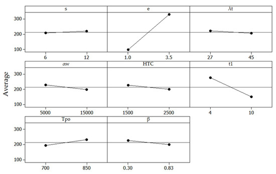
Figure 6. Main effect chart for Tipt110.

In Figure 7, the main interactions of the different factors can be visualized in order to assess the relevance of the inside part temperature associated with t₁, corresponding to cycle number 10 (Tipt110).

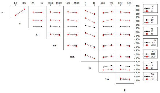
Figure 7. Main interaction chart for Tipt110.

The significant and insignificant effects and interactions (up to grade 2) affecting the inside part temperature associated with t₁ corresponding to Tipt110 can be visualized through a normal graph of standardized effects (see Figure 8).

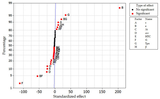
Figure 8. Normal graph of standardized effects.

In Figure 9, the Pareto chart of standardized effects can be visualized, with the most important effects and interactions up to grade 2 affecting the inside part temperature characterized by t₁ corresponding to Tipt110.

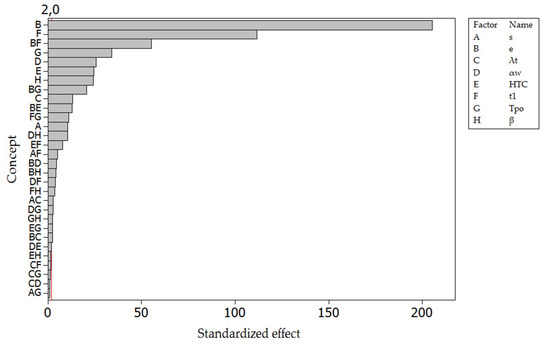
Figure 9. Normal graph of standardized effects.

3.2. Selected Effects and Interaction Grade 2 of the Design of Experiments Factors

For the sake of simplicity, and to minimize the loss of accuracy, only the standardized effects above 10 effect values were considered during the formulation of the final equation.

A normal graph of selected standardized effects corresponding to the most relevant factors is shown in Figure 10.

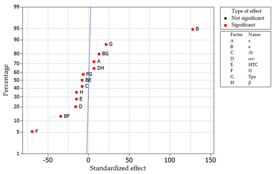
Figure 10. Normal graph of selected standardized effects.

The Pareto chart of the selected standardized effects can be visualized in the following plot (see Figure 11).

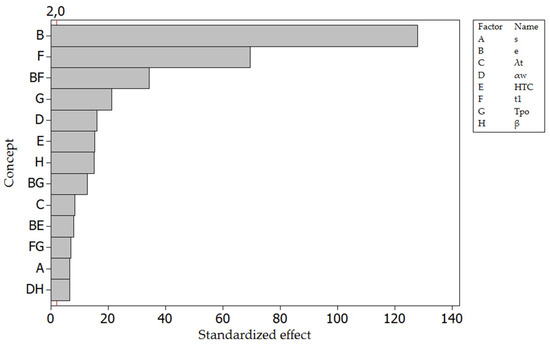
Figure 11. Normal graph of selected standardized effects.

Figure 12 shows the histogram of the residuals. The histogram reveals the absence of asymmetric data and outliers, reflecting the good accuracy of the factorial analysis.

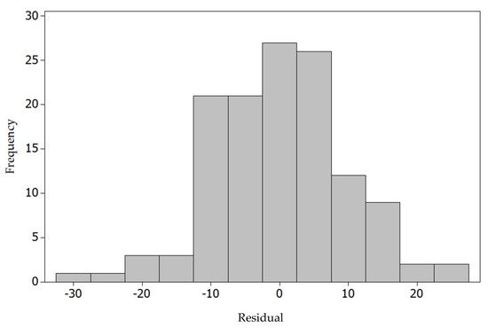
Figure 12. Histogram of residuals associated with selected standardized effects.

A plot of the residual versus size is shown in Figure 13. The lack of trends or patterns is indicative of independent residuals. The residuals in the graph fall randomly around the center line of asymmetry, indicating the good accuracy of the factorial analysis.

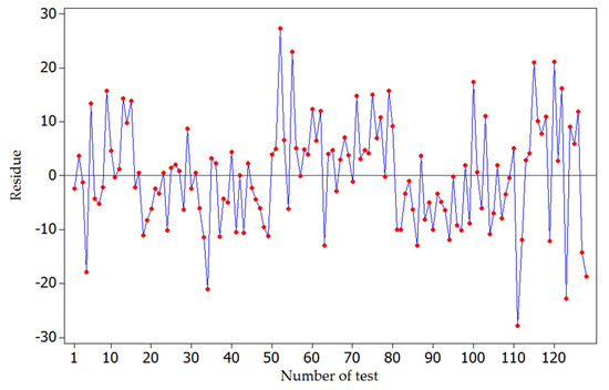
Figure 13. Residual vs size of selected standardized effects.

The formula for predicting the inside part temperature characterized by t₁ corresponding to cycle number 10 (Tipt110), with selected standardized effects, is given as follows:

$$Tipt\mathit{110}=C_1+C_2\ast e+C_3\ast t_1+C_4\ast \left(e\ast t_1\right)+C_5\ast T{p}_O+C_6\ast {\alpha }_w+C_7\ast HTC+C_8\ast \beta +C_9\ast \left(e\ast T{p}_O\right)+C_{10}\ast {\lambda }_t+C_{11}\ast \left(e\ast HTC\right)+C_{12}\ast \left(t_1\ast T{p}_O\right)+C_{13}\ast s+C_{14}\ast \left({\alpha }_w\ast \beta \right)$$

(13)

The constants for this equation are summarized in Table 5.

Table 5. Values of the equation constants.

Constant	Value
C1	−12.2034
C2	95.3917
C3	19.1345
C4	−8.28125
C5	0.172715
C6	−0.00541675
C7	−0.0031
C8	−95.6037
C9	0.123083
C10	−0.827257
C11	−0.023025
C12	−0.0276736
C13	1.96615
C14	0.00445165

3.3. Equation for Calculating Cooling Time (t₁)

The formula for predicting the cooling time (t₁) with selected standardized effects was deduced from Equation (13), and is provided below. The constants for this equation are summarized in Table 5.

$$t1=\frac{Tipt\mathit{110}-(C_1+C_2\ast e+C_5\ast T{p}_O+C_6\ast {\alpha }_w+C_7\ast HTC+C_8\ast \beta +C_9\ast \left(e\ast T{p}_O\right)+C_{10}\ast {\lambda }_t+C_{11}\ast \left(e\ast HTC\right)+C_{13}\ast s+C_{14}\ast \left({\alpha }_w\ast \beta \right))}{C_3+C_4\ast e+C_{12}\ast T{p}_O}$$

(14)

3.4. Test Validation

To verify the validity of the prediction model, the experimental setup described in the Materials and Methods section was tested, and the results were compared with predictions obtained via the simplified formulae. A force–time and temperature–time curve from the tests is shown in Figure 14. In this case, a cycle time of 10 s was programmed in the press, and the expected exit temperature in the steel sheet was calculated with the model. The thermocouple temperature was overlaid on the pressure curve for the two testing conditions shown in Table 6. Test 1 and Test 2 were distinguished by modifying the respective initial Tp₀ temperatures, and changing the water intake to the cooling channels.

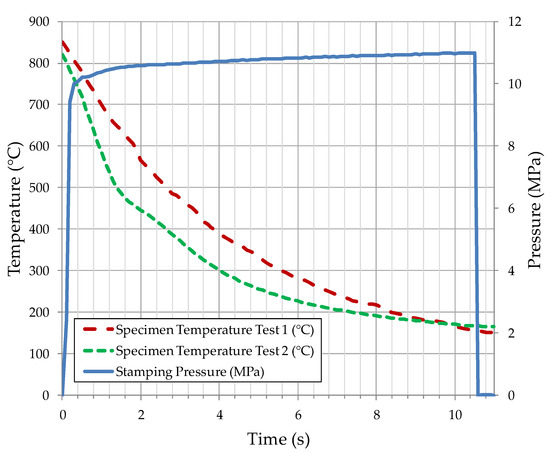
Figure 14. Test curves for verifying the model accuracy.

Table 6. Experimental checking of the accuracy characterizing the simplified polynomial for predicting Tipt110.

Process Factor		Test 1	Test 2	Units
s	Distance from channel to tool contact surface	10	10	mm
e	Part thickness	3	3	mm
λt	Tool thermal conductivity	33	33	W/m·K
αw	Water convection factor	15,000	7500	W/m2·K
HTC	Heat transfer contact factor	2500	2500	W/m2·K
t1	Cooling time	10	10	s
Tpo	Part initial temperature	850	820	°C
β	Reduction coefficient	0.5	0.5	n/a
Tipt110	Predicted temperature Measured temperature Deviation	159	175	°C
		150	165	°C
		+9	+10	°C

Equation (13) yielded an output temperature of 159 °C for Test 1 and 175 °C for Test 2 of the steel sheet. These values lie within 10 °C of the actual measured temperatures (150 °C and 165 °C for Test 1 and Test 2, respectively), corresponding to a deviation of <6% in the estimation of the cooling capacity. The accuracy of the proposed formulae depends on the accuracy of the finite difference modeling that was employed for the DOE, and thus, the prediction is inherently less accurate than an experimental DOE. Nevertheless, the time and resource investment required for an experimental DOE is significantly higher than that required for a finite difference-based one, and the accuracy to effort trade-off is considered satisfactory.

The experimental process variables selected for checking the simplified model lie between the Level −1 and Level +1 values that were chosen for the DOE (except for HTC and cooling time). Therefore, the checked results indicate that interpolation between these levels had only a slight effect on the predicted trends.

4. Conclusions

In light of the results, a reasonable trade-off between accuracy and ease of calculation is achieved by the application of a DOE, which combines the results of a complex iterative finite difference calculation method into a straightforward equation. The proposed equation, which allows cycle-time estimation via simple algebraic calculations, has been checked against a real laboratory case study. This case, which is located inside the interpolation window of the DOE, has yielded very similar results to the predictions from Equation (14). The DOE has proved to be a powerful simplification tool for hot stamping cycle-time calculation. The differential equations used as the basis for the DOE are reduced to a simple second-order polynomial that can be resolved in a straightforward manner. The conclusions of the present work can be summarized as follows:

-

The proposed simplified formula offers excellent fitting with experimental results in interpolation scenarios.

-

Provided that most industrial hot stamping processes are contained in the process window enclosed by the DOE variables, the proposed simplified formula can be applied extensively for a first approach to cycle-time calculation.

Nevertheless, no extrapolation is recommended for the model, as several limitations would be introduced when real geometries are considered. Moreover, the tool and cooling channel geometries have been considerably simplified. The method is, in general, considered to be a good solution for a first approach in part-cost assessment, which supports rapid feedback during the development of a new component. For accurate productivity studies, finite element methods will still be required during a detailed study of the component. The accuracy assessment, both for the proposed DOE model and for finite element methods, should include also an r-square model accuracy test against a representative set of experimental data.

References

- Karbasian, H.; Tekkaya, A.E. A review on hot stamping. J. Mater. Process. Technol. 2010, 210, 2103–2118. [Google Scholar] [CrossRef]
- Mori, K.; Bariani, P.F.; Behrens, B.-A.; Brosius, A.; Bruschi, S.; Maeno, T.; Merklein, M.; Yanagimoto, J. Hot stamping of ultra-high strength steel parts. CIRP Ann. Manuf. Techn. 2017, 66, 755–777. [Google Scholar] [CrossRef]
- Cortina, M.; Arrizubieta, J.I.; Calleja, A.; Ukar, E.; Alberdi, A. Case study to illustrate the potential of conformal cooling channels for hot stamping dies manufactured using hybrid process of laser metal deposition (LMD) and milling. Metals 2018, 8, 102. [Google Scholar] [CrossRef]
- He, B.; Ying, L.; Li, X.; Hu, P. Optimal design of longitudinal conformal cooling channels in hot stamping tools. Appl. Therm. Eng. 2016, 106, 1176–1189. [Google Scholar] [CrossRef]
- Lee, S.H.; Park, J.; Park, K.; Kweon, D.K.; Lee, H.; Yang, D.; Park, H.; Kim, J. A study on the cooling performance of newly developed slice die in the hot press forming process. Metals 2018, 8, 947. [Google Scholar] [CrossRef]
- Gorriño, A.; Angulo, C.; Muro, M.; Izaga, J. Investigation of thermal and mechanical properties of quenchable high-strength steels in hot stamping. Metall. Mater. Trans. B 2016, 47, 1527–1531. [Google Scholar] [CrossRef]
- Caron, E.J.F.R.; Daun, K.J.; Wells, M.A. Experimental heat transfer coefficient measurements during hot forming die quenching of boron steel at high temperatures. Int. J. Heat Mass Tran. 2014, 71, 396–404. [Google Scholar] [CrossRef]
- Abdulhay, B.; Bourouga, B.; Dessain, C. Thermal contact resistance estimation: Influence of the pressure contact and the coating layer during a hot forming process. Int. J. Mater. Form. 2012, 5, 183–197. [Google Scholar] [CrossRef]
- Mendiguren, J.; Ortubay, R.; Saenz de Argandoña, E.; Galdos, L. Experimental characterization of the heat transfer coefficient under different close loop controlled pressures and die temperatures. Appl. Therm. Eng. 2016, 99, 813–824. [Google Scholar] [CrossRef]
- Salomonsson, P.; Oldenburg, M.; Akerström, P.; Bergman, G. Experimental and numerical evaluation of the heat transfer coefficient in press hardening. Steel Research Int. 2009, 80, 841–845. [Google Scholar] [CrossRef]
- Chang, Y.; Tang, X.; Zhao, K.; Hu, P.; Wu, Y. Investigation of the factors influencing the interfacial heat transfer coefficient in hot stamping. J. Mater. Process. Technol. 2016, 228, 25–33. [Google Scholar] [CrossRef]
- Muro, M.; Artola, G.; Gorriño, A.; Angulo, C. Effect of the martensitic transformation on the stamping force and cycle time of hot stamping parts. Metals 2018, 8, 385. [Google Scholar] [CrossRef]
- Wang, L.; Zhu, B.; Wang, Y.; An, X.; Wang, Q.; Zhang, Y. An online dwell time optimization method based on parts performance for hot stamping. Procedia Eng. 2017, 207, 759–764. [Google Scholar] [CrossRef]
- Muvunzi, R.; Dimitrov, D.M.; Matope, S.; Harms, T.M. Development of a model for predicting cycle time in hot stamping. Procedia Manuf. 2018, 21, 84–91. [Google Scholar] [CrossRef]
- Del Pozo, D.; López de Lacalle, L.N.; López, J.M.; Hernández, A. Prediction of press/die deformation for an accurate manufacturing of drawing dies. Int. J. Adv. Manuf. Technol. 2008, 37, 649–656. [Google Scholar] [CrossRef]
- Nakagawa, Y.; Mori, K.; Maeno, T. Springback-free mechanism in hot stamping of ultra-high-strength steel parts and deformation behavior and quenchability for thin sheet. Int. J. Adv. Manuf. Technol. 2018, 95, 459–467. [Google Scholar] [CrossRef]
- Gaitonde, V.N.; Karnik, S.R.; Davim, J.P. Taguchi multiple-performance characteristics optimization in drilling of medium density fibreboard (MDF) to minimize delamination using utility concept. J. Mater. Process. Technol. 2008, 196, 73–78. [Google Scholar] [CrossRef]
- Coelho, R.T.; de Souza, A.F.; Roger, A.R.; Rigatti, A.M.Y.; Ribeiro, A.A.L. Mechanistic approach to predict real machining time for milling free-form geometries applying high feed rate. Int. J. Adv. Manuf. Technol. 2010, 46, 1103–1111. [Google Scholar] [CrossRef]
© 2019 by the authors. Licensee MDPI, Basel, Switzerland. This article is an open access article distributed under the terms and conditions of the Creative Commons Attribution (CC BY) license (http://creativecommons.org/licenses/by/4.0/).