Abstract
On the basis of the Volume Correlation Model (VCM) as well as data on steel consumption and scrap collection per industry sector (construction, automotive, industrial goods, and consumer goods), it was possible to estimate service lifetimes of steel in the United States between 1900 and 2016. Input data on scrap collection per industry sector was based on a scrap survey conducted by the World Steel Association for a static year in 2014 in the United States. The lifetimes of steel calculated with the VCM method were within the range of previously reported measured lifetimes of products and applications for all industry sectors. Scrapped (and apparent) lifetimes of steel compared with measured lifetimes were calculated to be as follows: a scrapped lifetime of 29 years for the construction sector (apparent lifetime: 52 years) compared with 44 years measured in 2014. Industrial goods: 16 (27) years compared with 19 years measured in 2010. Consumer goods: 12 (14) years compared with 13 years measured in 2014. Automotive sector: 14 (19) years compared with 17 years measured in 2011. Results show that the VCM can estimate reasonable values of scrap collection and availability per industry sector over time.
1. Introduction
Information on the lifetime of products and applications is important to evaluate the availability of recyclable metals. The metal contained in products and applications becomes available as scrap at the end of product life. Metal scrap reserves are a substitute for natural resources (iron ore) that are used for ironmaking and steelmaking. By optimizing the collection of recyclable metals, it is possible to preserve natural resources, save energy, and lower the CO2 emissions associated with steelmaking [1].
The availability of recyclable metals can be estimated with empirical survey-based methods or with model-based methods. The model-based methods are referred to as dynamic material flow models (DMFMs) and are based on both the inflow and outflow of metals as well as the lifetime of products and applications in society [2,3,4,5,6,7,8]. Product lifetimes can be obtained from surveys of products and applications; lifetimes can be estimated with the Volume Correlation Model (VCM), a model-based method.
Surveys of measured lifetimes have been published for product groups such as household appliances, automotive and transportation applications, buildings, and bridges [9,10,11,12,13,14,15,16,17,18]. These studies have been published by bodies such as NACE International, U.S. Department of Transport (National Bridge Inventory), Nevada Department of Taxation, U.S. Department of Commerce, National Association of Home Builders, U.S. Army Corps of Engineers, U.S. Department of Transportation, and Amtrak. An overview of the reported lifetimes of products in the U.S. is given in Appendix A [9,10,11,12,13,14,15,16,17,18], which is summarized in Table 1. These analyses are based on the average age of products in-use and depreciation periods and do not state the steel tonnages in the products.

Table 1.
Previously reported average lifetimes of steel by industry sector and product groups in the U.S. between 1925 and 2014.
Another model-based method to estimate the lifetime of products and applications is the Volume Correlation Model (VCM) [19,20,21,22,23]. The VCM estimates the in-use lifetime of steel. Two different lifetimes are calculated: the scrapped and apparent lifetimes (previously termed “true” and “full” lifetimes) [19,20,21,22,23]. The scrapped lifetime corresponds to the service lifetime, similar to the average in-use lifetime of steel estimated with empirical survey-based studies.
The VCM relies on annual data on steel consumption and scrap collection. Because end-of-life (EOL) products are normally not identified by origin or application, information on scrap collection per industry sector is not generally available [24]. In this study, scrap collection per industry sector in the United States was estimated from a scrap survey conducted by the World Steel Association for the year 2014 (see Appendix B) [25]. The sectors considered were construction, appliances, industrial goods, and automotive products. The survey accounted for approximately 29% of all scrap collected in the U.S. in 2014 and was assumed to be representative. In this work, the results of the scrap survey were extrapolated from zero recycling to the 2014 values for the period 1900 to 2016. Steel consumption per industry sector for this period (1900 to 2016) was based on an analysis conducted by the World Steel Association [26].
In this study, it was investigated whether it was possible to verify the input data on scrap collection per industry sector between 1900 and 2016 based on the VCM method. More specifically, this study (1) investigated the use of the VCM method to estimate the service lifetimes of steel in the US by industry sector on an annual basis and (2) compared model results with lifetime measurements of products and applications in the US. The VCM results (calculated steel lifetimes) for the US were also compared with calculated lifetimes for Sweden and the world between 1900 and 2010.
2. Input Data
2.1. Scrap Collection
The input data of the VCM are the tonnages of steel consumption and scrap collection for the construction, industrial goods, automotive, and consumer goods (appliances) sectors. A simple material flow chart of steel is shown in Figure A1 (see Appendix C). Scrap collection in the United States was estimated according to U.S. Geological Survey (USGS) data [27]. Total collected steel scrap in the US was calculated based on reported scrap consumption in ironmaking and steelmaking, scrap exports and imports, and subtracting internal scrap (years 1938 to 2016). For the years 1900 to 1934, there were no data available for the reported scrap consumption and an approximate mass balance was used instead, as follows: Total raw material usage per ton of crude steel production between 1934 and 1954 was assumed to have been the same from 1900 to 1933. Raw material usage includes scrap consumption, the iron content in the apparent consumption of iron ore (including iron ore used to produce direct reduced iron), and the net trade of pig iron. The average mass ratio of total metal usage to crude steel production was calculated to have been 1.28 between 1934 and 1954. This time base was used because the ratio appeared to be constant during this period. The mass ratio of total scrap usage to crude steel production was estimated by subtracting the iron content in the reported consumed iron ore and the net use of pig iron in crude steel production between 1900 and 1933 (yielding a ratio of 0.74). The resulting estimated mass ratio of scrap consumption (home and purchased scrap) to crude steel production was 0.54. Variations in the accuracy of this necessary approximation would not significantly affect the overall calculation because the tonnage of steel consumed in the period 1900–1933 was small compared with the overall period (see Figure 2).
The purchased steel scrap tonnages for the years 1905 to 1933 were taken from USGS data and the values were extrapolated to 4 M ton in 1900 [28]. The internal scrap was then estimated by subtracting the purchased steel scrap from total scrap usage. Half of the purchased steel scrap was assumed to be obsolete scrap for the years 1900 to 1955. Prompt steel scrap values were taken from a Nathan Associates report covering the years 1956 to 2009 [29]. According to the USGS report, internal scrap also included obsolete scrap from old steel plant equipment and buildings, which amounted to approximately 2% of scrap in 1980 and in 2014 [27]. The obsolete scrap tonnage was subtracted from the internal scrap tonnage by using the same ratio of 0.02 (fraction of internal scrap that is obsolete scrap) for the period 1900 to 2014. Consumption of old scrap at foundries was estimated from a 36% ratio of scrap usage to total casting production between 1972 and 2013 [27]. The total domestic steel scrap collection was the sum of purchased steel scrap at steel mills, scrap consumption at foundries, and exports, from which imported steel scrap was then subtracted [27].
Prompt steel scrap is generated when the finished steel from steel mills and foundries is used to fabricate products at other facilities. Prompt steel scrap was included in the total calculation for steel products and for steel scrap collection. Theoretically, adding this mass to steel consumption and to scrap collection should not significantly affect the model results. Prompt steel scrap was calculated to be 27% of the total scrap collection in 2014 in the U.S., based on the World Steel Association scrap survey [25]. This ratio was similarly calculated to be 26% in 2009 in the US according to a separate study performed by Nathan Associates [29].
Scrap collection per industrial sector was estimated according to the 2014 scrap survey conducted by the World Steel Association [25]; see Table 2 and Appendix B. The proportion of scrap originating from the four sectors was assumed to be equal to the 2014 values for the years 2011 to 2016. In the absence of other information, the ratios were extrapolated to earlier years (see Figure 1a). The proportion of scrap from consumer goods was assumed to increase from 0.05% in 1931 to 0.6% in 1944, subsequently increasing to 11.5% in 2011. The relative contribution from the automotive sector was assumed to increase from 0.001% in 1911 to 1.7% in 1944 and then to 31.7% in 2011. The assumed increase in automotive scrap collection after 1944 appears reasonable on the basis of the following: (1) the relatively low consumption of steel by these sectors in earlier years (see Figure 2), and (2) the reported history of automotive recycling, with shredders having only been widely available from the 1950s as well as “graveyards” of automobile hulks persisting until the 1970s [30]. The small “tails” before 1945 for automotive and consumer goods were added to reduce edge effects (discussed below).
Table 2.
Relative contribution of scrap from different industry sectors to obsolete steel scrap collection for the year 2014. Results of the scrap survey [25] and adjusted values used as input data in the calculations.
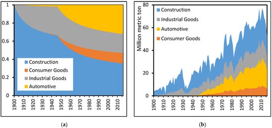
Figure 1.
Input data on U.S. scrap collection by industry sector between 1900 and 2016: (a) ratios of scrap collected and (b) tonnages of scrap collection.

Figure 2.
Input data on U.S. steel consumption by industry sector between 1900 and 2016: (a) ratios of relative steel consumption per industry sector and (b) tonnages of steel consumed.
The proportion of scrap from industry goods was assumed to increase from zero before 1900 to 31.4% in 1945 and then decrease to 21.1% in 2011. The assumed zero ratio before 1900 for industry goods appears reasonable based on the rapid industrial development during the late 1800s and early 1900s, when new technologies and specialized machines replaced manual work. Examples include (1) the implementation of large scale factories with new standardized production methods and (2) the upscaling in farming due to new agricultural technology such as the mechanical reaper [31].
The relative scrap collection per industry sector (from the World Steel Association scrap survey; see Table 2) was adjusted slightly to achieve better agreement with the lifetime values in Table 1. The largest change was for consumer goods. It appears that the scrap survey overestimated the contribution of this sector, or that the World Steel Association analysis underestimated the consumption by this sector. Using these values as-is would have resulted in a recycling rate greater than 100% (the calculations for which are presented below; see Figure 5). Figure 1b shows the estimated tonnage of steel scrap from the four sectors based on the estimates of obsolete scrap collected and of the relative contributions of the different sectors. Figure 1a shows the ratios of scrap collection per industry sector between 1900 and 2016. These ratios were assumed to be representative for the total steel scrap collection in the U.S. including prompt steel scrap.
Figure 1 and Figure 2 show large variations in steel consumption and scrap collection, with the business cycles lasting several years. The scrap collection rate follows the steel consumption rate, likely because of the sensitivity of scrap collection to price. Increased steel demand increases the scrap price, which increase the scrap collection rate [32]. Concurrently, steel consumption is highly sensitive to economic cycles [33]. Major economic events can be recognized in Figure 2, including the downturns of the 1930s and 2008–2009 as well as the rapid growth associated with the period 1940–1950. Over the century of data considered in this work, the share of consumption in the automotive and consumer-goods sectors has increased, while that of industrial goods has remained approximately constant.
2.2. Steel Consumption
The total steel consumption represents the net utilization of steel as finished products, including steel that was imported (as semi-finished or finished products as well as manufactured goods). The lifetime of steel was assumed to last from the start of utilization as a finished product until collection and processing into recyclable scrap (ready for use in steel mills and foundries).
Steel consumption in the United States was calculated from USGS data [27] as the sum of apparent finished steel consumption between 1900 and 2016 as well as foundry shipments between 1972 and 2016 (adjusted for exports and imports). No earlier data on foundry shipments were available. The average foundry shipments were, on average, 15% of the total shipments (from steel mills and foundries) for the years 1971 to 1981. The net indirect trade of steel in manufactured goods was taken from World Steel Association data for the years 1970 to 2016 [34,35]. The average net indirect trade of steel was calculated to be nine million metric tons per annum during the period, which made the U.S. a net importing country of steel in manufactured goods. Prompt steel scrap was included in the steel consumption because prompt scrap is generated after finished steel products have been shipped from steel mills and foundries.
Steel consumption ratios in the four industrial sectors in the U.S. were taken from World Steel Association data for the years 1900 to 2013 [9] and assumed to be the same for 2014–2016 as for 2013; see Figure 2a. The ratios were multiplied by the calculated total steel consumption to yield the estimated consumption by sector, shown in Figure 2b.
Figure 2b shows that, by far, the largest steel consumer in the U.S. was the construction sector, accounting for approximately 45–80% of the total steel consumption in US between 1900 and 2016. The remaining steel consumption in US in 2016 was in the automotive sector (25%), industry goods (20%), and consumer goods (10%).
3. Calculation Procedure
The model used in this study, the Volume Correlation Model (VCM), has been described in detail in other studies [19,20,21,22,23]. The model was implemented in Excel® spreadsheets in combination with MATLAB® [36,37]. The VCM can be used to evaluate the time difference between reported data on steel consumption and scrap collection. The model calculates the scrapped and apparent lifetimes of steel. The scrapped lifetime of steel is the (estimated) actual service lifetime of steel; the apparent lifetime is defined below.
In a previous study, the scrapped and apparent lifetimes of steel were calculated for Sweden and the world [19,20]. In this study, the lifetimes of steel were recalculated with Swedish and global steel data for 1900 to 2010, for direct comparison with the calculations for the U.S. as presented here.
The apparent lifetime is predominantly used to calculate moving averages of scrap recovery rates, as described below. The apparent lifetime is calculated by assuming full recovery (as scrap) of all steel in final products, i.e., every ton of steel that entered service as a finished product is assumed to be eventually recoverable as scrap. Clearly, this is not always the case, and incomplete recovery is considered when calculating the scrapped lifetime.
The apparent lifetime of steel (λapp) has been found as the time difference between a given year tx (with a known cumulative tonnage of scrap collected up to this time: the left term in the equation below) and the number of years (in the past) required to consume the same tonnage of steel:
In this expression, Δmscrap(t) is the mass of scrap collected during year t (years since 1900), Δmconsumed(t) is the total steel consumption in year t, and λapp is the apparent lifetime of steel. This expression is used to find the apparent lifetime (λapp).
Not all consumed steel is recycled. The apparent recovery rate η(t) is found as the ratio of steel recycled in a given year to the moving average steel consumption over a longer period, taken to be 2λapp.
At the beginning of the time period considered in the calculations, the time period (for averaging the recovery rate) could be longer than the input data available. For calculating the recovery rate, the moving average was instead calculated over the time period zero to t, in cases where 2λapp > t. For the input data used here, the shorter integration period was used for the first seven years of data for the automotive sector, four years for consumer goods, one year for the construction sector, and the first six years of industrial goods.
Given the long lifetime of steel, the non-recirculated amount of steel is a reserve that is potentially available for future collection. This reserve may become a loss if the steel is not collected after a significant time period. Since the annual apparent recovery rate is based on the moving average of steel consumption, it would not necessarily be equivalent to the recycling rate in any given year; however, the longer-term averages (weighted by tonnage of steel) of the apparent recovery rate and recycling rate would be equal. Using the (time-varying) recovery rate, the amount of potentially recyclable steel added from each year’s consumption is estimated as follows:
Here, potentially recyclable steel refers to previously consumed steel that has been recycled within an apparent lifetime of steel. The tonnage of recyclable steel depends not solely on the availability of a reserve of steel but also strongly on scrap price; this formulation helps to highlight this effect.
The scrapped lifetime of steel is calculated as the time difference (λscrapped) between a given year tx (with a known cumulative tonnage of scrap collected) and time required to have accumulated the same tonnage of potentially recyclable steel in products:
In this expression, λscrapped is the scrapped lifetime of steel. As Equation (4) shows, the principle suggests that the cumulative mass of scrap collected up to a given year equals a fraction (the recovery rate) of the steel used in products up to a specific date λscrapped years earlier. Use of an annual recovery rate (rather than a constant ratio) helps to account for some of the variations in scrap collection.
The integration period used to calculate the moving average steel consumption rate affects the results. The effect of the integration period arises, in part, from fluctuations in steel consumption and recycling (in response to economic cycles) as well as the increase in steel consumption over the period considered. To test the effect of the integration period, the scrapped lifetime for total steel in the U.S. for the years 1900 to 2016 was calculated based on three different integration periods: λapp, 2λapp, and 3λapp (as used in Equation (2)). The resulting calculated scrapped lifetimes of steel for the different integration periods are shown in Figure 3. The difference between the apparent lifetime and scrapped lifetime was larger with a shorter integration period. If this large difference were real, it would imply that a large proportion of the steel would be lost and never recycled, which does not appear to be realistic, given reported recycling rates. The results were also compared with weighted averages of the reported lifetime of steel (the box in Figure 3) for 2010–2015. The reported sector lifetimes (listed in Table 1) were weighted using either the relative amount of steel consumed by each sector (yielding an average lifetime of 29 years) or the relative amount of scrap recovered from each sector (yielding an average lifetime of 25 years). The proportions of steel consumed were as given in Figure 2 and scrap ratios as in Table 2. The calculated average lifetime was close to the scrapped lifetime of steel, calculated with 2λapp as the integration period. On the basis of these results, the integration period was chosen to be 2λapp.
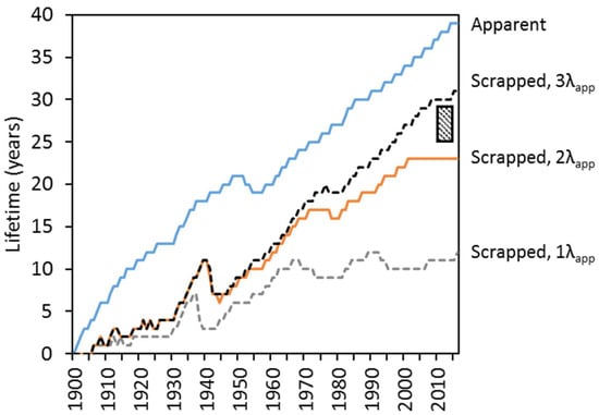
Figure 3.
The apparent lifetime of all steel consumed in the U.S., with the scrapped lifetime calculated with integration periods of λapp, 2λapp, and 3λapp. The shaded box shows the weighted average of the reported lifetime of steel for 2010–2015.
4. Results and Discussion
4.1. Calculated Lifetimes per Industry Sector in the U.S.
Calculated annual steel consumption and scrap collection tonnages per industry sector in the U.S. between 1900 and 2016 are shown in Figure 4, with apparent recovery rates in Figure 5. On the basis of the low recovery rate, the construction sector had the largest tonnage of non-recirculated steel, with approximately 55% of the total steel consumption collected within the apparent lifetime of steel. The results also show that the apparent recovery rate could temporarily be above 100%, as seen in Figure 4b–d, in years when the tonnage of steel scrap collected was larger than the moving average tonnage of steel produced. In those years, scrap was collected from accumulated scrap reserves. From simple mass balance considerations, the weighted average apparent recovery rate cannot be greater than 1 (100% recovery) over time. However, for all sectors apart from construction, the apparent recovery rate was close to 1, resulting in similar scrapped and apparent lifetimes and indicating low losses of unrecycled steel from the system (see Figure 5b–d).
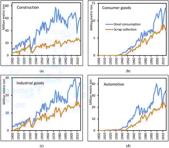
Figure 4.
Input data on steel consumption and scrap collection for the following industry sectors: (a) construction, (b) consumer goods, (c) industry goods, (d) automotive sector between 1900 and 2016 in the U.S.

Figure 5.
Apparent recovery rates of steel per industry sector in the U.S. between 1900 and 2016: (a) construction, (b) consumer goods, (c) industry goods, and (d) automotive sector.
The end-of-life recycling rate (EOL-RR) of metals is defined as the ratio of the tonnage of old steel scrap collected to the steel tonnage in EOL products [38]. A 2011 United Nations Environment Programme report on the EOL-RR of steel in different countries showed the value to be between 70% and 90% [38]. In a USGS study, the EOL-RR of steel in the U.S. in 1998 was calculated to be 47%, taking the lifetime of steel as 19 years [39]. In the present study, the collected steel scrap included both old scrap and prompt scrap. Although the calculated apparent recovery rates fluctuated due to the input data, the longer-term average appeared to be constant and similar to the previously reported EOL-RR. In this work, the average apparent recovery rate for the years 1998 to 2010 for total steel in the U.S. was calculated to be 73%, with a lowest value of 69% and a highest value of 83%, similar to the values of the end-of-life recycling rate quoted above.
The calculated scrapped and apparent lifetimes of steel per industry sector in the U.S. between 1900 and 2016 are shown in Figure 6a–d. For comparison, the figure includes data on measured in-use lifetimes of products and applications in the U.S. over certain periods; these are shown as individual data points or ranges of measure lifetime and period of measurement (lines and boxes). These measured lifetimes are also summarized in Table 1.
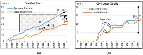

Figure 6.
The scrapped and apparent lifetimes of steel in the U.S. between 1900 and 2016 calculated with the Volume Correlation Model (VCM), compared with previously reported lifetime measurements of steel products in-use in the U.S. (literature values are shown as filled circles for single years and boxes for studies referring to multiple years, with reference numbers indicated): (a) construction, (b) consumer goods, (c) industrial goods, and (d) automotive sector.
The scrapped (and apparent) lifetimes of end-of-life steel products in 2016 in the U.S. were calculated to be as follows: a scrapped lifetime of 30 years (apparent lifetime, 53 years) for the construction sector; 17 (28) years for industrial goods; 17 (21) years for the automotive sector; and 13 (15) years for consumer goods.
The results show edge effects at the beginning of the calculation period for the automotive and consumer goods sectors, resulting in a peak in the calculated scrapped and apparent lifetimes (marked in Figure 6b,d). These edge effects stemmed from an inconsistency between the input data on steel consumption and scrap collection and resulted in part from the assumption that scrap was increasingly collected from these sectors from 1945. This appeared to cause the calculated lifetime of steel at the start of the period of substantial scrap collection to be excessively large, resulting in a peak in the calculated lifetime of steel. However, the peak might be real. In the absence of large-scale recycling, older scrap would have accumulated before 1945. It does not appear to be possible to test this calculation with the available data. Although the in-use lifetime of automobiles did not change for automobiles that were deregistered over this period [40], the time lapse between deregistration and recycling (for this period) is not known.
A similar but less obvious effect applies to the calculated lifetimes of steel construction and industrial goods, at the start of the period considered (from 1900 onwards). The scrapped lifetime is incorrectly shown as zero. This inevitably arose from the arbitrary choice of a starting date, subject to the limitations of the available data. However, for all sectors, the calculated scrapped lifetimes did correspond to the previously reported lifetimes for later years (Figure 6). Additionally, the calculated values at least fell within the rather wide range of reported lifetimes. On the basis of that agreement, the estimated lifetimes appeared to be reliable for 1950 onwards.
The average lifetime of steel generally showed an increasing trend for all sectors over the century of data considered, likely indicating that the quality of steel products has improved over time. The comparison between the model results and the lifetime measurements of steel showed that the calculated values based on the VCM were within the range of lifetime measurements of steel in the U.S. (Figure 6). Exceptions included two estimates of the lifetimes of steel in the industrial and consumer appliance sectors: the calculated lifetime (from the VCM in this work) was significantly shorter than the reported (measured) lifetime. However, these sectors cover a wide range of products (with a wide range of lifetimes, as indicated by Figure 6) and the disagreement may have simply reflected the difficulty of obtaining a representative sample when measuring in-use lifetimes.
4.2. The Lifetimes of Steel in the U.S., Sweden, and the World
The lifetime of steel (total for all sectors) was estimated with the VCM based on steel consumption and recycling in the U.S., Sweden, and the world between 1900 and 2010. The scrapped and apparent lifetimes of steel in the different regions are compared in Figure 7a,b. The estimated scrapped lifetime of steel was similar in all the regions, reflecting the global nature of steel markets. There were larger differences between the apparent lifetimes, especially around the middle of the 20th century. Since the difference between the apparent and scrapped lifetime was related to the recovery rate, these results indicate the relatively large proportions of non-recycled steel in the U.S. and the world. The estimated scrapped (and apparent) lifetimes of steel in 2010 were as follows: a scrapped lifetime of 32 years (apparent lifetime: 35 years) in Sweden, 29 (39) years on a global scale, and 23 (37) years in the U.S.

Figure 7.
Steel lifetimes (total for all sectors) in the U.S., Sweden and the world, calculated with the VCM for 1900 to 2010: (a) scrapped lifetime; (b) apparent lifetime.
5. Conclusions
The scrapped and apparent lifetimes of steel per industry sector in the U.S. were calculated on an annual basis for the years between 1900 and 2016, using the Volume Correlation Model (VCM) method. The calculated steel lifetimes were within the range of previously reported lifetime measurements for products and applications in all industry sectors. The apparent lifetime of steel varied between countries and between different industry sectors in the U.S. The difference between the scrapped and apparent lifetimes of steel was significant and should be considered when forecasting the availability of steel scrap based on Dynamic Material Flow Models (DMFMs). In previous DMFMs the lifetime of steel was based on lifetime measurements on products and applications [2,3,4,5,6,7,8]. On the basis of DMFMs, it is possible to estimate steel scrap generation at national and industry sector levels. The information on the availability of steel scrap per industry sector can assist in the planning of waste management and steelmaking facilities.
Supplementary Materials
The following data are available online at http://www.mdpi.com/2075-4701/8/5/338/s1, Excel document with input data and results.
Author Contributions
A.G. did the literature survey, data gathering and calculations, analyzed the data, wrote the paper; P.C.P. did literature survey, data gathering, analyzed the data, and wrote the paper.
Acknowledgments
The authors would like to thank the Swedish Steel Producers Association, the Hugo Carlssons Foundation, and the Axel Hultgrens Foundation for financial support of AG. The authors would also like to thank Carnegie Mellon University Libraries for its financial support for the publication fee.
Conflicts of Interest
The authors declare no conflict of interest.
Appendix A
Survey-based estimates of the in-use lifetime of products and applications in the United States.
Table A1.
Average lifetime per unit in the construction sector in the United States.
Table A1.
Average lifetime per unit in the construction sector in the United States.
| Product groups | References | Method | Timeline | Average Lifetime |
|---|---|---|---|---|
| American Housing Survey, General Housing Data, all Housing Units. | U.S. Census Bureau, Current Housing Reports, Series H150/11, American Housing Survey for the United States: 2011, Table C-01-AH. [9] | Lifetime of buildings used in Unites States | 2015 2013–2014 2011 | 39 years 44 years 42 years |
| American Housing Survey, General Housing Data, all Housing Units. | U.S. Department of Commerce. Bureau of Economic Analysis. Table A-1. Characteristics of the housing inventory 1973, 1980 and 1970 page 6 or page 1. [9] | Lifetime of buildings used in Unites States | 1973 1980 | 24 years 28 years |
| Industrial buildings, mobile offices, office buildings, commercial warehouses, other commercial buildings, religious buildings, educational buildings, hospital and institutional buildings, hotels and motels, amusement and recreational buildings, all other nonfarm buildings. | U.S. Department of Commerce. Bureau of Economic Analysis. Fixed Assets and Consumer Durable Goods in the United States, 1925–1999. [9] | Lifetime estimates | 1925–1997 | 17–48 years |
| Bridges | National Bridge Inventory [10,11] | Lifetime of bridges in-use, maximum age distribution. Most bridges were built for a 50-year design life. | 2010 | 50 years |
Table A2.
Average lifetime of industrial-goods products and applications in the United States.
Table A2.
Average lifetime of industrial-goods products and applications in the United States.
| Product Groups | Reference | Method | Timeline | Average Lifetime |
|---|---|---|---|---|
| Construction machinery and equipment, metalworking machinery and equipment, general purpose machinery and equipment. | U.S. Department of Commerce. Bureau of Economic Analysis. Fixed Assets and Consumer Durable Goods in the United States, 1925–1999. [13] | Service lives and depreciation estimates. | 1925–1999 | 10–16 years |
| Agricultural and different machinery. | Division of Assessment Standards, Nevada Department of Taxation. [12] | Service lives. | 2010 | 7–30 years |
| Metalworking machinery, durable machinery, special industry machinery. | U.S. Department of Commerce. Bureau of Economic Analysis. Fixed Assets and Consumer Durable Goods in the United States, 1925–1997. [13] | Service lives. | 1925–1997 | 16–25 years |
Table A3.
Average in-use lifetime per unit in the automotive sector in the United States.
Table A3.
Average in-use lifetime per unit in the automotive sector in the United States.
| Product Groups | Reference | Method | Timeline | Average Lifetime |
|---|---|---|---|---|
| Boats and vessels—dry cargo, tanker, towboat, passenger, offshore support/crew-boats, dry barge, tank/liquid barge, (figures include vessels available for operation) | U.S. Army Corps of Engineers, Waterborne Transportation Lines of the United States, Volume 1, National Summaries, Table 4, available at http://www.navigationdatacenter.us/veslchar/pdf/ as of 21 June 2016. [15] | Age is based on the year the vessel was built or rebuilt. | 1990–2014 | 18–16 years |
| Locomotives, passenger and other train cars. | Amtrak Annual Report, Statistical Appendix. [17] | Fiscal year-end average (30 September of stated year). Active units less backshop units undergoing heavy maintenance, less back-ordered units undergoing progressive maintenance and running repairs. | 1972–2015 | 11–26 years |
| Commuter rail locomotives, commuter rail passenger coaches, commuter rail self-propelled passenger cars, heavy-rail passenger cars, light rail vehicles (streetcars), articulated full-small size trolley vans, ferry boats. | U.S. Department of Transportation, Federal Transit Administration, National Transit Database. National Transit Summaries and Trends, Table 25. [16] | Average Age of Urban Transit Vehicles. Locomotives used in Amtrak intercity passenger services are not included. | 1985–2014 | 11–16 years |
| Aircraft: Transportation by air, depository institutions and business services. | U.S. Department of Commerce. Bureau of Economic Analysis. Fixed Assets and Consumer Durable Goods in the United States, 1925–1999. [18] | Average age of aircraft. | 1960–1997 | 15–20 years |
Table A4.
Average in-use lifetime of appliances in the United States.
Table A4.
Average in-use lifetime of appliances in the United States.
| Product Groups | Reference | Method | Timeline | Average Lifetime |
|---|---|---|---|---|
| Mobile phones, cordless telephones, answering machines, fax machines, personal computers, laptops, printers, computer monitors, computer mice, keyboards (Metal content 8–69%). | Study of Life Expectancy of Home Components. Prepared by the Economics Group of NAHB. [14] | Current lifetime | 2011 | 5–11 years |
| Household appliances—air conditioners, dishwashers, dryers, freezers, microwave ovens, ranges, refrigerators, clothes washers, water heaters, trash compactors (metal content in all units between 46–96%). | National Association of Home Builders/Bank of America Home Equity. [14] | Life expectancy is based on first-owner use. | 2011 | 5–20 years |
| Video and audio products—projection TVs, plasma, LCD, and color TVs, TV/VCR combinations, videocassette players, VCR decks, DVD players, camcorders, home and portable audio products (Metal content 21–30%) | National Association of Home Builders/Bank of America Home Equity. [14] | Life expectancy is based on first-owner use. | 2011 | 9–15 years |
Appendix B
Table A5 shows the summary of the World Steel Association U.S. scrap survey [25] based on the answers from the scrap-producing companies in the United States in 2014 (excluding phone interviews). The category of “Other” scrap was estimated to be predominantly construction material (92.83%), 0.86% packaging, 4.17% mechanical machinery, 2.14% prompt scrap. The “total production of scrap” represents the coverage of scrap the survey.
Table A5.
Results from 2014 World Steel Association scrap survey [25].
Table A5.
Results from 2014 World Steel Association scrap survey [25].
| Scrap Type | Percentage of Yearly Scrap (%) |
|---|---|
| Appliances | 11.37 |
| Vehicles | 19.78 |
| Tires | 0.02 |
| Packaging | 4.2 |
| Construction | 19.16 |
| Mechanical machinery | 4.57 |
| Electrical and Electronic products | 5.8 |
| Transport | 3.16 |
| Prompt scrap | 27.23 |
| Other | 4.71 |
| Total production of scrap | 19,095,547 ton |
Appendix C

Figure A1.
Material flow of steel in society, showing the extent of the system considered in this study and the model input data.
Table A6.
Nomenclature on stocks and flows, with definitions.
Table A6.
Nomenclature on stocks and flows, with definitions.
| Term | Definition |
|---|---|
| Steel consumption (h) | Net consumption of steel used for its application purpose plus prompt steel scrap. Marked with a thick blue curved line in Figure A1. |
| Scrap collection (f) | Net collection of obsolete and prompt steel scrap in the US. Domestic collected steel scrap which is commercially available. Marked with a thick orange curved line in Figure A1. |
| Purchased steel scrap | Net receipt of scrap in US iron and steel mills and foundries, including imports and excluding exports of scrap. |
| Internal scrap | Processing scrap generated at iron and steel mills and foundries. |
| Prompt scrap | Processing scrap generated at external manufacturers (during downstream processing); also termed “new scrap”. |
| Obsolete scrap | Old scrap which has been collected and processed from end-of-life products and applications. |
| Indirect trade | Imports and exports of steel in further manufactured goods; steel contained in products. |
References
- Grimes, S.; Donaldson, J.; Gomez, G.C. Report on the Environmental Benefits of Recycling; Bureau of International Recycling (BIR), Centre for Sustainable production & Resource Efficiency (CSPRE), Imperial College London: London, UK, 2008. [Google Scholar]
- Müller, E.; Hilty, L.M.; Widmer, R.; Schluep, M.; Faulstich, M. Modeling metal stocks and flows: A review of dynamic material flow analysis methods. Environ. Sci. Technol. 2014, 48, 2102–2113. [Google Scholar] [CrossRef] [PubMed]
- Müller, D.B.; Cao, J.; Kongar, E.M.A.; Weiner, P.-H.; Graedel, T.E. Service Lifetimes of Mineral End Uses. Minerals Resources External Research Program. Available online: https://minerals.usgs.gov/mrerp/reports/Mueller-06HQGR0174.pdf (accessed on 7 May 2018).
- Müller, D.B.; Wang, T.; Duval, B. Patterns of iron use in societal evolution. Environ. Sci. Technol. 2001, 45, 182–188. [Google Scholar] [CrossRef] [PubMed]
- Pauliuk, S.; Milford, R.L.; Müller, D.B.; Allwood, J.M. The steel scrap age. Environ. Sci. Technol. 2013, 47, 3448–3454. [Google Scholar] [CrossRef] [PubMed]
- Cooper, D.R.; Skelton, A.C.H.; Moynihan, M.C.; Allwood, J.M. Component level strategies for exploiting the lifespan of steel in products. Resour. Conserv. Recycl. 2014, 84, 24–34. [Google Scholar] [CrossRef]
- Reck, B.K.; Chambon, M.; Hashimoto, S.; Graedel, T.E. Global stainless steel cycle exemplifies China’s rise to metal dominance. Environ. Sci. Technol. 2010, 44, 3940–3946. [Google Scholar] [CrossRef] [PubMed]
- Hatayama, H.; Daigo, I.; Matsuno, Y.; Adachi, Y. Outlook of the world steel cycle based on the stock and flow dynamics. Environ. Sci. Technol. 2010, 44, 6457–6463. [Google Scholar] [CrossRef] [PubMed]
- U.S. Census Bureau, Current Housing Reports. American Housing Survey for the United States: 2015–2013, 2011, 1997, 1980, 1973; U.S. Government Printing Office: Washington, DC, USA, 2016–2014, 2012, 1998, 1981, 1974.
- Emily, Yu. Analysis of National Bridge Inventory (NBI) Data for California Bridges. Master’s Thesis, California Polytechnic State University, Pomona, CA, USA, April 2015. [Google Scholar]
- NACE. Corrosion Control Plan for Bridges. A NACE International White Paper. Available online: https://www.nace.org/Newsroom/Press-Releases/NACE-International-White-Paper-Corrosion-Control-Plan-for-Bridges-Now-Available-Online/ (accessed on 3 May 2018).
- Personal Property Manual 2011–2012; Division of Assessment Standards, Department of Taxation: Carson City, NV, USA, 2010.
- U.S. Department of Commerce. Fixed Assets and Consumer Durable Goods in the United States, 1925–1997 and 1925–1999; U.S. Government Printing Office: Washington, DC, USA, 2003; pp. M-29–M-33.
- National Association of Home Builders/Bank of America Home Equity, Study of Life Expectancy of Home Components; NAHB: Washington, DC, USA, 2007.
- U.S. Army Corps of Engineers. Waterborne Transportation Lines of the United States, Volume 1, National Summaries; Table 4. Available online: http://www.navigationdatacenter.us/veslchar/pdf/wtlusvl1_04.pdf (accessed on 21 June 2016).
- U.S. Department of Transportation, Federal Transit Administration, National Transit Database (Washington, DC: Annual Reports). National Transit Summaries and Trends, Table 25. Available online: https://www.transit.dot.gov/ntd/annual-national-transit-summaries-and-trends (accessed on 3 May 2018).
- Amtrak Annual Report; Statistical Appendix and Personal Communications, Tables 1–33: Age and Availability of Amtrak Locomotive and Car Fleets; Amtrak: Washington, DC, USA, 1972–2015.
- Survey of current business, U.S. Department of Commerce. Fixed Assets and Consumer Durable Goods in the United States, 1925–99; U.S. Government Printing Office: Washington, DC, USA, 2000.
- Gauffin, A.; Andersson, N.Å.I.; Storm, P.; Tilliander, A.; Jönsson, P.G. Use of volume correlation model to calculate lifetime of end-of-life steel. Ironmak. Steelmak. 2015, 42, 88–96. [Google Scholar] [CrossRef]
- Gauffin, A.; Andersson, N.Å.I.; Storm, P.; Tilliander, A.; Jönsson, P.G. Time-varying losses in material flows of steel using dynamic material flow models. Resour. Conserv. Recycl. 2017, 116, 70–83. [Google Scholar] [CrossRef]
- Gauffin, A.; Andersson, N.; Storm, P.; Tilliander, A.; Jönsson, P. The Global Societal Steel Scrap Reserves and Amounts of Losses. Resources 2016, 5, 27. [Google Scholar] [CrossRef]
- Gauffin, A. Improved Mapping of Steel Recycling from an Industrial Perspective. Ph.D. Thesis, Royal Institute of Technology, Stockholm, Sweden, November 2015. [Google Scholar]
- Gauffin, A.; Ekerot, S.; Tilliander, A.; Jönsson, P. KTH steel scrap model—Iron and Steel Flow in the Swedish Society 1889–2010. J. Manuf. Sci. Prod. 2013, 13, 47–54. [Google Scholar] [CrossRef]
- Fenton, M.D. 2015 Minerals Yearbook—Iron and Steel Scrap (Advanced Release); U.S. Geological Survey (USGS): Reston, VA, USA, 2014.
- Scrap Survey (Answers from Scrap Dealers Excluding Phone Interviews); World Steel Association: Brussels, Belgium, 2014.
- Ciftci, B. Statistical Data and Analysis on the World Steel Flow; World Steel Association: Brussels, Belgium, 2016. [Google Scholar]
- Minerals Yearbook (1932–2016) Iron and Steel Scrap Statistics; U.S. Geological Survey: Reston, VA, USA, 1933–2017.
- Pehrson, E.W. Minerals Yearbook Review of 1940, Iron and Steel Scrap Statistics; Figure 1; U.S. Geological Survey: Reston, VA, USA, 1941; p. 502.
- Damuth, R.J. Iron and Steel Scrap—Accumulation and Availability as of December 31, 2009; Institute of Scrap Recycling Industries: Washington, DC, USA, 2010. [Google Scholar]
- Zimring, C.A. The complex environmental legacy of the automobile shredder. Technol. Cult. 2011, 52, 523–547. [Google Scholar] [CrossRef]
- Bensel, R.F. The Political Economy of American Industrialization, 1877–1900; Cambridge University Press: Cambridge, UK, 2000; ISBN-13: 978-0521776042. [Google Scholar]
- Bever, M.B. The recycling of metals—I. Ferrous metals. Conserv. Recycl. 1976, 1, 55–69. [Google Scholar] [CrossRef]
- Zheng, X.; Wang, R.; Wood, R.; Wang, C.; Hertwich, E.G. High sensitivity of metal footprint to national GDP in part explained by capital formation. Nat. Geosci. 2018, 11, 269–273. [Google Scholar] [CrossRef]
- Report on Indirect Trade in Steel (1970–2013); World Steel Association: Brussels, Belgium, 2015; p. 39.
- Steel Statistical Yearbook (2014–2017), Indirect Trade of Steel; Tables 55–57; World Steel Association: Brussels, Belgium, 2014–2017.
- Microsoft Office Excel Toolbox Release 2013 (Office15); Microsoft Redmond Campus: Redmond, WA, USA, 2013.
- MATLAB and Statistics Toolbox Release 2012a; The Math Works, Inc.: Natick, MA, USA, 2018.
- Graedel, T.E.; Buchert, M.; Reck, B.K.; Sonnemann, G. Assessing Mineral Resources in Society: Metal Stocks & Recycling Rates; United Nations Environment Programme: Nairobi, Kenya, 2011; ISBN 978-92-807-3182-0. [Google Scholar]
- Fenton, M.D. Iron and Steel Recycling in the United States in 1998; U.S. Geological Survey: Reston, VA, USA, 1998.
- Sawyer, J.W. Automotive Scrap Recycling: Processes, Prices and Prospects; Johns Hopkins University Press: Baltimore, MA, USA, 1974. [Google Scholar]
© 2018 by the authors. Licensee MDPI, Basel, Switzerland. This article is an open access article distributed under the terms and conditions of the Creative Commons Attribution (CC BY) license (http://creativecommons.org/licenses/by/4.0/).