MTFE-Net: A Deep Learning Vision Model for Surface Roughness Extraction Based on the Combination of Texture Features and Deep Learning Features

Abstract

Surface roughness, critically measured by the Arithmetical Mean Roughness (Ra), is a vital determinant of workpiece functional performance. Traditional contact-based measurement methods are inefficient and unsuitable for online inspection. While machine vision offers a promising alternative, existing approaches lack robustness, and pure deep learning models suffer from poor interpretability. Therefore, MTFE-Net is proposed, which is a novel deep learning framework for surface roughness classification. The key innovation of MTFE-Net lies in its effective integration of traditional texture feature analysis with deep learning within a dual-branch architecture. The MTFE (Multi-dimensional Texture Feature Extraction) branch innovatively combines a comprehensive suite of texture descriptors including Gray-Level Co-occurrence Matrix (GLCM), gray-level difference statistic, first-order statistic, Tamura texture features, wavelet transform, and Local Binary Pattern (LBP). This multi-scale, multi-perspective feature extraction strategy overcomes the limitations of methods that focus on only specific texture aspects. These texture features are then refined using Multi-Head Self-Attention (MHA) mechanism and Mamba model. Experiments on a dataset of Q235 steel surfaces show that MTFE-Net achieves state-of-the-art performance with 95.23% accuracy, 94.89% precision, 94.67% recall and 94.74% F1-score, significantly outperforming comparable models. The results validate that the fusion strategy effectively enhances accuracy and robustness, providing a powerful solution for industrial non-contact roughness inspection.

1. Introduction

Surface roughness is the core parameter to measure the micro-geometric characteristics of the material surface, which directly affects the friction property, tightness, fatigue strength and life of the workpiece [1]. In terms of friction performance, the surface micro-convex body, as the contact stress concentration point, directly determines the friction coefficient and wear rate [2]. The surface trough forms a leakage channel, which seriously affects the tightness [3]. Surface micro-cracks significantly reduce fatigue strength and service life [4]. The surface roughness attempts to describe and quantify the surface microstructure such as surface micro-convex body, surface trough and surface micro-crack [5]. In aerospace, precision manufacturing, medical devices and other fields, roughness detection is a key link in quality control [6].

Arithmetical Mean Roughness (Ra) is the most widely used surface roughness evaluation parameter [7]. It represents the arithmetic mean of the absolute deviation of the surface contour from the average height over the sampling length [8]. Its physical nature reflects the overall unevenness of the microscopic peaks and valleys on the workpiece surface [8]. The detection of Ra has the characteristics of fast detection speed, strong industry versatility, and strong applicability of artificial intelligence [9]. The advantage of low data acquisition cost of Ra makes it possible to utilize a large amount of prior data for AI learning [9]. Therefore, with the advantages of economy, efficiency and standardization, Ra is still the first choice for roughness control in industrial sites, especially in AI-driven intelligent manufacturing scenarios [10]. In the rapid quality inspection of conventional machining and process monitoring in cost-sensitive scenarios, Ra is irreplaceable [10].

Traditional detection methods such as contact probe measurement have the limitations [11]. In the traditional contact measurement method, the probe mechanically slides on the workpiece surface, records the vertical displacement of the probe, generates one-dimensional profile curve and calculates roughness parameters [12]. The representative device is a contact profiler [13]. When the probe slides, it scratches soft materials [14]. When detecting equipment, it needs to scan slowly point-by-point, and a single measurement takes several minutes, which cannot meet the needs of online detection [15]. The equipment is sensitive to the environment. Specifically, the detection results of this method are greatly affected by vibration and temperature [16].

The development of visual models makes it possible for researchers to explore the relationship between Ra and visual features [17]. The Ra essentially reflects the statistical distribution of the height of peaks and valleys on the surface, while the image features can directly characterize its spatial structure [18]. The high Ra surface presents a high contrast texture in the image, the gray value of the deep valley area decreases due to the shadow effect, and the gray value of the low Ra surface is evenly distributed [19]. The directional tool marks of turning or milling appear as dominant orientation gradients in the image, and the strength of orientation consistency is negatively correlated with Ra [20]. Therefore, Ra is highly related to machined surface visual information.

Due to the development of visual models and the inherent limitations of traditional contact methods, non-contact machine vision technology has emerged as an important alternative, but its early versions rely on hand-crafted features, which have weak generalization ability [21]. The image analysis technique based on hand-crafted features such as Gray-Level Co-occurrence Matrix (GLCM) proposed by Patel et al. and Joshi et al. has the advantages of clear physical meaning and high computational efficiency [22]. However, its representation ability is limited by artificial prior knowledge, and its generalization ability to complex textures is insufficient. Deng et al. used wavelet transform to decompose image signals and extract frequency domain features, which had clear physical meaning, but it was sensitive to the change in grinding surface texture direction, and the model needed to be recalibrated [23]. The sharpness model proposed by Huaian et al. calculates the sharpness of a virtual image on a surface through RGB gradient changes, but it requires a fixed light source Angle and is only applicable to diffuse surfaces [24].

On the other hand, although the vision methods based on deep learning can automatically learn multi-level abstract features and have good generalization, they have problems such as weak model interpretability, easy overfitting of small sample scenes, and sensitivity to imaging conditions. Chen et al. proposed the Xception network for multi-material roughness classification, which uses depth and separable convolution to automatically extract multi-level features and map directly from original images to Ra levels without manually designing indicators, but this method has the disadvantage of black-box decision making [25]. Li et al. proposed the ROI model, which firstly excluded interference regions through Region of Interest (ROI) extraction, and then used convolutional neural network (CNN) to learn local texture features to solve the generalization problem of complex surfaces, but it was unable to quantify the influence of ROI selection on the results [26].

In recent years, multi-modal and multi-dimensional features are attracting more attention. These methods improve the accuracy and robustness of surface roughness prediction by integrating multiple data sources such as images, vibration signals, processing parameters, sound, etc., or combining traditional machine learning features and deep learning abstract features, but these methods inevitably have complex test processes [27]. Multi-modal data still requires defects in manually designed features [28]. Zeng et al. proposed a multi-modal CNN-GRU physical information model to fuse spatial features and temporal features, but it has the disadvantage of complex deployment due to multi-sensor data fusion [29]. Zhang et al. proposed AMS-Net, designed a dual-branch CNN, and introduced the spatial/channel attention mechanism, which could automatically weight the multi-light source features [30]. This method required dual-light source synchronous acquisition devices, and the detection device was complex. Wang et al. proposed the SAE-LSTM transfer learning model, which used stacked Autoencoder to extract the features of tool wear state, used Long Short-Term memory network to learn the time series dynamics of vibration signals, and combined with transfer learning to adapt to new working conditions [31]. Guo et al. proposed a feature-enhanced DBN model for offline mold steel quality inspection [32]. The principle is that variational mode decomposition extracts the time-frequency features of force signals and vibration signals, genetic algorithm-mutual information selects the optimal feature subset, and finally a deep belief network is designed to fuse and predict the roughness.

In summary, visual detection of surface roughness evolves from manual features with physical clarity but weak generalization to automatic learning but context-sensitive deep learning, and finally to multi-dimensional feature fusion [6]. Traditional multi-modal methods have the defects of complex deployment and high data acquisition cost, and visual information itself has many hidden features that can be fitted; therefore, the necessity of introducing more modalities is not strong [6]. The traditional visual feature extraction has low dimension, and the information loss is large and one-sided when summarizing the image information [6]. The deep learning method makes up for this defect. Therefore, combining these two methods and enriching the dimension of visual feature extraction can be used as an effective method in the field of surface roughness detection [6].

Multi-dimensional information processing is equally important. Exploring the deep association between different image information has a positive effect on multi-dimensional sequence information mining and neural network prediction results. Among them, the attention mechanism and the state space model are outstanding representatives among many algorithms. The attention mechanism enables the model to focus on data at specific positions by utilizing a particular attention mechanism. The Multi-Head Self-Attention (MHA) mechanism can highlight the key regions in the sequence, so that the model can ignore the secondary features and focus on the main features [33]. Structured state space models (SSMs) are mathematical frameworks designed to describe the temporal evolution of a system’s state vector, enabling predictions of future states through recursive updates based on input signals and observational data [34]. Gu et al. proposed selective SSMs (S6), also known as Mamba, to make this algorithm capable of reasoning and iteration [34]. The emerging Mamba model introduces the global receptive field and the hidden state and forgetting mechanism, which has a significant effect in dealing with the hidden relationship between data in sequence data [35].

Therefore, in view of the limitations of the above methods and the visual features of the target surface, the innovative solution proposed in this paper is to adopt a learning framework that integrates traditional feature extraction methods and deep learning feature extraction methods, and realize roughness analysis through heterogeneous feature complementary mechanism.

Traditional texture feature analysis methods such as GLCM focus on certain specific texture features of the overall image. Such methods usually have certain limitations. They ignore the differences in deep-level information and some important texture features in the image by relying solely on texture statistics. In the design, we not only employed several commonly used traditional global texture feature analysis methods, but also concurrently introduced the wavelet transform algorithm that can quantitatively analyze the frequency domain information of images and the LBP algorithm that can analyze the local texture of images. These designs enable the one-dimensional tensor used to describe the texture features to provide a more comprehensive and detailed description of the texture characteristics of the image.

Its core innovations are as follows:

• A framework for the fusion of traditional feature extraction methods and deep learning feature extraction methods is proposed. The architecture of multi-supervised learning is adopted, and the features of multi-channel training are fused by using jump connection to improve the interpretability and robustness of the model.
• A multi-dimensional texture feature extraction method is proposed, which combines GLCM, gray-level difference statistic, first-order statistic, Tamura texture feature, wavelet transform texture feature and Local Binary Pattern (LBP). This method synthesizes multi-dimensional texture features to improve the model’s perception of roughness images in time domain and frequency domain, and makes the model combine global and local texture features.
• The MHA model is introduced. It improves the ability of multi-dimensional texture feature extraction, refines the relationship between texture features, and highlights the key texture features.
• The Mamba block of the full receptive field is introduced to strengthen the connection between different texture features and improve the pattern recognition ability.

2. Method

2.1. Network Framework

The overall framework of MTFE-Net is shown in Figure 1. The network consists of two main branches: neural network feature extraction branch and multi-dimensional texture feature extraction branch. The image features obtained by the CCD (charge coupled device) camera are input into the model, and the feature extraction is completed in the neural network feature extraction branch. The multi-dimensional feature description of the target image is carried out in Multi-dimensional Texture Feature Extraction (MTFE), and the resulting image description tensor is post-processed by MHA and Mamba. The feature concatenation and feature extraction obtained by the above two methods are input into the classification loss function supervision module.

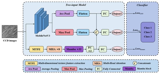
Figure 1. The overall dual-branch architecture of the proposed MTFE-Net model.

The dual-path design fuses the deep learning information and texture feature information, which ensures the balance between interpretability, model adaptability and computational efficiency at the structural level, and effectively improves the classification accuracy. The MTFE module (Figure 2) extracts the texture information of the image. This information is processed by the MHA mechanism and the Mamba algorithm, and then fused with the data processed by the pattern recognition deep neural network. The fused tensor can simultaneously represent the texture features of the roughness image and the information of the image itself.

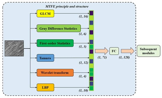
Figure 2. Schematic diagram of the MTFE module.

2.2. Multi-Dimensional Texture Feature Extraction

2.2.1. Global Statistics

The designed MTFE method integrates GLCM, gray-level difference statistic, first-order statistic, and Tamura texture features. These methods aim to describe the global texture feature statistics. The computational results of these algorithms also encode the images to be processed from their respective unique perspectives.

GLCM calculates the frequency of pixel pairs that are at a fixed distance (d) and in a specific direction (θ) within the image. The co-occurrence matrix characterizes the probability of two-pixel gray levels occurring simultaneously. It is defined by the joint probability density of the pixels at two positions. The result reflects the distribution characteristics of pixels with the same brightness and those with similar brightness, and it represents the brightness variation characteristics of an image in a certain direction. Let f (x, y) be a two-dimensional digital image with size M × N and gray level $N_g$ and suppose the distance between points $\left(x_1,y_1\right)$ and $\left(x_2,y_2\right)$ is d, and the angle between them and the horizontal axis is θ, then the GLCM that satisfies certain spatial relationships is as follows:

$$P\left(i,j,d,\mathrm{\theta }\right)=\#\left\{\left(x_1,y_1\right),\left(x_2,y_2\right)\in M\times N|f\left(x_1,y_1\right)=i,f\left(x_2,y_2\right)=j\right\}$$

(1)

Here, “#” represents the number of elements in the set. The grayscale value of the pixel point $\left(x_1,y_1\right)$ is i, and the grayscale value of the pixel point $\left(x_2,y_2\right)$ is j. Clearly, P is a matrix of size $N_g$ × $N_g$, and thus various gray-level co-occurrence matrices of different spacings and angles can be obtained from P. In this article, the azimuth angles are set at 0°, 90°, 45°, 135°, and the distance is set at 1. For the textures of different pixel gray values, the concentration of matrix elements can characterize the differences in the textures. Among the statistical quantities derived from GLCM, 16 statistical quantities including contrast (CON), inverse difference moment (IDM), energy (ASM), and correlation (COR) in four different directions were selected. Their formulas are as follows:

$$CON={{\displaystyle {\sum }_i{\displaystyle {\sum }_j\left(i-j\right)}}}^{2}P\left(i,j,d,\mathrm{\theta }\right)$$

(2)

$$IDM={\displaystyle {\sum }_i{\displaystyle {\sum }_j\frac{P\left(i,j,d,\mathrm{\theta }\right)}{1+|i-j|}}}$$

(3)

$$ASM={\displaystyle {\sum }_i{\displaystyle {\sum }_j{P}^2\left(i,j,d,\mathrm{\theta }\right)}}$$

(4)

$$COR={\displaystyle \frac{{\displaystyle {\sum }_i{\displaystyle {\sum }_j\left(i-{\mathrm{\mu }}_x\right)\left(j-{\mathrm{\mu }}_y\right)}}P\left(i,j,d,\mathrm{\theta }\right)}{{\mathrm{\sigma }}_x{\mathrm{\sigma }}_y}}$$

(5)

CON represents the texture clarity. The larger the value, the more intense the local gray level variation. IDM characterizes local homogeneity. The larger the value, the smoother the texture. ASM characterizes the uniformity of texture. The larger the value, the more regular the gray-scale distribution. COR represents the linear correlation of gray levels, and a larger value indicates directional textures.

The gray-level difference statistical method is a texture feature extraction approach based on the local gray difference of images. It describes the roughness, contrast, regularity, etc. of textures by analyzing the statistical characteristics of the gray changes in adjacent pixels. Let the image be f (x, y), and the gray-level difference between the point (x, y) and the offset point (x + Δx, y + Δy) is as follows:

$$g_{\mathrm{\Delta }}\left(x,y\right)=f\left(x,y\right)-f\left(x+\mathrm{\Delta }x,y+\mathrm{\Delta }y\right)$$

(6)

Here, Δx and Δy represent small displacements which are taken as 1 pixel, and $g_{\mathrm{\Delta }}$ is referred to as the gray-level difference. Select the horizontal, vertical and diagonal directions as the directions for calculating the gray-level difference. From $g_{\mathrm{\Delta }}$ as the gray-level difference, obtain the probability distribution $p_{\mathrm{\Delta }}\left(k\right)$ of the gray-level difference. The range of k is the same as the range of gray-level difference, which is [−m, m]. This distribution reflects the local variation intensity of the texture: if $p_{\mathrm{\Delta }}\left(k\right)$ has a higher probability at smaller values of k, it indicates that the texture is rough; if the distribution is flat, then the texture is fine. The mean (MEAN) and angular second moment (ASM) of the distribution are selected to encode the image. The calculation formula is as follows:

$$MEAN={\displaystyle \frac{1}{m}}{\displaystyle \sum _{k=-m}^m\left|k\right|\cdot p_{\mathrm{\Delta }}\left(k\right)}$$

(7)

$$ASM={\displaystyle \sum _{k=-m}^m{\left[p_{\mathrm{\Delta }}\left(k\right)\right]}^2}$$

(8)

The physical meaning of MEAN is overall roughness. A larger value indicates a rough texture and a smaller value indicates a fine texture. ASM describes the uniformity of the texture. A higher value indicates that the gray-level differences are concentratedly distributed and a lower value indicates a more dispersed distribution. The gray-level difference statistic method involves six statistical quantities in the encoding process.

The texture feature of first-order statistic is a statistical analysis method based on the image gray-level histogram. Different from GLCM and gray-level difference statistic, its core idea is to describe the macroscopic properties of texture by quantifying the distribution pattern of pixel gray values in the image, ignoring the spatial positional relationship between pixels. Let the range of image gray levels be [0, L − 1], where L represents the maximum gray level. The gray histogram H(k) indicates the frequency of occurrence of gray value k. The probability distribution of gray levels is as follows:

$$p\left(k\right)={\displaystyle \frac{H\left(k\right)}{N}},k=0,1,\dots ,L-1$$

(9)

Here, N represents the total number of pixels in the image. The histogram reflects the overall gray-level distribution of the image. Select the mean, variance and standard deviation of p(k) to characterize the overall gray-scale distribution of the image. The mean value describes the overall brightness level of the image. A high mean value corresponds to bright textures, while a low mean value corresponds to dark textures. The mean and standard deviation measure the degree of dispersion of the gray-level distribution. A larger mean indicates a higher contrast and sharper edges, while a smaller mean suggests a more uniform gray level. Therefore, the first-order statistic introduced three parameters for quantifying the image.

Tamura texture feature is a texture description method based on human visual perception, proposed by Tamura et al. in 1978 [36]. Its core idea is to quantify the six perceptual attributes of texture by a mathematical model: coarseness, contrast, directionality, line likeness, regularity and roughness. The coarseness, contrast and directionality were selected as the statistical quantities for quantifying the image. A total of 32 parameters are involved in characterizing the target image. The coarseness describes the granularity of the texture, reflecting the size of the basic units of the texture and their repetition frequency. The larger the elementary size or the lower the repetition rate, the rougher the texture. The contrast measures the dynamic range of gray levels and the degree of polarization, and is influenced by edge sharpness and the shape of the histogram. The directionality quantifies the consistency of the texture direction. For example, a high degree of stripe texture directionality indicates a high degree of consistency, while a low degree of random texture directionality indicates a low degree of consistency. The Tamura texture feature converts visual perception into statistical models such as histograms, gradient moments, and multi-scale averages, which simulate the sensitivity of the human eye to texture structures. The advantage of this algorithm is that the physical meaning of the features is clear and it conforms to cognitive intuition. Due to the complexity of the calculation, the global gray mean of the gray-scale image is used to approximate the coarseness, the global gray standard deviation of the gray-scale image is used to approximate the contrast, and the gradient direction gray distribution histogram data is used to approximate the directionality data.

In the surface roughness identification task, the four algorithms including GLCM, gray-level difference statistic, first-order statistic and Tamura texture features can significantly improve the detection accuracy, robustness and applicability. In the analysis of global feature quantities, the method combining multiple texture features and the method of jointly modeling spatial structure and statistical characteristics can complement each other and enhance the recognition accuracy.

GLCM captures the directional and local structure of texture through the statistical quantities of pixel pairs, and is sensitive to the depth of microscopic surface grooves. The gray-level difference statistic focuses on the variation of gray levels and quantifies the roughness, which is suitable for describing the subtle textures that are randomly distributed. First-order statistic is extracted from the global histogram to reflect the overall gray-level distribution pattern, which indicates the macroscopic uniformity. Tamura combined multi-scale statistical methods to simulate the human eye’s perception of the basic element size, which is more in line with subjective roughness evaluation. After integrating these four algorithms, MTFE can comprehensively represent the macroscopic and global texture properties, avoiding the bias of a single algorithm towards a specific texture type.

2.2.2. Frequency Domain Statistical Features and Local Statistical Features

Wavelet transform texture feature extraction is an image processing method based on multi-scale analysis. By decomposing the frequency components of the image in different scales and directions, it quantifies the structural characteristics of the texture. This algorithm generates wavelet basis functions by using the translation and scaling of the mother wavelet, and simultaneously captures both time-domain and frequency-domain information during the transformation. Perform two-dimensional discrete wavelet transform image decomposition using discrete wavelet transform. Using multi-resolution analysis (MRA), the signal is decomposed iteratively through the low-pass filter h[n] and the high-pass filter g[n]:

$$\begin{array}{l}{c}_{j+1}\left[k\right]={\displaystyle \sum _{n}h\left[n-2k\right]c_j\left[n\right]}\\ d_{j+1}\left[k\right]={\displaystyle \sum _{n}g\left[n-2k\right]c_j\left[n\right]}\end{array}$$

(10)

Here, c_j represents the coefficient of the j-th layer, d represents the detail component and the amount of data after decomposition is halved. This algorithm employs dual-orthogonal wavelets as the mother wavelets. The biorthogonal wavelets have balanced time-frequency localization capabilities, making them suitable for analyzing non-stationary surface textures. To save computing resources, this algorithm employs two different-scale frequency sub-bands, including a low-frequency distribution and a high-frequency detail distribution. The low-frequency distribution retains the overall outline of the image and reflects the macroscopic structure, while the high-frequency detail distribution captures the microscopic texture details. This algorithm uses mean and standard deviation statistics to compress the information of the low-frequency distribution and the high-frequency detail distribution. Wavelet transform decomposes the texture into a linear combination of scale-space orthogonal bases, and quantifies the multi-resolution texture structure through coefficient statistics. Wavelet transform, through multi-scale time-frequency analysis, can simultaneously capture both local details and global structure, and can analyze textures ranging from macroscopic outlines to microscopic details.

LBP is a texture feature description operator based on local gray-level differences. Its core idea is to generate codes by binarizing the gray-level differences between the neighboring pixels and the central pixel, to describe the local texture structure. Neighborhood binarization is the fundamental mathematical principle of LBP. Within a 3 × 3 window, the gray value of the central pixel $I_c$ is used as the threshold. The gray values of its eight adjacent pixels $I_p$ (p = 0, 1, …, 7) are compared, and an eight-bit binary code is generated. The formula is as follows:

$$LBP={\displaystyle \sum _{p=0}^{7}s\left(I_p-I_c\right)\cdot 2^p},s(x)=\left\{\begin{array}{l}1,x\ge 0\\ 0,x<0\end{array}\right.$$

(11)

The feature extraction method utilizes the statistical histogram to divide the image into sub-regions, calculates the LBP value histogram for each region, and concatenates all the sub-histograms to form a global feature vector:

$$H(k)={\displaystyle \sum _{i,j}\mathrm{\delta }\left(LBP(i,j)-k\right)},\mathrm{\delta }(x)=\left\{\begin{array}{l}1,x=0\\ 0,otherwise\end{array}\right.,k\in \left[0,B-1\right]$$

(12)

Among them, the number of histogram bins B is set to 10, which means that a 10-dimensional vector will be output, suitable for the input of CNN. The LBP algorithm abstracts local textures into binary encoding based on gray-level differences. By quantifying the global distribution through statistical histograms, it has the advantages of low computational complexity, strong robustness, and strong adaptability to posture.

Wavelet transform focuses on multi-scale and directional frequency domain enhancement, decomposing the image into different frequency sub-bands. Among them, the high-frequency sub-bands can suppress noise interference and improve feature stability. LBP focuses on local structure enhancement and invariance, encoding local gray-scale differences and being sensitive to surface micro-irregularities. The uniform LBP mode further reduces the dimensionality, improving computational efficiency. LBP has rotation and illumination invariance, and can retain the spatial locality of texture, avoiding the loss of position information in global statistics. These two algorithms effectively make up for the shortcomings of global statistics in their insensitivity to microscopic local textures. The incorporation of wavelet transform algorithm and LBP algorithm essentially involves introducing frequency domain analysis and local structure description, thereby overcoming the limitations of traditional texture features, which are characterized by a single scale and sensitivity to noise.

MTFE concatenates six texture statistical features through the concat method. Its concatenation process can be mathematically expressed as follows:

$$F_{MTFE-cat}=\left[F_{GLCM};F_{GDS};F_{FOS};F_T;F_{WT};F_{LBP}\right]$$

(13)

Among them, $F_{MTFE-cat}\in {ℝ}^{B\times W_{MTFE}}$ represents the result of the concat method of MTFE, $F_{GLCM}\in {ℝ}^{B\times W_1}$ represents the result of the GLCM algorithm, $F_{GDS}\in {ℝ}^{B\times W_2}$ represents the result of the gray difference algorithm, $F_{FOS}\in {ℝ}^{B\times W_3}$ represents the result of the first-order statistic, $F_T\in {ℝ}^{B\times W_4}$ represents the Tamura texture feature result, $F_{WT}\in {ℝ}^{B\times W_5}$ represents the wavelet transform result, and $F_{LBP}\in {ℝ}^{B\times W_6}$ represents the LBP algorithm result. $W_1$, $W_2$, $W_3$, $W_4$, $W_5$ and $W_6$ represent the number of output results of this algorithm. $W_{MTFE-cat}$ is the sum of $W_1$, $W_2$, $W_3$, $W_4$, $W_5$ and $W_6$. After concatenation, the result is transformed into a 128-length texture feature tensor through the FC layer.

MTFE has implemented a multi-dimensional feature complementation mechanism. It achieves a complementary scale between the macroscopic outline and the microscopic structure. All algorithms jointly describe the overall morphology and jointly capture the local irregularity. It achieves a spatial relationship complementarity between structural statistics and local patterns, covering texture types ranging from regular to disordered. It achieves a statistical characteristic complementarity between global distribution and local dynamics balance. The overall gray-scale distribution description, multi-scale characteristics, and frequency domain characteristics jointly solve the contradiction between uniformity and local mutations. The essence of this algorithm is to construct a collaborative description system with multiple scales, multiple dimensions and multiple statistics, thereby achieving comprehensive scale coverage, complete spatial description, balanced statistical representation, and efficient engineering implementation.

2.3. Multi-Dimensional Texture Feature Processing

MHA Mechanism

The MHA mechanism enhances the model’s ability to capture complex relationships by performing parallel computations of multiple attention heads. The mathematical framework of the MHA mechanism originates from the self-attention architecture. Its specific structure includes input and linear transformation, head splitting, scaled dot-Product attention, and multi-head output integration.

The embedding representation of the given sequence is $X\in {ℝ}^{n\times d}$, where n is the sequence length and d is the feature dimension. There are h attention heads in total. For each attention head i, an independent learnable parameter matrix is used to generate the query, key, and value vectors:

$$Q_i=X{W}_i^Q,K_i=X{W}_i^K,V_i=X{W}_i^V$$

(14)

Here, $W_i^Q,W_i^K\in {ℝ}^{d\times d_k}$, $W_i^V\in {ℝ}^{d\times d_v}$, and $d_k=d_v={\displaystyle \frac{d}{h}}$. In head splitting, split Q, K, and V along the feature dimension into h independent subspaces:

$$hea{d}_i=Attention\left(Q_i,K_i,V_i\right)$$

(15)

The dimension of each head is reduced to $d_i$, thereby reducing the computational load and enabling parallelization. In scaled dot-Product attention, for each head, the dot product of the query and the key is calculated, and it is scaled to prevent gradient instability:

$$Attention\left(Q_i,K_i,V_i\right)=\mathrm{softmax}\left({\displaystyle \frac{Q_i{K}_i^T}{\sqrt{d_k}}}\right)V_i$$

(16)

Here, softmax normalization converts the dot product result into a probability distribution, representing the attention weights at different positions. Finally, concatenate the outputs of h heads along the feature dimension, and the dimension is restored to n × d after concatenation. By mapping through a learnable matrix to the target space, the final output becomes consistent with the input dimension.

The MHA mechanism possesses the characteristic of multi-perspective modeling, and can generate feature representations for different subspaces. This also enables the algorithm to have the ability to capture diverse relationships such as semantics and positions. Long-distance dependency optimization is also an advantage of this algorithm. It solves the problem of vanishing gradients and enables it to have parallel computing capabilities, significantly improving the training speed. The scaled dot-Product ensures that the distribution is stable before the input reaches the softmax function, preventing the occurrence of gradient explosion or vanishing. The limitation of the MHA mechanism is that the complexity of pointwise multiplication is not favorable for long sequences, and it needs to be optimized. It has also been noted that the MHA mechanism also has the defect of having a local receptive field.

Regarding the issue of local receptive field, this algorithm introduces the Mamba model which has a global receptive field. Mamba is a sequence processing architecture based on the selective state space model. Through dynamic parameter adjustment and hardware optimization, it achieves linear computational complexity and efficient modeling of long sequences. The core of its mathematical principle lies in the combination of the discretization of the state space model, the selective mechanism, and the hardware-aware algorithm. The core of Mamba is the continuous-time state space model, which describes the system dynamics through differential equations:

$$\begin{array}{l}{h}^{\prime }(t)=\mathbf{A}h(t)+\mathbf{B}x(t),\\ y(t)=\mathbf{C}h(t)+\mathbf{D}x(t),\end{array}$$

(17)

Here, A $\in {ℝ}^{n\times n}$, B $\in {ℝ}^{n\times 1}$, C $\in {ℝ}^{1\times n}$, D $\in {ℝ}^1$ are the weighting parameters, x(t) represents the input of the texture feature sequence, y(t) represents the output of the texture feature sequence, and h(t) represents the hidden state. The model employs Zero-Order Hold (ZOH) to discretize the continuous system, thereby converting the model into a sequence-to-sequence mapping. Mamba’s breakthrough lies in the introduction of a selective mechanism, namely the selective scanning algorithm. It utilizes the associativity law to decompose the sequence into sub-blocks for parallel computation, and then combines the results. Hardware perception optimization combines the discretization, scanning, and output projection into a single GPU core, reducing the number of memory accesses. The linear complexity of Mamba is significantly superior to the quadratic growth of the Transformer. Recursive structure supports streaming generation and is suitable for texture feature sequence tasks. Therefore, Mamba’s innovation lies in the intelligent information filtering capability bestowed by its selective mechanism, enabling it to outperform Transformer in terms of efficiency and expression ability, and thus becoming a new paradigm for long sequence modeling.

The combination of Mamba and MHA achieves a significant breakthrough in long sequence processing, computational efficiency, and representational capability by complementing the core advantages of both. This combination achieves a balance between linear complexity and global modeling. Mamba possesses a linear complexity advantage, which overcomes the global modeling bottleneck of the attention mechanism. This combination has further achieved dynamic selectivity and enhanced spatial perception. The dynamic information filtering capability of Mamba, combined with the spatial interaction ability of the attention mechanism, has achieved state updates based on content perception, and directly established the relationships among any texture features. The combination of these two algorithms demonstrates the synergy between local details and global semantics.

2.4. Combination of Neural Network Coding and Texture Feature Coding

This algorithm (as shown in Figure 3) employs a dual-encoding fusion strategy that combines neural network encodings of roughness images with texture feature encodings to execute pattern recognition tasks. By strategically concatenating these complementary representations, the algorithm maximizes retention of intrinsic data information, enables effective downsampling for pattern extraction, and enriches complex texture–feature relationships—significantly boosting model robustness in roughness-sensitive applications.

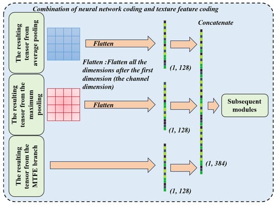
Figure 3. A schematic diagram of the combination of neural network coding and texture feature coding.

The traditional encoding method has many limitations. Roughness images depict surface irregularities quantified by metrics like Tamura roughness or fractal dimension. Isolated neural encoders often fail to capture multi-scale texture patterns. Texture features lack contextual semantics for high-level pattern abstraction. Independent processing loses critical interactions between topological structures and statistical texture properties. Fusion via concatenation bridges these gaps by creating a unified, information-dense representation before downsampling operations. This preserves discriminative attributes often lost in serialized processing pipelines.

The algorithm implements two fusion strategies, each with distinct structural and computational properties. Its detailed mathematical representation is as follows:

$$F_{cat}=\left[F_N;F_T\right]=\left[\underset{Neural Features}{\underbrace{f_1 , \dots , f_n}};\underset{Texture Features}{\underbrace{f_1 , \dots , f_t}}\right]$$

(18)

Here, $F_{cat}\in {ℝ}^{B\times W}$ represents the combined tensor, $F_N\in {ℝ}^{B\times W_1}$ represents the neural encoder outputs, and $F_T\in {ℝ}^{B\times W_2}$ represents the texture encoder outputs. $W_1$ is 256, $W_2$ is 128, and $W$ is the sum of $W_1$ and $W_2$. B represents the batch size set during the model training process.

This algorithm endows the overall model with advantages over traditional methods. The algorithm possesses spatial alignment integrity. Per-pixel alignment preserves local texture–structure correlations that are critical. The combination of the two encoding methods exhibits multi-scale robustness. The neural encoder captures hierarchical abstract features ranging from edges to shapes to objects but loses fine texture details during the pooling operation. The texture encoder quantifies statistical patterns but ignores spatial semantics. Complementary channels resolve ambiguities. Neural activations detect macro-structures while MTFE refines micro-textures.

Concatenating neural and texture encodings creates a synergistic representation that overcomes the limitations of isolated approaches. By preserving spatial–textural interactions during downsampling, this fusion strategy significantly enhances robustness, accuracy, and efficiency in roughness-centric pattern recognition. Channel-wise and sequence concatenation offer complementary advantages.

2.5. Loss Function Design

This algorithm employs three output modes, namely the output from the neural network, the output of the texture features, and the combined output of the neural network and the texture features. Therefore, there are three loss functions involved. All three methods employ cross-entropy loss during the operation:

$$L=-{\displaystyle \sum _{c=1}^C{y}_c\log \left({\widehat{y}}_c\right)}$$

(19)

Here, the true label is the one-hot vector $\left[y_1,\dots ,y_c\right]$ and the prediction probability is $\left[{\widehat{y}}_1,\dots ,{\widehat{y}}_c\right]$. The cross-entropy loss has a large gradient when there is an incorrect prediction, and it converges quickly, making it a commonly used function in classification tasks. Its synergy with softmax and sigmoid enables efficient gradient calculation, and compared to other loss functions, it is more suitable for the probabilistic nature of classification tasks.

3. Experiment

3.1. Experimental Process

The process of the experiment is shown in Figure 4. The entire process of the experiment includes dataset construction, dataset building, model construction, and model training.

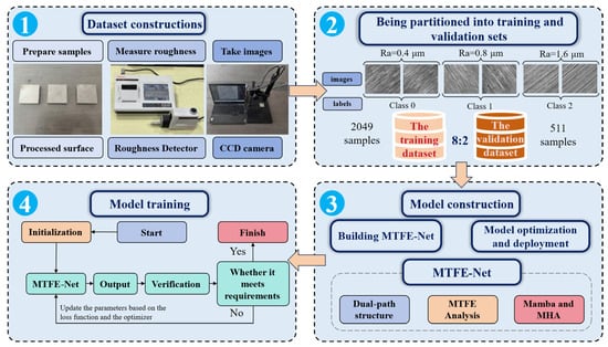
Figure 4. The experimental and data processing workflow, outlining the key stages from sample preparation and image acquisition (element 1), dataset splitting (element 2), model construction (element 3) and model training (element 4).

3.2. Dataset Constructions and Dataset Building

Dataset constructions are shown in Figure 4 (element 1). In this study, Q235 steel (Figure 5a) was selected as the workpiece material and machined under varying parameters. Use 46-grade sandpaper to grind out a class 0 surface, obtaining a plane with Ra less than 0.4 μm (considering the surface Ra as 0.4 μm). Use 100-grade sandpaper to grind out a class 1 surface, obtaining a plane with an Ra value between 0.4 μm and 0.8 μm (considering the surface Ra as 0.8 μm). Then, through the wire drawing process, manufacture a class 2 surface, obtaining a plane with an Ra value between 0.8 μm and 1.6 μm (considering the surface Ra as 1.6 μm). Take class 2 as an example. The morphological difference between a surface with a roughness of 0.8 μm and a slightly rougher surface with a roughness of 1.6 μm is not obvious, and this difference is mainly determined by fine structural features that are difficult to clearly distinguish. The same applies to the other groups. Therefore, we classify it as belonging to the same category of roughness. Surface roughness measurements were obtained at 16 distinct locations per sample using a Mitutoyo SJ-410 (Figure 5b) contact-based surface profilometer, with the mean value representing overall roughness. The measurement range of the equipment is set at 8 μm, and the resolution at this range is 0.0001 μm.

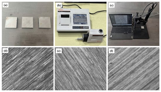
Figure 5. Visual examples of surface images for the three roughness classes of Q235 steel under natural lighting conditions. (a) The Q235 steel samples. (b) Mitutoyo SJ-410 contact-based surface profilometer. (c) The CCD camera and the shooting system. (d) Class 0 (Ra = 0.4 μm); (e) Class 1 (Ra = 0.8 μm); (f) Class 2 (Ra = 1.6 μm).

Dataset building is shown in Figure 4 (element 2). To build the dataset, samples were mounted on an optical platform. The experimental process requires exposure to natural light. Specifically, the setup utilized a fixed-position, diffuse natural daylight source to illuminate the sample surfaces. The angle of incidence was set to about 45°, a standard in metallographic analysis, to provide a balanced contrast of surface topography while minimizing specular reflections that can obscure texture details. When imaging under natural light, the laser source should be turned off to eliminate spectral interference, enabling the capture of textures under environmental conditions. A fixed industrial camera (Figure 5c) captured images under natural light at identical sample positions, generating 2560 geometrically registered images. The 2560 pictures consist of 880 pictures of Class 0, 720 pictures of Class 1, and 960 pictures of Class 2. The surface roughness of these samples is classified into three grades: Class 0 (Figure 5d), Class 1 (Figure 5e), and Class 2 (Figure 5f). The dataset was partitioned into training and validation sets at an 8:2 ratio, comprising 2049 and 511 samples, respectively. This 8:2 ratio was chosen to provide a substantial amount of data for the model to learn the complex, multi-scale texture features effectively, while still retaining a sufficiently large and representative independent validation set to ensure a reliable and unbiased evaluation of the model’s generalizability and to mitigate the risk of overfitting. Figure 5 illustrates surface images of workpieces processed with different parameters under natural light.

3.3. Model Construction and Model Training

Model construction is shown in Figure 4 (element 3). After the dataset is constructed, the MTFE-Net model is built and the parameters of the model are initialized. The training set and validation set of the dataset are used to train the model and adjust its parameters until the model meets the requirements.

Model training is shown in Figure 4 (element 4). In the experiment, all models were implemented using the PyTorch (2.0.1) framework on a single NVIDIA GTX 3090 graphics processor. To achieve rapid convergence, the stochastic gradient descent (SGD) optimizer was employed to train all models. The learning rate was adjusted dynamically.

3.4. Evaluation Metrics

The accuracy, precision, recall, and F1-score are selected as the final evaluation criterion. The collaborative analysis of these four indicators can comprehensively assess the performance of the model in terms of accuracy, precision, recall, and F1-score, avoiding the one-sidedness of a single indicator.

Accuracy refers to the proportion of samples that are predicted correctly by the model out of the total sample:

$$Accuracy={\displaystyle \frac{TP+TN}{TP+TN+FP+FN}}$$

(20)

Here, True Positive (TP) is defined as the case where the actual class is positive and the prediction is also positive; True Negative (TN) is defined as the case where the actual class is negative and the prediction is negative; False Positive (FP) is defined as the case where the actual class is negative but is predicted as positive, which is a false alarm; False Negative (FN) is defined as the case where the actual class is positive but is predicted as negative, which is a missed detection.

Precision is defined as the proportion of samples predicted by the model to be of the positive class, among which the actual class is also positive.

$$Precision={\displaystyle \frac{TP}{TP+FP}}$$

(21)

Recall refers to the proportion of actual positive samples that are correctly identified by the model.

$$Recall={\displaystyle \frac{TP}{TP+FN}}$$

(22)

F1-score is the harmonic mean of precision and recall, comprehensively balancing the performance of both.

$$F1=2\times {\displaystyle \frac{Precision\times Recall}{Precision+Recall}}$$

(23)

4. Results and Discussion

4.1. Interpretation of Ablation Studies and Model Efficacy

To evaluate the incremental contribution of each major component in the MTFE-Net architecture, a series of ablation experiments were designed. This involved progressively building the model from a baseline neural network branch (Mobile-Net) and sequentially integrating the MTFE module, the MHA mechanism, and the Mamba model.

The progressive improvement in performance metrics across the ablation studies (as shown in Table 1) validates the hierarchical contribution of each component. The baseline model, relying solely on the neural network branch, already achieves a respectable accuracy of 93.02%. This confirms that deep learning models can indeed learn meaningful representations related to surface roughness from image data alone. However, the significant jump in accuracy to 94.64% upon integrating the MTFE branch underscores the critical limitation of pure deep learning approaches: their tendency to overlook handcrafted, physically interpretable features that are highly relevant to the task. The MTFE module compensates for this by providing a rich, multi-dimensional descriptor, which are directly correlated with surface topography.

Table 1. Ablation study of each component.

Method	MTFE	MHA	Mamba	Accuracy	Precision	Recall	F1-Score
MTFE-Net				0.9302	0.9266	0.9210	0.9227
	√ 1			0.9464	0.9422	0.9408	0.9411
	√	√		0.9490	0.9450	0.9429	0.9437
	√		√	0.9477	0.9464	0.9396	0.9418
	√	√	√	0.9523	0.9489	0.9467	0.9474

¹ “√” indicates that this experimental model has this module, and the same applies below.

The subsequent incorporation of MHA and Mamba further refines the model’s performance. The individual addition of either MHA or Mamba led to improvements, but the highest performance was achieved when both were used together. This synergy can be explained by their complementary strengths. The MHA mechanism excels at capturing complex, long-range dependencies within the sequence of texture features, effectively identifying and weighting the most discriminative elements from the MTFE output. However, its computational complexity and potential limitations with local receptive fields are well-known. The Mamba model, with its selective state space mechanism and linear computational complexity, introduces a global receptive field and a dynamic filtering capability, allowing it to focus on or ignore specific parts of the feature sequence based on the input content. The combination effectively creates a powerful feature processing pipeline where MHA highlights key inter-feature relationships and Mamba efficiently models their sequential dynamics, leading to a more robust and nuanced representation.

4.2. The Critical Role of Multi-Dimensional Feature Complementarity

A second ablation study was performed to deconstruct the MTFE module itself, testing the individual and combined contributions of its constituent algorithms: global statistics, LBP, and wavelet transform.

The components of the MTFE module (as shown in Table 2) offer profound insights. The results clearly show that relying on a single category of features—be it global statistics, LBP, or wavelet transform—yields suboptimal performance. For instance, using only wavelet transform features resulted in the lowest accuracy of 87.78%, suggesting that frequency-domain information alone is insufficient for this task. This is logical, as surface roughness is a complex phenomenon manifested in both spatial and frequency domains.

Table 2. Ablation study of each part of MTFE module.

Method	Global Statistics	LBP	Wavelet Transform	Accuracy	Precision	Recall	F1-Score
MTFE-Net	√ 1			0.9451	0.9447	0.9363	0.9388
		√		0.9033	0.9032	0.8880	0.8899
			√	0.8778	0.8672	0.8640	0.8647
	√	√		0.9458	0.9417	0.9395	0.9400
	√	√	√	0.9523	0.9489	0.9467	0.9474

¹ “√” indicates that this experimental model has this module, and the same applies below.

The true power of the MTFE module is revealed in the incremental performance gain as features are combined. The combination of global statistics and LBP already outperforms the baseline, and the full integration of all three categories achieves the peak performance. This validates the paper’s core thesis of “multi-dimensional feature complementarity.” The global statistics provide a macroscopic overview of the image’s texture. The LBP operator captures fine-grained, local micro-structures and offers invariance to illumination changes. Wavelet transform bridges the gap by offering a multi-scale analysis that captures both macroscopic outlines and microscopic details in the frequency domain. Together, they form a comprehensive description system that is far more resilient and informative than any single approach.

4.3. Model Selection

To optimize the model’s configuration, hyperparameter sensitivity analyses were conducted for both the MHA and Mamba components (as shown in Table 3 and Table 4), testing their performance with different numbers of layers to identify the optimal settings of eight heads for MHA and 32 layers for Mamba.

Table 3. Comparison of MHA with different number of layers in MTFE-Net.

Method	Number of Layers	Accuracy	Precision	Recall	F1-Score
MTFE-Net	4	0.9451	0.9423	0.9380	0.9393
	8	0.9523	0.9489	0.9467	0.9474
	16	0.9451	0.9417	0.9381	0.9393

Table 4. Comparison of Mamba with different number of layers in MTFE-Net.

Method	Number of Layers	Accuracy	Precision	Recall	F1-Score
MTFE-Net	4	0.9444	0.9397	0.9387	0.9388
	8	0.9471	0.9456	0.9390	0.9410
	16	0.9431	0.9419	0.9344	0.9367
	32	0.9523	0.9489	0.9467	0.9474
	64	0.9412	0.9369	0.9344	0.9352

The experiments varying the number of layers for MHA and Mamba provide practical guidance for model configuration. For MHA, the eight-head configuration proved optimal. Fewer heads may lack sufficient representational capacity to model diverse feature relationships, while more heads could introduce redundancy or overfitting, leading to a slight drop in performance. For Mamba, the 32-layer configuration was best, indicating that a certain depth is necessary to model the complex state transitions of the texture feature sequence effectively.

4.4. Different Encoders

The selection of the encoder in the neural network branch is critical, as it determines the quality of the automatically learned features that will complement the handcrafted MTFE features. Table 5 evaluates the impact of various mainstream encoders on the overall performance of MTFE-Net. As detailed in the accompanying table, we benchmarked a range of models, including ResNet family variants, VGG16, Swin Transformer, VMamba, and Mobile-Net.

Table 5. Ablation studies of different encoders.

Method	Encoder	Complexity (G)	Parameters (M)	Accuracy	Precision	Recall	F1-Score
MTFE-Net	ResNet18 [37]	9.72	12.37	0.8392	0.8315	0.8323	0.8301
	ResNet34 [37]	19.41	22.48	0.8235	0.8125	0.8138	0.8117
	ResNet50 [37]	22.35	26.91	0.8216	0.8054	0.8017	0.8025
	ResNet101 [37]	41.85	45.90	0.8235	0.8132	0.8029	0.8044
	VGG16 [37]	80.94	15.91	0.7863	0.7839	0.7614	0.7606
	Swin Transformer [33]	15.23	67.12	0.8137	0.8134	0.7861	0.7853
	VMamba [35]	31.35	33.98	0.3922	0.1307	0.3333	0.1878
	Mobile-Net	1.18	3.28	0.9523	0.9489	0.9467	0.9474

The results reveal a clear and significant trend: heavier and more complex encoders, such as ResNet101, yielded poor performance, respectively. In stark contrast, the lightweight Mobile-Net encoder achieved the highest accuracy of 95.23% while maintaining minimal computational cost. This superior performance underscores a key insight of our fusion strategy: the primary role of the neural network branch is not to single-handedly solve the problem, but to provide a complementary set of features to the rich, physically-grounded MTFE descriptors. Mobile-Net’s efficiency and ability to capture essential hierarchical features without overfitting make it the ideal partner. Its low complexity also ensures that the overall MTFE-Net model remains efficient and suitable for potential industrial deployment, where computational resources may be limited. Therefore, Mobile-Net was selected as the optimal encoder, perfectly aligning with the goal of creating a high-performance yet practical model.

4.5. Quantitative Comparison of Results with State-of-the-Art Models

To thoroughly evaluate the proposed method, MTFE-Net was benchmarked against a diverse set of state-of-the-art models, including vision transformers, advanced convolutional networks such as ResNeXt, Xception, and EfficientNet. The comparative results (as shown in Table 6) demonstrate the superior effectiveness.

Table 6. Quantitative comparison of results with state-of-the-art models. The best values in the column are in bold.

Method	Complexity (G)	Parameter (M)	FPS	Accuracy	Precision	Recall	F1-Score
Vision Transformers [38]	87.74	85.65	188.67	0.7373	0.7245	0.7166	0.7156
ResNeXt26ts [39]	9.61	8.22	220.85	0.8686	0.8559	0.8550	0.8554
ResNet18 [39]	9.53	11.18	344.82	0.8353	0.8309	0.8147	0.8164
Xception41 [39]	26.40	24.92	120.48	0.8294	0.8199	0.8053	0.8060
EfficientNet_b0 [39]	2.01	3.97	108.70	0.8333	0.8190	0.8155	0.8164
Res2Net50 [40]	22.10	23.01	60.98	0.8412	0.8394	0.8177	0.8189
MTFE-Net	1.18	3.28	34.48	0.9523	0.9489	0.9467	0.9474

MTFE-Net achieved a leading accuracy of 95.23%, significantly outperforming all competitors, with the next best model, ResNeXt26ts, trailing by over 8 percentage points. More importantly, this peak performance was accomplished with remarkably low computational complexity (1.18 GFLOPs) and a modest parameter count (3.28 M), making it substantially more efficient than other high-performing models. At the cost of sacrificing a certain amount of FPS, MTFE-Net achieved a significant improvement in accuracy. For instance, while Vision Transformers and Res2Net50 achieved accuracies below 85%, they required computational costs 74 and 18 times greater than MTFE-Net, respectively. This decisive advantage underscores the success of our core innovation: the synergistic fusion of handcrafted texture features and deep learning features.

4.6. Discussion

4.6.1. Confusion Matrix

To further elucidate the decision-making process of MTFE-Net and diagnose its limitations, we conducted a series of visualization analyses.

Based on the visual comparison of the four confusion matrices (Figure 6), the proposed MTFE-Net model demonstrates the most robust and balanced performance for surface roughness classification. Its matrix shows the highest and most concentrated correct classification rates along the diagonal, with errors almost exclusively occurring between adjacent classes. This indicates excellent discriminative power.

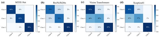
Figure 6. Confusion matrix for the models on the validation set. (a) MTFE-Net; (b) ResNeXt26ts; (c) Vision Transformers; (d) Xception41.

In contrast, the other models exhibit clear limitations. ResNeXt26ts shows more frequent misclassification. Vision Transformers display the weakest performance with lower diagonal values, suggesting it struggles with this task, likely due to data limitations. While Xception41 shows outstanding accuracy for Class 2, its performance on Classes 0 and 1 is comparatively weaker, indicating an imbalanced learning profile. This comparative analysis visually confirms that MTFE-Net’s hybrid feature fusion strategy yields superior generalizability across all roughness classes, avoiding the specific weaknesses observed in the other state-of-the-art models.

4.6.2. The Feature Response of the MTFE Module

The feature response of the MTFE module was quantified (Figure 7).

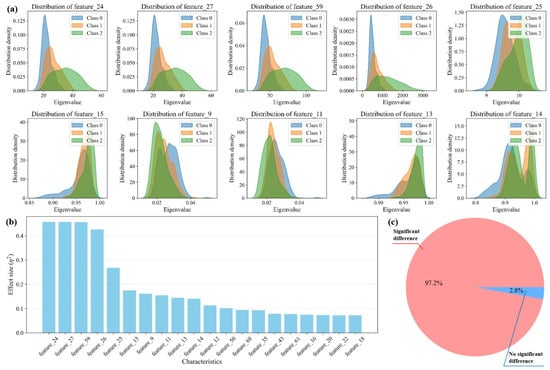
Figure 7. Visualization of the discriminative power of features extracted by the MTFE module. (a) Distribution density plots of ten selected texture features across the three roughness classes. (b) Bar chart of the effect sizes (η²) for all texture features. (c) Pie chart showing that 97.2% of the extracted features exhibit statistically significant differences between classes.

Based on the comprehensive analysis of the provided chart, the extracted texture features demonstrate remarkable richness and effectiveness in characterizing the image dataset. The three-panel visualization presents compelling evidence that these features capture substantial discriminative information across different image classes.

Figure 7a provides the most direct evidence of feature effectiveness through ten distribution density plots. Each subplot shows clear separation between the three classes across different texture features. The distinct distribution patterns indicate that these features capture fundamental differences in visual properties among classes. For instance, features like feature_24 and feature_27 show particularly well-separated density curves, suggesting they are highly effective at distinguishing between classes. The consistency of these separation patterns across multiple features indicates that the texture characteristics are capturing systematic variations rather than random noise. The overlapping areas between distributions are minimal in most cases, demonstrating that the features provide clean decision boundaries for classification tasks.

Figure 7b quantifies this discriminative power through effect size measurements (η²). The bar chart reveals that several features, particularly feature_24, feature_37, and feature_59, exhibit exceptionally high effect sizes, indicating strong capability to differentiate between classes. Effect sizes above 0.14 are generally considered large in statistical terms, and the presence of multiple features exceeding this threshold confirms that the texture features capture substantial between-class variance. The graduated effect sizes across different features suggest a complementary information structure where each feature contributes unique discriminative power, collectively forming a comprehensive descriptive framework.

The most convincing evidence comes from Figure 7c, where the pie chart shows that 97.2% of the extracted features demonstrate statistically significant differences between classes. This exceptionally high percentage is unusual in feature analysis and indicates that nearly all texture characteristics measured contain meaningful discriminative information. The minimal 2.8% of non-significant features suggests that the feature extraction process is highly efficient with minimal redundancy or noise.

The collective evidence from all three panels demonstrates that the texture features provide multi-faceted characterization of the image dataset. The distribution patterns in Figure 7a show how features capture class-specific characteristics, the effect sizes in Figure 7b quantify their relative importance, and the significance analysis in Figure 7c validates their statistical reliability. This multi-dimensional approach ensures that the features capture both macroscopic patterns through high-effect-size features and subtle variations through the comprehensive feature set. The consistency of results across multiple features indicates that the texture characteristics are robust descriptors that transcend specific image elements and capture fundamental visual properties. The features encode information about structural patterns, contrast variations, and spatial relationships that are class-specific and reproducible across the dataset.

4.6.3. The t-SNE Visualization

The t-SNE visualization comparing feature space separability is shown in Figure 8; MTFE-Net demonstrates superior discriminative capability. In Figure 8a, the data points for Class 0, 1, and 2 form the most compact and well-separated clusters, with minimal overlap. This indicates that its fused feature representation effectively distinguishes between different roughness levels.

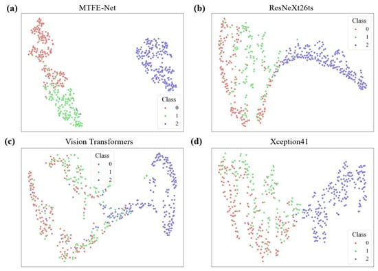
Figure 8. t-SNE visualization of the feature space for the results of models. (a) MTFE-Net; (b) ResNeXt26ts; (c) Vision Transformers; (d) Xception41.

In contrast, the other models show varying degrees of inferior separation. ResNeXt26ts (Figure 8b) and Xception41 (Figure 8d) display moderate clustering, but with more diffuse boundaries and greater inter-class mixing, particularly between Classes 1 and 2. Vision Transformers (Figure 8c) exhibits the poorest performance, with the three classes almost entirely overlapping into a single, indistinguishable cloud, suggesting its feature representation is poorly suited for this specific task. This visualization provides geometric proof for the quantitative results. The clear separation in MTFE-Net’s feature space directly explains its high classification accuracy, as distinct clusters are easily separable by a classifier. The confusion and overlap in the feature spaces of the other models visually justify their higher error rates, highlighting the unique effectiveness of MTFE-Net’s hybrid feature fusion approach.

4.6.4. The Heatmaps of MTFE-Net

The progressive feature evolution visualized through the heatmaps in Figure 9 provides compelling, interpretable evidence of how MTFE-Net distinguishes between surface roughness classes by learning representations that align with light scattering behavior. Each row corresponds to the processing trajectory for a specific class: (a) Class 0 (smoothest) shown in Figure 9a, (b) Class 1 (intermediate) shown in Figure 9b, and (c) Class 2 (roughest) shown in Figure 9c. The five heatmaps from left to right illustrate the feature refinement across key stages of the network of mobilenetV3.

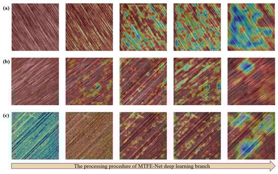
Figure 9. The heatmaps of the deep learning branch of MTFE-Net. The heatmaps from left to right are the process of deep learning. (a) Class 0; (b) Class 1; (c) Class 2.

For Class 0 surfaces, the initial heatmaps show a relatively diffuse and low-intensity activation pattern. As processing advances, the attention becomes moderately concentrated on subtle, fine-scale texture regions. This evolution is consistent with the scattering physics of smooth surfaces, where incident light undergoes primarily specular or low-angle scattering. The network learns to focus on faint, high-frequency texture variations—the primary visual cue distinguishing a very fine finish—while correctly ignoring non-existent strong, localized scatterers [11].

In contrast, the heatmaps for Class 2 surfaces exhibit a markedly different pattern. Strong, high-intensity activations emerge early, often highlighting distinct, isolated regions corresponding to pronounced peaks, valleys, or deep machining marks. These features act as strong, localized scattering centers under oblique illumination, generating significant contrast. The network’s progressive stages effectively amplify and integrate the signals from these dominant defects, constructing a representation dominated by these high-contrast, spatially discrete scatterers characteristic of rough surfaces.

The Class 1 heatmaps reveal an intermediate and highly informative state. The attention is more distributed than in Class 2 but shows greater structure and higher-intensity foci compared to Class 0. The network appears to capture a mix of moderate-frequency texture patterns and a few more prominent individual features. This aligns with the transitional scattering regime, where surface topography generates a broader distribution of scattering angles, resulting in a visual texture that combines both a granular background and occasional distinct scatterers.

This hierarchical attention progression demonstrates that MTFE-Net’s internal representations are physically grounded. The model learns to hierarchically identify and weigh the very surface morphological features that dictate optical scattering behavior. This validates that the proposed hybrid feature fusion enables a learning process that correlates with tangible surface physics, thereby offering a robust and interpretable framework for non-contact roughness assessment.

The final normalized heatmaps presented in Figure 10 offer a compelling visual dissection of the decision-making process within the proposed MTFE-Net, particularly highlighting the distinct and complementary roles of its dual-branch architecture. Each row corresponds to the feature refinement for a specific roughness class: (a) Class 0 (smoothest) shown in Figure 10a, (b) Class 1 (intermediate) shown in Figure 10b, and (c) Class 2 (roughest) shown in Figure 10c. A critical comparative analysis between the deep learning branch on the left and the MTFE module on the right halves of these heatmaps reveals a fundamental divergence in how surface features are perceived and prioritized, directly related to the identification of surface defects and machining traces.

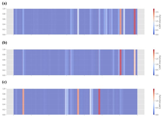
Figure 10. The final normalized heatmaps of MTFE-Net. (a) Class 0; (b) Class 1; (c) Class 2.

For the Class 0 surface (Figure 10a), the deep learning branch on the left exhibits a relatively uniform, low-intensity activation, suggesting it learns a generalized, holistic representation of a fine-textured, homogeneous surface. In stark contrast, the MTFE module on the right generates pronounced, localized activations. This indicates that the handcrafted texture features are acutely sensitive to subtle, residual micro-textures or faint directional patterns that remain even on a smooth finish. These features, potentially below the primary learning threshold of the deep network alone, are highlighted by the MTFE module as significant discriminative cues.

The heatmaps for the Class 2 surface (Figure 10c) demonstrate an inverse yet complementary relationship. Here, the deep learning branch shows strong, somewhat clustered activations, likely responding to the overall high-contrast, chaotic texture and gross topological variations characteristic of a rough surface. The MTFE module, however, provides a more structured and localized diagnosis. Its activations pinpoint specific, high-contrast linear streaks or isolated spots. This aligns perfectly with the physics of light scattering from rough surfaces, where distinct machining grooves, deep scratches, or isolated pits act as dominant, localized scatterers. The MTFE module effectively “zooms in” on these specific defect signatures, which are embedded within but not exclusively defined by the broader texture learned by the deep branch.

The Class 1 surface (Figure 10b) represents a transitional state. The activations from both branches are present and more balanced in intensity compared to the extreme classes. The deep learning branch begins to identify emerging texture complexity, while the MTFE module activates on a mixture of moderate-frequency patterns and a few nascent, more prominent features. This synergy suggests that for intermediate roughness, the model relies on a fusion of the deep branch’s understanding of the evolving global texture pattern and the MTFE branch’s detection of the specific, growing population of individual scattering sites.

In conclusion, the detailed analysis of MTFE-Net’s decision-making process, interpreted through the lens of scattering optics, reveals a physically grounded classification mechanism. The model’s dual-branch architecture synergistically combines the deep learning branch’s ability to capture holistic, global texture patterns with the MTFE module’s precision in identifying localized, defect-induced scatterers. For Class 0 surfaces, the heatmaps show diffuse activations focusing on subtle, high-frequency textures, consistent with the predominant specular or low-angle scattering from fine finishes. In contrast, Class 2 surfaces trigger strong, localized activations on distinct peaks, valleys, and machining marks, which act as dominant scattering centers under oblique illumination. The Class 1 heatmaps display a balanced response, capturing a mix of moderate-frequency patterns and emerging scatterers, aligning with a transitional scattering regime. This hierarchical attention progression, from faint textures to prominent defects, demonstrates that MTFE-Net’s feature representations are intrinsically linked to surface topography and its resultant optical scattering behavior, validating the model’s robustness and interpretability for non-contact roughness assessment. The integration of MHA and Mamba further refines these features by dynamically weighing key relationships and modeling sequential dynamics.

5. Conclusions

This study successfully proposed and validated MTFE-Net, a novel vision model for surface roughness classification that effectively bridges the gap between traditional feature extraction and deep learning.

• The core innovation lies in its dual-branch architecture, which fuses deep learning features from a neural network encoder with physically interpretable features from the comprehensive MTFE module. The proposed MTFE model achieved a correct rate of 95.23% on the dataset, which was an improvement of 8.37% compared to the previous best-performing model, achieving superior accuracy while maintaining computational efficiency. This model has also achieved significant improvements in Precision (94.89%), Recall (94.67%), and F1-score (94.74%).
• The key to MTFE-Net’s success is its multi-dimensional approach. The MTFE module itself proved that integrating global statistical methods, local patterns, and frequency-domain analysis creates a more robust and informative texture description than any single method alone. The sequential processing of these features with the MHA mechanism and the Mamba model allowed the network to dynamically weigh inter-feature relationships and model their sequential dynamics, leading to a more nuanced and powerful representation for final classification.
• MTFE-Net establishes an effective framework for visual surface roughness assessment by demonstrating the significant advantages of a heterogeneous feature complementary mechanism. It overcomes the limitations of pure deep learning, such as low interpretability, and those of traditional handcrafted features, such as limited representation capacity.

While this study provides a solid foundation, several promising directions warrant further investigation.

• Future work should validate the generalizability of MTFE-Net on a wider range of engineering materials and more complex surface topographies. Exploring the model’s performance under different surface preparation methods would also be valuable.
• To fully leverage its potential for in-line quality control, research into deploying optimized versions of MTFE-Net on embedded systems or edge computing devices is necessary. This would involve model compression and acceleration techniques to achieve real-time surface roughness prediction in manufacturing environments.

References

- Gadelmawla, E.S.; Koura, M.M.; Maksoud, T.M.A.; Elewa, I.M.; Soliman, H.H. Roughness Parameters. J. Mater. Process. Technol. 2002, 123, 133–145. [Google Scholar] [CrossRef]
- Chandan, A.; Kumar, A.; Mahato, A. In Situ Analysis of Flow Characteristic and Deformation Field of Metal Surface in Sliding Asperity Contact. Tribol. Int. 2023, 189, 108947. [Google Scholar] [CrossRef]
- Liskiewicz, T.W.; Kubiak, K.J.; Mann, D.L.; Mathia, T.G. Analysis of Surface Roughness Morphology with TRIZ Methodology in Automotive Electrical Contacts: Design against Third Body Fretting-Corrosion. Tribol. Int. 2020, 143, 106019. [Google Scholar] [CrossRef]
- Sanaei, N.; Fatemi, A. Analysis of the Effect of Surface Roughness on Fatigue Performance of Powder Bed Fusion Additive Manufactured Metals. Theor. Appl. Fract. Mech. 2020, 108, 102638. [Google Scholar] [CrossRef]
- Deb, D. A Computational Technique for the Estimation of Surface Roughness from a Digital Image. Measurement 2025, 256, 118279. [Google Scholar] [CrossRef]
- Yang, H.; Zheng, H.; Zhang, T. A Review of Artificial Intelligent Methods for Machined Surface Roughness Prediction. Tribol. Int. 2024, 199, 109935. [Google Scholar] [CrossRef]
- Ruzova, T.A.; Haddadi, B. Surface Roughness and Its Measurement Methods—Analytical Review. Results Surf. Interfaces 2025, 19, 100441. [Google Scholar] [CrossRef]
- Qi, Q.; Li, T.; Scott, P.J.; Jiang, X. A Correlational Study of Areal Surface Texture Parameters on Some Typical Machined Surfaces. Procedia CIRP 2015, 27, 149–154. [Google Scholar] [CrossRef]
- Ghosh, S.; Knoblauch, R.; El Mansori, M.; Corleto, C. Towards AI Driven Surface Roughness Evaluation in Manufacturing: A Prospective Study. J. Intell. Manuf. 2025, 36, 4519–4548. [Google Scholar] [CrossRef]
- Wang, R.; Song, Q.; Peng, Y.; Liu, Z.; Ma, H.; Liu, Z.; Xu, X. Milling Surface Roughness Monitoring Using Real-Time Tool Wear Data. Int. J. Mech. Sci. 2025, 285, 109821. [Google Scholar] [CrossRef]
- Quinsat, Y.; Tournier, C. In Situ Non-Contact Measurements of Surface Roughness. Precis. Eng. 2012, 36, 97–103. [Google Scholar] [CrossRef]
- Shen, Y.; Ren, J.; Huang, N.; Zhang, Y.; Zhang, X.; Zhu, L. Surface Form Inspection with Contact Coordinate Measurement: A Review. Int. J. Extrem. Manuf. 2023, 5, 022006. [Google Scholar] [CrossRef]
- Li, R.-J.; Fan, K.-C.; Huang, Q.-X.; Zhou, H.; Gong, E.-M.; Xiang, M. A Long-Stroke 3D Contact Scanning Probe for Micro/Nano Coordinate Measuring Machine. Precis. Eng. 2016, 43, 220–229. [Google Scholar] [CrossRef]
- He, Y.; Yan, Y.; Geng, Y. Morphology Measurements by AFM Tapping without Causing Surface Damage: A Phase Shift Characterization. Ultramicroscopy 2023, 254, 113832. [Google Scholar] [CrossRef]
- Yoshitake, M.; Omata, K.; Kanematsu, H. Area-Controlled Soft Contact Probe: Non-Destructive Robust Electrical Contact with 2D and Fragile Materials. Materials 2024, 17, 1194. [Google Scholar] [CrossRef]
- Miah, K.; Potter, D.K. A Review of Hybrid Fiber-Optic Distributed Simultaneous Vibration and Temperature Sensing Technology and Its Geophysical Applications. Sensors 2017, 17, 2511. [Google Scholar] [CrossRef]
- Jiang, M.; Li, C.; Kong, J.; Teng, Z.; Zhuang, D. Cross-Level Reinforced Attention Network for Person Re-Identification. J. Vis. Commun. Image Represent. 2020, 69, 102775. [Google Scholar] [CrossRef]
- Mahdieh, M.H.; Badomi, E. Beckmann Formulation for Accurate Determination of Submicron Surface Roughness and Correlation Length. Opt. Laser Technol. 2013, 53, 40–44. [Google Scholar] [CrossRef]
- Shao, M.; Xu, D.; Li, S.; Zuo, X.; Chen, C.; Peng, G.; Zhang, J.; Wang, X.; Yang, Q. A Review of Surface Roughness Measurements Based on Laser Speckle Method. J. Iron Steel Res. Int. 2023, 30, 1897–1915. [Google Scholar] [CrossRef]
- Huang, M.; Hong, C.; Ma, C.; Luo, Z.; Du, S. Characterization of Rock Joint Surface Anisotropy Considering the Contribution Ratios of Undulations in Different Directions. Sci. Rep. 2020, 10, 17117. [Google Scholar] [CrossRef] [PubMed]
- Salah, M.; Ayyad, A.; Ramadan, M.; Abdulrahman, Y.; Swart, D.; Abusafieh, A.; Seneviratne, L.; Zweiri, Y. High Speed Neuromorphic Vision-Based Inspection of Countersinks in Automated Manufacturing Processes. J. Intell. Manuf. 2024, 35, 3067–3081. [Google Scholar] [CrossRef]
- Patel, D.R.; Kiran, M.B. A Non-Contact Approach for Surface Roughness Prediction in CNC Turning Using a Linear Regression Model. Mater. Today Proc. 2020, 26, 350–355. [Google Scholar] [CrossRef]
- Deng, Y.; Ding, K.; Ouyang, C.; Luo, Y.; Tu, Y.; Fu, J.; Wang, W.; Du, Y. Wavelets and Curvelets Transform for Image Denoising to Damage Identification of Thin Plate. Results Eng. 2023, 17, 100837. [Google Scholar] [CrossRef]
- Yi, H.; Liu, J.; Lu, E.; Ao, P. Measuring Grinding Surface Roughness Based on the Sharpness Evaluation of Colour Images. Meas. Sci. Technol. 2016, 27, 025404. [Google Scholar] [CrossRef]
- Chen, Y.; Yi, H.; Liao, C.; Huang, P.; Chen, Q. Visual Measurement of Milling Surface Roughness Based on Xception Model with Convolutional Neural Network. Measurement 2021, 186, 110217. [Google Scholar] [CrossRef]
- Li, K.; Wang, J.; Yao, J. Effectiveness of Machine Learning Methods for Water Segmentation with ROI as the Label: A Case Study of the Tuul River in Mongolia. Int. J. Appl. Earth Obs. Geoinf. 2021, 103, 102497. [Google Scholar] [CrossRef]
- Li, S.; Li, S.; Liu, Z.; Vladimirovich, P.A. Roughness Prediction Model of Milling Noise-Vibration-Surface Texture Multi-Dimensional Feature Fusion for N6 Nickel Metal. J. Manuf. Process. 2022, 79, 166–176. [Google Scholar] [CrossRef]
- Shehzad, A.; Rui, X.; Ding, Y.; Zhang, J.; Chang, Y.; Lu, H.; Chen, Y. Deep-Learning-Assisted Online Surface Roughness Monitoring in Ultraprecision Fly Cutting. Sci. China Technol. Sci. 2024, 67, 1482–1497. [Google Scholar] [CrossRef]
- Zeng, S.; Pi, D. Milling Surface Roughness Prediction Based on Physics-Informed Machine Learning. Sensors 2023, 23, 4969. [Google Scholar] [CrossRef]
- Zhang, T.; Guo, X.; Fan, S.; Li, Q.; Chen, S.; Guo, X. AMS-Net: Attention Mechanism Based Multi-Size Dual Light Source Network for Surface Roughness Prediction. J. Manuf. Process. 2022, 81, 371–385. [Google Scholar] [CrossRef]
- Wang, Y.; Wang, Y.; Zheng, L.; Zhou, J. Online Surface Roughness Prediction for Assembly Interfaces of Vertical Tail Integrating Tool Wear under Variable Cutting Parameters. Sensors 2022, 22, 1991. [Google Scholar] [CrossRef] [PubMed]
- Guo, M.; Zhou, J.; Li, X.; Lin, Z.; Guo, W. Prediction of Surface Roughness Based on Fused Features and ISSA-DBN in Milling of Die Steel P20. Sci. Rep. 2023, 13, 15951. [Google Scholar] [CrossRef]
- He, X.; Zhou, Y.; Zhao, J.; Zhang, D.; Yao, R.; Xue, Y. Swin Transformer Embedding UNet for Remote Sensing Image Semantic Segmentation. IEEE Trans. Geosci. Remote Sens. 2022, 60, 4408715. [Google Scholar] [CrossRef]
- Chi, K.; Guo, S.; Chu, J.; Li, Q.; Wang, Q. RSMamba: Biologically Plausible Retinex-Based Mamba for Remote Sensing Shadow Removal. IEEE Trans. Geosci. Remote Sens. 2025, 63, 5606310. [Google Scholar] [CrossRef]
- Ma, X.; Zhang, X.; Pun, M.-O. RS3Mamba: Visual State Space Model for Remote Sensing Image Semantic Segmentation. IEEE Geosci. Remote Sens. Lett. 2024, 21, 6011405. [Google Scholar] [CrossRef]
- Tamura, H.; Mori, S.; Yamawaki, T. Textural Features Corresponding to Visual Perception. IEEE Trans. Syst. Man. Cybern. 1978, 8, 460–473. [Google Scholar] [CrossRef]
- Alom, M.Z.; Taha, T.M.; Yakopcic, C.; Westberg, S.; Sidike, P.; Nasrin, M.S.; Hasan, M.; Van Essen, B.C.; Awwal, A.A.S.; Asari, V.K. A State-of-the-Art Survey on Deep Learning Theory and Architectures. Electronics 2019, 8, 292. [Google Scholar] [CrossRef]
- Shamshad, F.; Khan, S.; Zamir, S.W.; Khan, M.H.; Hayat, M.; Khan, F.S.; Fu, H. Transformers in Medical Imaging: A Survey. Med. Image Anal. 2023, 88, 102802. [Google Scholar] [CrossRef]
- Zaidi, S.S.A.; Ansari, M.S.; Aslam, A.; Kanwal, N.; Asghar, M.; Lee, B. A Survey of Modern Deep Learning Based Object Detection Models. Digit. Signal Process. 2022, 126, 103514. [Google Scholar] [CrossRef]
- Gao, S.-H.; Cheng, M.-M.; Zhao, K.; Zhang, X.-Y.; Yang, M.-H.; Torr, P. Res2Net: A New Multi-Scale Backbone Architecture. IEEE Trans. Pattern Anal. Mach. Intell. 2021, 43, 652–662. [Google Scholar] [CrossRef] [PubMed]
Disclaimer/Publisher’s Note: The statements, opinions and data contained in all publications are solely those of the individual author(s) and contributor(s) and not of MDPI and/or the editor(s). MDPI and/or the editor(s) disclaim responsibility for any injury to people or property resulting from any ideas, methods, instructions or products referred to in the content. |
© 2026 by the authors. Licensee MDPI, Basel, Switzerland. This article is an open access article distributed under the terms and conditions of the Creative Commons Attribution (CC BY) license.