Abstract
This study presents numerical analyses of the thermal, metallurgical, and mechanical processes involved in welding. The temperature fields were computed by solving the transient heat transfer equation using the ABAQUS/Standard 2024 finite element solver. Two types of moving heat sources were applied: a surface Gaussian distribution and a volumetric model, both implemented via DFLUX subroutines to simulate welding on butt-jointed plates. The simulation accounted for key welding parameters, including current, voltage, welding speed, and plate dimensions. The thermophysical properties of the INC 738 LC nickel superalloy were used in the model. Solidification characteristics, such as dendritic arm spacing, were estimated based on cooling rates around the weld pool. The model also calculated transverse residual stresses and applied a hot cracking criterion to identify regions vulnerable to cracking. The peak transverse stress, recorded in the heat-affected zone (HAZ), reached 1.1 GPa under Goldak’s heat input model. Additionally, distortions in the welded plates were evaluated for both heat source configurations.
1. Introduction
In industry, TIG welding “Tungsten inert gas” or GTAW “gas tungsten arc welding” is a widely used process to create permanent joints, including high joint efficiency, simple set-up, flexibility, and low fabrication costs. In this process, an electric current is used to generate an arc between the tungsten electrode and the worked pieces to join them; the tungsten electrode heats the metal and melts it; this is known as arc welding. It can be automated or manual and is characterized by a stabilized arc and good weld quality []. The joined area is protected from atmospheric contamination by a shielding gas.
Argon is the most commonly used shielding gas for GTAW to protect the welding area from atmospheric gases, which can cause fusion defects, porosity, and weld metal embrittlement if they come in contact with the electrode, the arc, or the welding metal. It generally provides an arc which operates more smoothly and quietly and is handled more easily. The use of argon results in high weld quality and good appearance [].
The Ni superalloy, INC 738 LC, is used particularly in hot parts of gas turbine engines, subject to temperatures that can vary between 900 and 1200 °C. It has high mechanical properties and very good resistance at high temperatures due principally to the presence of a large fraction of γ′nano-intermetallic particles of Ni3 (Ti-Al) type controlled by precipitate hardening.
The repair of fractured parts of INC 738 LC by welding or the design of parts assembled by TIG welding from this Ni superalloy is not easy to perform; some researchers state that the fracture of the Ni superalloy is related to the distortion and residual stresses levels that are generated during and after the welding operation []. The safety requirements and the high costs of performing experiments to find different manufacturing routes are the motivation to increase the use of welding simulation leading to determining the evolution of metallurgical changes and stresses to predict, for example, deformations, recrystallization, and susceptibility to HAZ hot cracking [], with the finite element method becoming more and more common in engineering practice. In the case of welding, one can evaluate the effect of different fixtures, welding parameters, etc., on the deformation of the component []. Ghafouri et al. [] investigated residual stresses and angular distortions in short fillet welds of high-strength steel (S700) using finite element modeling and experimental validation. The study showed that external constraints have a greater impact than the welding sequence on distortion and stress. Short fillet welds produced more localized and higher residual stresses than continuous welds. The findings emphasize the importance of clamping stiffness and suggest pre-alignment as an additional control method for short welds. Wang et al. [] investigated the mesoscopic evolution of the molten pool during selective laser melting (SLM) of Inconel 738, focusing on the effects of increasing preheating temperatures. Using a numerical model based on the Volume of Fluid (VOF) method and Discrete Element Modeling (DEM), they simulated molten pool behavior, including morphology, porosity, and crack formation. The study showed that preheating had a more significant impact on molten pool depth than width, and higher preheating temperatures led to increased pore formation due to changes in cooling rates. Additionally, elevated preheating reduced temperature gradients, helping to suppress crack initiation and propagation. Bidron et al. [] studied the reduction of hot cracking sensitivity in CM-247LC superalloy during laser cladding, a process often used for repair. Due to the alloy’s high susceptibility to cracking in the heat-affected zone (HAZ), the authors first examined the effects of cladding parameters under low preheating conditions. Despite optimization, cracks still occurred. They then applied induction preheating at temperatures between 800–1100 °C, finding that higher preheating, especially around 1100 °C, significantly reduced cracking. This was attributed to the partial dissolution of large γ′ precipitates and the formation of finer, secondary γ′ particles, which improved resistance to hot cracking.
This study stands out through its comprehensive and integrated numerical approach to welding simulation, encompassing thermal, metallurgical, and mechanical aspects in a single investigation. The use of two types of moving heat sources—a surface Gaussian distribution and a volumetric model implemented via DFLUX subroutines in ABAQUS, enables realistic and adaptable modeling of the welding process. The application of the INC 738 LC nickel-based superalloy, which is rarely modeled in such studies, enhances the innovative character of the research. Microstructural features were predicted through dendritic arm spacing estimation based on cooling rates, while transverse residual stresses were calculated and a hot cracking criterion was applied to identify vulnerable zones. This multiphysics analysis provides deep insight into the welding process. Additionally, the comparative evaluation of distortions under both heat source configurations offers an original contribution to the optimization of welding procedures.
1.1. Moving Distributed Heat Sources
Prescribed Heat Flux Input on Surface
For the welding of thin plates or with limited penetration, a Gaussian source for heat flux on the surface of the metal narrowed down to the size of the weld pool is usually a good solution [].
The surface Gaussian distributed heat source is represented in Figure 1. It had the shape of a bell; the following equations described it:
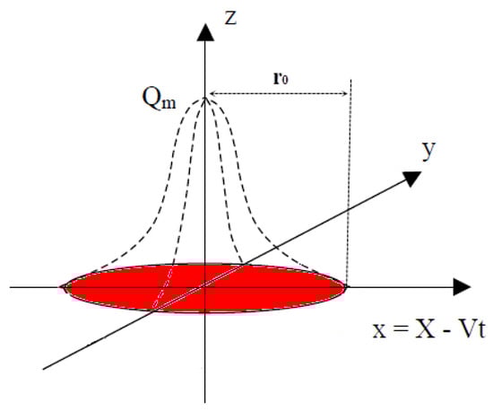
Figure 1.
Surface Gaussian-distributed heat source.
The heat flux input is as shown:
where is the arc efficiency (0.8–0.9), U is the voltage, and I is the electric current.
The heat distribution parameter, denoted as r0, represents the radius of the circular surface heat source as determined through experimental measurements and has been decreased by 5%; it has an influence on the bead width and the penetration depth of the fusion zone [,,].
A convenient measure is the net heat per unit length of the weld, q (J/mm); it can be expressed by
v is the travel sped of the heat source moving along the weld [].
1.2. Prescribed Volumetric Heat Flux Input
In the case of deep penetration fusion welds, a semi-ovaloid (double-ellipsoid) model can be used [].
The Gaussian distribution is widely recognized and commonly employed in numerical modeling to represent the spatial power distribution of electric arc heat sources. Its smooth, bell-shaped profile effectively captures the way heat is concentrated and dissipated during welding processes, making it a standard choice in many simulation studies of arc welding. This approach facilitates accurate prediction of temperature fields and thermal effects in the material being welded. The shape of this source is a combination of two half-ellipses connected to each other with one semi-axis. Power distribution of this ‘double-ellipsoidal’ heat source is described as follows [].
The volumetric Goldak’s heat flux input is shown in Figure 2 and is described by the following equations:
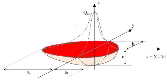
Figure 2.
Goldak’s double-ellipsoid heat source.
With ξ = f for (front) positive x axis, ξ = for (rear) negative x axis.
Where af, ar, b and c are dimensions of semi-ellipsoid axis, coefficients ff and fr represent energy distribution in the front and in the back of the heat source, satisfying the following equations:
They are calculated from c parameter: the values are chosen to be [,]:
af = ½ c and ar = 2 c
Numerical and geometrical values for different heat sources’ parameters are shown in Table 1.

Table 1.
Different parameters for the heat sources.
1.3. Numerical Simulation
In most of the fusion welding processes, a source of concentrated heat and high intensity is applied and moved along the joint position. The temperature value at any point of a solid at any time is calculated by solving the following governing differential equation:
Here, kx, ky and kz are the thermal conductivities in the three directions, is the density, is the specific heat of solid material, and is the internal heat source.
During the welding operation, the material exchanges heat with the surrounding environment by convection and radiation.
Heat losses by convection are given by Newton’s heat transfer law:
Φc = hc(T − T∞)
hc is the coefficient of convection, T the surface temperature of the object, and T∞ the temperature of the surrounding fluid (T∞ = 20 °C).
The heat losses by radiation are
σ: Stefan-Boltzmann constant (σ = 5.7 × 10⁻⁸ Wm−2K−4) and ε the emissivity of the object (ϵ = 0.6) [].
ABAQUS is a software application used for both modeling and analysis of mechanical components and assemblies and visualizing the finite element analysis result [].
The numerical solution was obtained. Two DFLUX user subroutines were developed in Fortran to calculate the surface Gaussian distribution and volumetric Goldak’s heat input to apply the heat flux to the nodes at each sequence as a function of time.
1.4. Assumptions
Main assumptions and features were taken regarding the welding simulation:
- The precise approximation of heat input energy widely affects the accuracy of the thermal distribution model for the values for the two heat input models are obtained through trial and error to yield sufficiently; in our case they were adjusted to get the same heat flux and the maximum temperature as in literature [,,,].
- The butt weld of two plates is modeled in a single pass [].
- The segregation effect and nonequilibrium solidification were neglected.
- All the material properties are described until the liquid phase of metal. When the material is liquid, the related rigidity and resistance are negligible, but both yielding strength and Young’s modulus were limited to small values (5 MPa and 0.1 GPa, respectively) to reduce computation time; the thermal expansion coefficient was considered very small in order to avoid computation divergence [].
- The thermal conductivity is considered as transverse isotropic which increases heat exchanges in the welding direction (λ = 60 Wm−1 K−1 in the welding direction and λ = 30 Wm−1 K−1 in the other directions) [].
hc = 15 Wm−2 K−1 was used for all the surfaces not influenced by the shielding gas, and, hc = 242 Wm−2 K−1 was used for a part of the top surface under the nozzle of the welding gun [].
- The vaporization of the metal is not taken into consideration but only the fusion process is considered.
- The fluid flow in the molten weld pool has not been considered [].
- Elastic–plastic strain and thermal strain are inseparable.
- Thermal properties and stresses/strains related to temperature change linearly in small time increments [].
2. Materials and Methods
2.1. Thermal Simulation of Plate Butt Joint Welding
Geometry Model and Meshing
The single-pass welding process of butt-weld joint of INC 738 LC Ni superalloy was simulated using a rectangular plate with 50 mm × 60 mm × 3 mm as dimensions. Since the welded plate taken for investigation was symmetrical, the symmetry axis was at the plate center. The model coordinate system and mesh divisions are shown in Figure 3 and Figure 4. The plate meshing was composed of 44,400 continuous solid three-dimensional linear standard elements (C3D8RT).
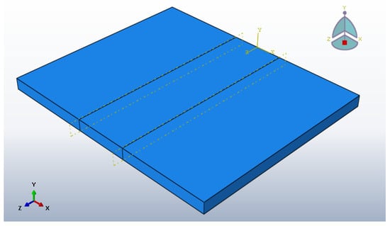
Figure 3.
The model coordinates and partitions.
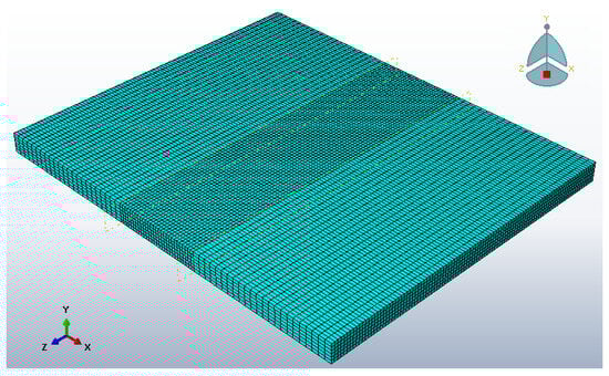
Figure 4.
Mesh model used for analysis.
C3D8RT: An 8-node thermally coupled brick element with trilinear interpolation for both displacement and temperature fields was employed, incorporating reduced integration and hourglass control to enhance computational efficiency and numerical stability.
A refined mesh with element dimensions of 0.5 mm × 0.5 mm × 0.5 mm is employed in the welding region to ensure precise application and accurate distribution of the heat flux.
2.2. Analysis Organisation
2.2.1. Step and Interaction
In this section, a sequentially coupled thermo-elastic–plastic finite element computational procedure is developed to calculate the temperature fields, welding residual stresses, and welding deformations.
A Coupled Temperature-Displacement step is created in order to conduct the analysis for welding and cooling operations. Interactions between the weld pool on the top plates’ surfaces and the surrounding were assumed by attribution of film convection coefficient and radiation coefficient.
2.2.2. Load and Boundary Conditions
The ambient temperature (20 °C) was attributed to the unwelded exterior surfaces of plates as boundary conditions. The thermal load is applied to the weld joint using a surface heat flux based on a Gaussian distribution, while a volumetric heat source is employed in accordance with Goldak’s double-ellipsoidal model. In the mechanical finite element simulation to compute the stress and distortion distributions, boundary constraints are applied to the plate. It was fixed as a cantilever beam to observe the mechanical behavior during and after the welding process to prevent rigid body motion but allow the plate to deform [].
2.2.3. Job Execution
After the job was checked for errors and to verify the data, the results can be visualized and analyzed after execution of submitting the job.
D. Calculation time: After submitting the time needed for the calculation of all the steps was taken into consideration, the total time calculation for the Gaussian distribution was so longer as for Goldak’s heat input.
2.3. Welding Parameters and Material Model
For the current study, the TIG welding process parameters were kept constant for both the surface distribution and volumetric heat input and they are shown in Table 2.
Table 2.
TIG welding process parameters.
2.4. Material Thermophysical Properties
The temperature-dependent properties of the cast INC 738LC alloy, including specific heat capacity, thermal conductivity, and thermomechanical characteristics, were obtained from the literature sources [,,]. These properties are essential for accurately simulating the thermal and mechanical behavior of the alloy during welding. For clarity and better visualization, the variations of these properties as functions of temperature have been plotted and are presented in Figure 5 and Figure 6. These graphs illustrate how the material’s behavior evolves with increasing temperature, which is critical for the fidelity of the numerical model.
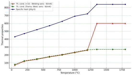
Figure 5.
Thermal properties of INC 738 LC Ni superalloy.
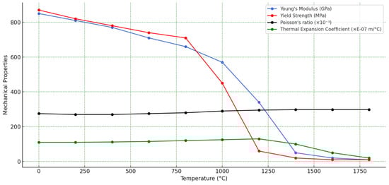
Figure 6.
Thermomechanical properties of INC 738 LC Ni superalloy.
The other material properties that were essential for completing all the numerical calculations in this study have been gathered and summarized in Table 3. These properties, which complement those described earlier, play a crucial role in ensuring the accuracy and reliability of the simulation results.
Table 3.
Material properties.
2.5. Metallurgical Analysis
Fundamental studies have investigated the effect of solidification parameters on the microstructure of Ni-based superalloys. Among various microstructural characteristics, primary dendrite arm spacing (PDAS) λ1 impacts the basic transport phenomena in the mushy zone, and regarding secondary dendrite arm spacing (SDAS) λ2, both have a strong effect on the mechanical properties of these materials []. It was reported that PDAS and SDAS are determined by processing parameters such as thermal gradient (G) and solidification growth rate (R). They are calculated from the temperature field [,,].
Dendrite arm spacings are correlated with the cooling rate (GR) in the Ni superalloy INC 738 LC by the following relationships []:
With G in (K/mm), R in (mm/h).
Mechanical Analysis
When structures are manufactured by welding, a non-uniform temperature distribution is produced. This heat distribution initially induces rapid thermal expansion, followed by thermal contraction in the weld zone and adjacent regions, leading to non-uniform plastic deformation and the development of residual stresses within the weldment upon cooling [,].
The total strain (distortion) next welding can be composed by
These components correspond, respectively, to elastic, plastic, and thermal strains.
The elastic strain is formulated based on isotropic Hooke’s law, incorporating temperature-dependent variations in Young’s modulus and Poisson’s ratio. The plastic strain component is represented using a constitutive plasticity model characterized by the Von Mises yield criterion, also accounting for temperature-dependent material behavior []. The thermomechanical properties adopted in the simulation are presented in Figure 6.
After incorporating a viscous component into the constitutive model to represent the alloy’s behavior at elevated temperatures, the results revealed that a lower viscous contribution leads to reduced deviations, indicating improved agreement with expected thermal-mechanical responses [].
The use of an elastoplastic behavior model (EP) allows us to obtain better results regarding the estimation of the residual strains compared to an elastoviscoplastic (EVP) model [,,].
Danis et al. [] stated that hot cracking occurs in the TIG welding of the INC 738 LC, if the calculated stresses range between 360 MPa and 550 MPa for the used welding conditions. This allows us to map the danger of hot cracking zones in the welded parts.
3. Results and Discussions
3.1. Heat Flux
The Gaussian heat distribution and the Goldak’s heat input and their temperature fields are represented in Figure 7 and Figure 8. The Gaussian distribution heat flux is greater than the Goldak’s input.
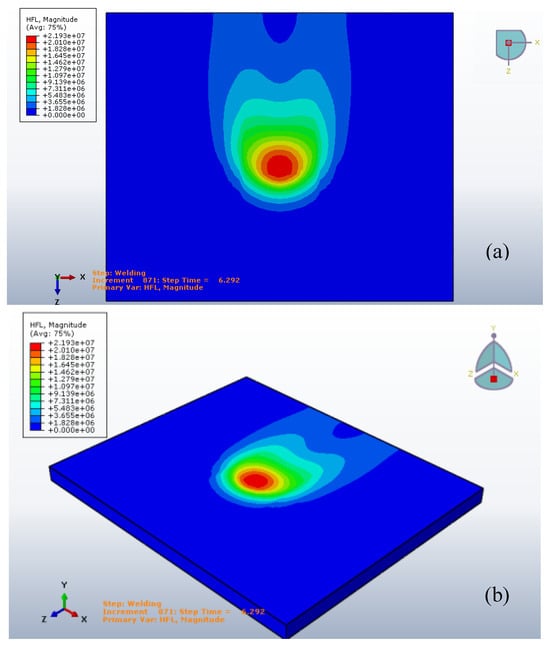
Figure 7.
The Gaussian heat distribution at 6.292 s, (a) top view, (b) isometric view.
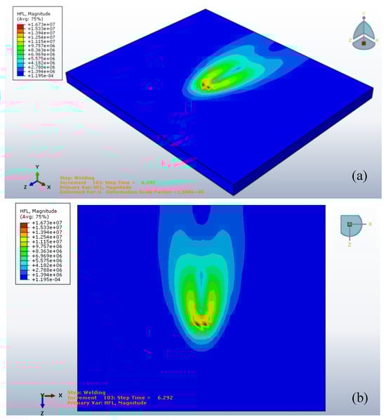
Figure 8.
The Goldak’s heat flux at 6.292 s, (a) top view, (b) isometric view.
3.2. Temperature Distributions
The temperature distributions of the Gaussian heat distribution and the Goldak’s input are represented in Figure 9 and Figure 10. The maximum temperature of the Goldak’s input is less than the Gaussian heat distribution as made evident in the assumptions.
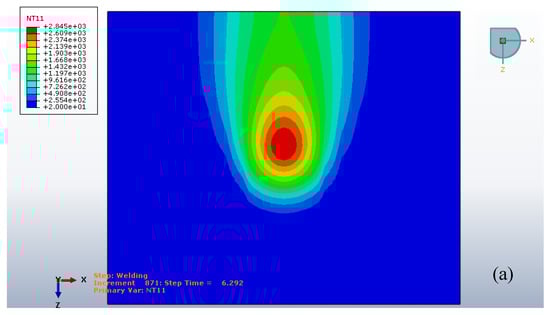
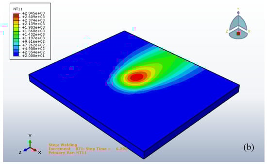
Figure 9.
The temperature distribution of the Gaussian heat distribution at 6.292 s, (a) top view, (b) isometric view.
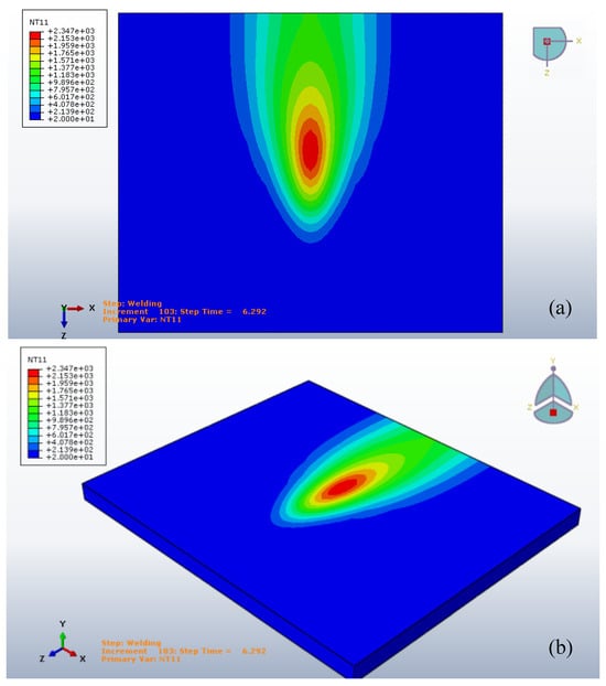
Figure 10.
The temperature distribution of Goldak’s heat input at 6.292 s, (a) top view, (b) isometric view.
3.3. Metallurgical Analysis (Solidification Parameters)
The experimentally validated finite element model was employed using the Smitweld TCS 1405 thermal cycle simulator during welding simulation thermal cycles [].
Many points (five) were chosen from the fusion line to the center line as shown in Figure 11a,b which show a plot of thermal cycle at a point (A-fusion line) to calculate the cooling rate around the welding pool.
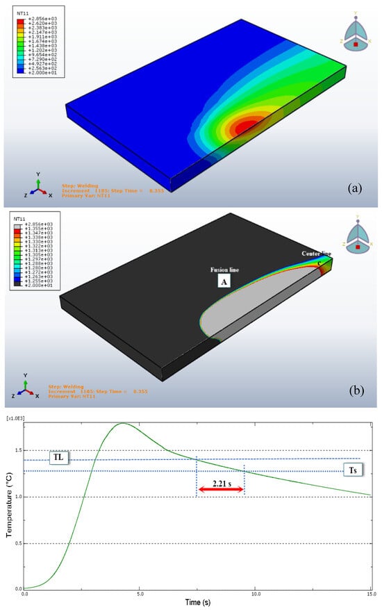
Figure 11.
Weld profiles and thermal cycle of Gaussian distribution for weld at 8.355 s and fusion line, (a) weld profiles and the solidification temperature range for weld at 8.355 s, (b) thermal cycle and cooling times calculated at the documented nodes located at the fusion line (Point A).
Prediction of Cooling Rates and Dendrite Arm Spacings
Figure 11a shows the thermal field in the welding operation with temperature limits (TL and Ts) for Gaussian distribution.
Figure 12 illustrates the predicted cooling rates and dendrite arm spacings around a weld pool at 8.355 s using a Gaussian distribution model. In Figure 12a, the graph shows the variation in cooling rate with normalized distance from the fusion line (Point A) to the center line of the weld (Point C). The cooling rate increases steadily from approximately 630,000 K/s near the fusion line to about 940,000 K/s at the center, indicating higher thermal gradients and faster solidification toward the weld center. Figure 12b displays the predicted dendrite arm spacings, where λ1 (primary dendrite arm spacing) slightly decreases from around 27 µm at the fusion line to about 24 µm near the center. Meanwhile, λ2 (secondary dendrite arm spacing) remains relatively constant at approximately 3–4 µm across the weld pool. These trends suggest that the finer microstructure observed toward the weld center is a result of the higher cooling rates experienced in that region.
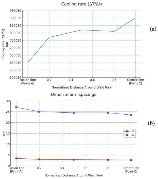
Figure 12.
Cooling rates and dendrite arm spacings of Gaussian distribution for weld at 8.355 s, (a) predicted cooling rates around weld pool, (b) predicted dendrite arm spacings.
Figure 13 shows the weld profiles and thermal cycle during welding at 8.350 s using Goldak’s heat input model. Figure 13a illustrates the temperature distribution and solidification range around the weld. Figure 13b presents the thermal cycle at the fusion line (Point A), showing a 1.92-second solidification time between the liquidus (TL) and solidus (TS) temperatures.
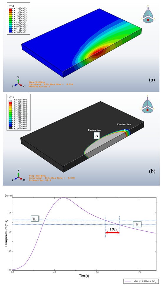
Figure 13.
Weld profiles and thermal cycle of Goldak’s heat input for weld at 8.350 s and fusion line; (a) weld profiles and the solidification temperature range for weld at 8.350 s; (b) thermal cycle and cooling times calculated at the documented nodes located at the fusion line (Point A).
Figure 14 illustrates the predicted cooling rates and dendrite arm spacings around the weld pool at 8.350 s using Goldak’s heat input model. In Figure 14a, the cooling rate initially decreases slightly, then increases significantly, reaching a peak near the normalized distance of 0.8 before slightly declining toward the center line. Figure 14b shows the dendrite arm spacings, where the primary spacing (λ1) decreases from the fusion line toward the weld center, indicating finer microstructure in regions with higher cooling rates. The secondary spacing (λ2) remains relatively constant across the weld. These results highlight the inverse relationship between cooling rate and dendrite arm spacing.
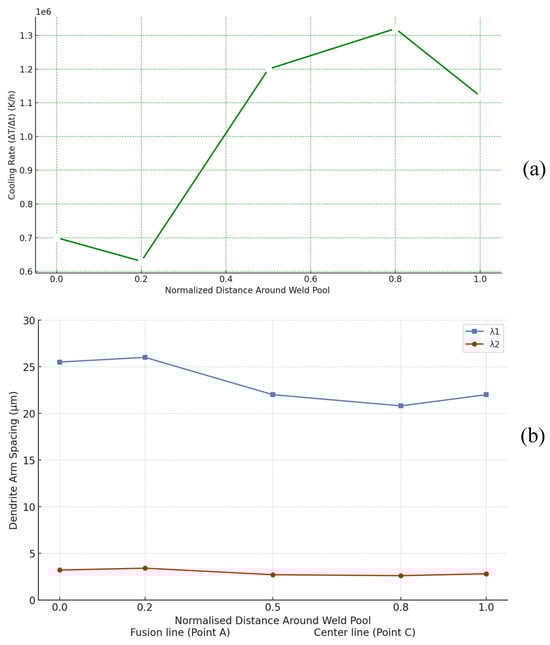
Figure 14.
Cooling rates and dendrite arm spacings of Goldak’s heat input for weld at 8.350 s, (a) predicted cooling rates around weld pool, (b) predicted dendrite arm spacings.
As a comparison between the Gaussian heat distribution and the Goldak’s heat input in the metallurgical analysis, we can prove the following:
- It can be clearly seen that in all welds the cooling rate is the highest at the center line.
- The dendrite arm spacings are approximatively similar; the maximum dendrite arm spacing errors are 3.5 µm for λ1 and 0.5 µm for λ2 between the two heat sources, as shown in Figure 15.
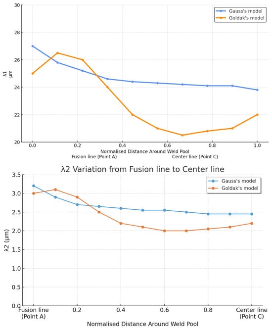 Figure 15. Predicted dendrite arm spacings for welds at 8.350 s.
3.4. Mechanical Analysis
3.4.1. Residual Stresses Calculation
Residual stresses are evaluated using the same mesh that was used for calculating the temperatures.
Figure 16 presents the transverse residual stresses of a point from the top surface at 8.355 s from the welding line obtained by the Gaussian distribution. The stress curve increases from base metal to reach a maximum value 0.8 GPa in the (heat-affected zone) HAZ zone; the gap between the two maximum stresses is around 0.012 (m); afterward, the stress curve decreases to 0.6 GPa in the FZ (fusion zone).
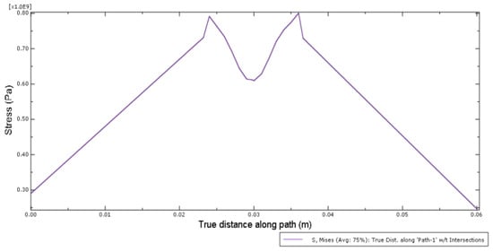
Figure 16.
The Gaussian distribution transverse residual stresses at 8.355 s.
By using the Goldak’s heat input, the transverse residual stresses in a point at 8.35 s from the welding line are shown in Figure 17. The stresses curve raises from base metal to attain a maximum value 1.1 GPa in the (heat-affected zone) HAZ zone; the two maximum stresses distance is around 0.007 (m); after that in the FZ (fusion zone), the stresses curve reduces to 0.78 GPa.
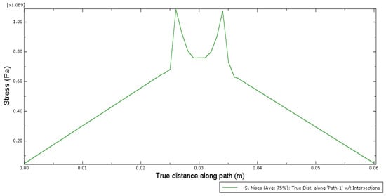
Figure 17.
The Goldak’s heat input transverse heat input at 8.35 s.
Figure 18 compares transverse stress distributions for Gauss’s and Goldak’s heat input models. The transposition of the transverse stresses in both heat inputs shows the changes. Gauss’s model shows a smoother, lower peak stress profile, while Goldak’s model produces sharper, higher stress peaks, indicating more localized heat effects.
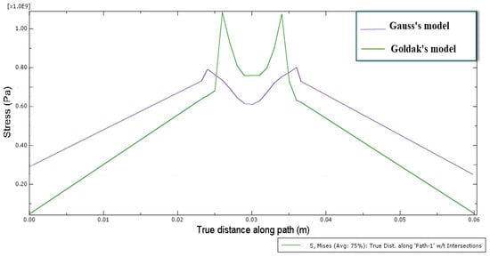
Figure 18.
The transverse stresses superposition for the two heat input models.
Through the use of the stress limitations cited as a hot crack criterion, it is possible to map the crack-sensitive areas as shown in Figure 19a for Gaussian distribution and Figure 19b for Goldak’s heat input; the cracking risk areas at the end of the welding operation are given in Figure 20; for both of the heat sources, they are situated in the HAZ zones near the base metal.
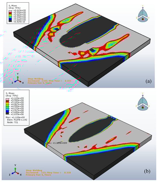
Figure 19.
Von Mises stresses fields, (a) the Gaussian distribution at 8.355 s, (b) the Goldak’s heat input at 8.350 s.
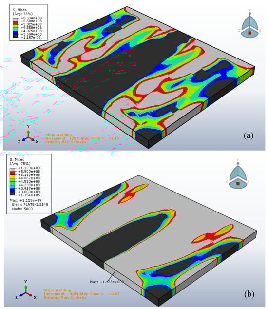
Figure 20.
Von Mises stresses distribution at the end of welding operation, (a) the Gaussian distribution, (b) the Goldak’s heat input.
3.4.2. Displacement Fields Computation
Displacement fields were magnified (by using a scale factor = 10) to show the distortions of the welded plates as shown in isometric view, in Figure 21 illustrate the displacement magnitude resulting from thermal and mechanical effects during the welding process of a metal plate. Figure 21a presents a longitudinal side view of the welded joint, showing the distribution of deformation along the X-axis. The highest displacement, approximately 2.118 × 10⁻⁴, occurs at the weld center, with a gradual reduction toward the edges, as indicated by the color gradient from red (maximum) to blue (minimum). Figure 21b offers a three-dimensional perspective of the deformation, highlighting the out-of-plane distortion relative to the initial surface profile. The region near the weld exhibits a noticeable bulge, indicating localized expansion due to heat input. The labeled arrow marks the initial undeformed surface, clearly demonstrating the extent of warping. Figure 21c provides a top-down view, illustrating the deformation pattern in the transverse (Z) and depth directions. The contour distribution reveals a symmetrical spread of displacement from the weld centerline, with the intensity diminishing outward, reflecting the thermal gradient and material response in the heat-affected zone.
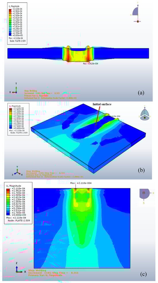
Figure 21.
The gaussian distribution displacement at 8.355 s, (a) Longitudinal deformation distribution (U magnitude) along the welded joint, (b) Three-dimensional view of deformation with reference to the initial surface profile, (c) Top view of the deformation pattern showing transverse and depth-wise displacement gradients.
Figure 22 depicts the displacement distribution in a welded plate during the welding process. Figure 22a shows a side view, where the maximum vertical deformation occurs at the weld center due to localized thermal expansion. Figure 22b presents a 3D perspective, highlighting how the displacement spreads from the weld line. Figure 22c provides a top view, revealing an elongated deformation pattern along the welding path. These views collectively demonstrate the thermal distortion effects induced by the welding heat source.
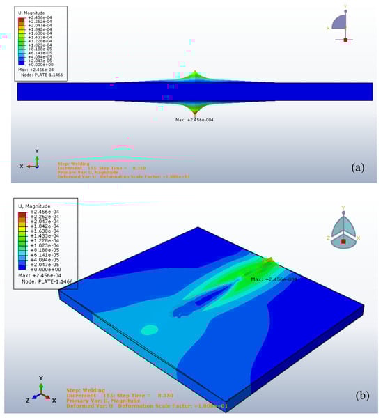
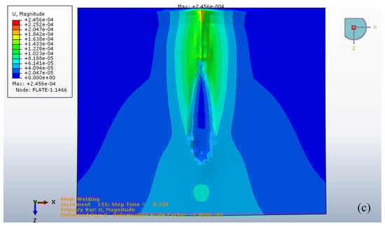
Figure 22.
The Goldak’s heat input displacement at 8.350 s, (a) Transverse Displacement Profile of Welded Plate (Side View), (b) 3D Perspective View of Displacement Distribution During Welding, (c) Top View of Displacement Magnitude Induced by Welding Heat Source.
4. Conclusions
In this study, a transient heat transfer equation for a solid body, representing the welding simulation of a Ni superalloy INC 738 LC plate, was solved using the finite element method with the ABAQUS solver. The main conclusions are as follows:
- Two types of heat sources, surface distribution and volumetric input, were employed in the simulation.
- Thermal fields and heat fluxes were determined for both heat source models.
- Solidification parameters, such as dendrite arm spacings, were calculated based on predicted cooling rates at various points around the weld pools; these values were similar for both heat input methods.
- Transverse residual stresses were evaluated, and a hot cracking criterion was established to identify regions susceptible to hot cracking.
- The maximum transverse stress recorded was 1.1 GPa in the heat-affected zone (HAZ) for the Goldak heat input model.
- Distortions and strains of the welded plate were estimated for both heat sources.
- At the conclusion of the welding process, the Gaussian heat source resulted in a significant expansion of the fusion zone (FZ), as observed in the mapped residual stresses and displacement values, compared to the Goldak heat input.
Author Contributions
Conceptualization, C.S. and S.A.; methodology, C.S.; software, M.-S.C.; validation, A.B.; formal analysis, S.Z. and B.M.; data curation, S.A. and B.M.; writing—original draft preparation, C.S., A.B. and B.M.; writing—review and editing, B.M.; visualization, C.S. and B.M.; supervision, C.S., S.Z. and S.A.; project administration, A.B.; funding acquisition, C.S., M.-S.C. and S.Z. All authors have read and agreed to the published version of the manuscript.
Funding
This research received no external funding.
Data Availability Statement
The raw data supporting the conclusions of this article will be made available by the authors on request.
Conflicts of Interest
The authors declare no conflicts of interest.
References
- Arora, H.; Singh, R.; Brar, G.S. Thermal and structural modelling of arc welding processes: A literature review. Meas. Control 2019, 52, 955–969. [Google Scholar] [CrossRef]
- Zhang, X.; Zhang, W.; Bian, S.; Zhao, P. A calculation method of solidification parameter threshold for welding microstructure evolution. Mater. Lett. 2023, 330, 133399. [Google Scholar] [CrossRef]
- Danis, Y.; Lacoste, E.; Arvieu, C. Numerical modeling of Inconel 738LC deposition welding: Prediction of residual stress-induced cracking. J. Mater. Process. Technol. 2010, 210, 2053–2061. [Google Scholar] [CrossRef]
- Tamil Prabakaran, S.; Sakthivel, P.; Shanmugam, M.; Satish, S.; Muniyappan, M.; Shaisundaram, V.S. Modelling and Experimental Validation of TIG Welding of INCONEL 718. Mater. Today Proc. 2021, 37, 1917–1931. [Google Scholar] [CrossRef]
- Lundbäck, A. Modelling and Simulation of Welding and Metal Deposition. Ph.D. Thesis, Luleå University of Technology, Department of Applied Physics and Mechanical Engineering, Luleå, Sweden, 2010. [Google Scholar]
- Ghafouri, M.; Ahola, A.; Ahn, J.; Björk, T. Numerical and Experimental Investigations on the Welding Residual Stresses and Distortions of the Short Fillet Welds in High Strength Steel Plates. Eng. Struct. 2022, 260, 114269. [Google Scholar] [CrossRef]
- Wang, W.; Lin, W.; Yang, R.; Wu, Y.; Li, J.; Zhang, Z.; Zhai, Z. Mesoscopic Evolution of Molten Pool during Selective Laser Melting of Superalloy Inconel 738 at Elevating Preheating Temperature. Mater. Des. 2022, 213, 110355. [Google Scholar] [CrossRef]
- Bidron, G.; Doghri, A.; Malot, T.; Fournier-dit-Chabert, F.; Thomas, M.; Peyre, P. Reduction of the Hot Cracking Sensitivity of CM-247LC Superalloy Processed by Laser Cladding Using Induction Preheating. J. Mater. Process. Technol. 2020, 277, 116461. [Google Scholar] [CrossRef]
- Hansen, J.L. Numerical Modelling of Welding Induced Stresses. Ph.D. Thesis, Technical University of Denmark, Department of Manufacturing Engineering and Management, Kongens Lyngby, Denmark, 2003. [Google Scholar]
- Goldak, J.; Chakravarti, A.; Bibby, M. A new finite element model for welding heat sources. Metall. Trans. B 1984, 15, 299–305. [Google Scholar] [CrossRef]
- Teixeira, P.R.D.F.; de Araújo, D.B.; da Cunha, L.A.B. Study of the Gaussian distribution heat source model applied to numerical thermal simulations of TIG welding processes. Ciênc. Eng. 2014, 23, 115–122. [Google Scholar]
- Piekarska, W.; Kubiak, M.; Saternus, Z. Application of Abaqus to analysis of the temperature field in elements heated by moving heat sources. Arch. Foundry Eng. 2010, 10, 177–182. [Google Scholar]
- Rocha, E.J.F.; Antonino, T.d.S.; Guimarães, P.B.; Ferreira, R.A.S.; Barbosa, J.M.A.; Rohatgi, J. Modeling of the temperature field generated by the deposition of weld bead on a steel butt joint by FEM techniques and thermographic images. Mater. Res. 2018, 21, e20160796. [Google Scholar] [CrossRef]
- Esfahani, M.M. Welding Simulation of Steels Welded with Low Transformation Temperature (LTT) Filler Materials. Master’s Thesis, Chalmers University of Technology, Gothenburg, Sweden, 2016. [Google Scholar]
- Perić, M.; Tonković, Z.; Rodić, A.; Surjak, M.; Garašić, I.; Boras, I.; Švaić, S. Numerical Analysis and Experimental Investigation of Welding Residual Stresses and Distortions in a T-Joint Fillet Weld. Mater. Des. 2014, 53, 1052–1063. [Google Scholar] [CrossRef]
- Perić, M.; Stamenković, D.; Milković, V. Comparison of residual stresses in butt-welded plates using software packages Abaqus and Ansys. Sci. Tech. Rev. 2010, 60, 22–26. [Google Scholar]
- Kumar, P.; Kumar, R.; Arif, A.; Veerababu, M. Investigation of numerical modelling of TIG welding of austenitic stainless steel (304L). Mater. Today Proc. 2020, 27, 1636–1640. [Google Scholar] [CrossRef]
- Yang, X.; Yan, G.; Xiu, Y.; Yang, Z.; Wang, G.; Liu, W.; Li, S.; Jiang, W. Welding temperature distribution and residual stresses in thick welded plates of SA738Gr.B through experimental measurements and finite element analysis. Materials 2019, 12, 2436. [Google Scholar] [CrossRef] [PubMed]
- Bonifaz, E.A.; Indacochea, J.E. Thermo-mechanical modeling of single high-power diode laser welds. In Proceedings of the Third LACCEI International Latin American and Caribbean Conference for Engineering and Technology (LACCET’ 2005): Advances in Engineering and Technology: A Global Perspective, Cartagena, Colombia, 8–10 June 2005; pp. 1–9. [Google Scholar]
- Zhang, W.; Lin, L.; Taiwen, H.; Xinbao, Z.; Min, Q.; Zhuhuan, Y.; Hengzhi, F. Influence of directional solidification variables on primary dendrite arm spacing of Ni-based superalloy DZ125. China Foundry 2009, 6, 300–304. [Google Scholar]
- Milenkovic, S.; Rahimian, M.; Sabirov, I.; Maestro, L. Effect of solidification parameters on the secondary dendrite arm spacing in MAR M-247 superalloy determined by a novel approach. In MATEC Web of Conferences; EDP Sciences: Les Ulis, France, 2014. [Google Scholar]
- Blecher, J.J.; Palmer, T.A.; Debroy, T. Solidification map of a nickel-base alloy. Metall. Mater. Trans. A 2014, 45, 2142–2151. [Google Scholar] [CrossRef]
- Kermanpur, A.; Varahraam, N.; Engilehei, E.; Mohammadzadeh, M.; Davami, P. Directional solidification of Ni-base superalloy IN738LC to improve creep properties. Mater. Sci. Technol. 2000, 16, 579–586. [Google Scholar] [CrossRef]
- Nuraini, A.A.; Zainal, A.S.M.; Azmah Hanim, M.A. The effect of welding process parameters on temperature and residual stress in butt-joint weld of robotic gas metal arc welding. Aust. J. Basic Appl. Sci. 2013, 7, 814–820. [Google Scholar]
- Deng, D.; Murakawa, H. Prediction of welding distortion and residual stress in a thin plate butt-welded joint. Comput. Mater. Sci. 2008, 43, 353–365. [Google Scholar] [CrossRef]
- Pichot, F. Development of a Numerical Method for Predicting the Dimensions of a TIG Weld Bead: Application to Cobalt and Nickel Base Superalloys. Ph.D. Thesis, University of Bordeaux, Bordeaux, France, 2012. [Google Scholar]
- Siguerdjidjene, H.; Houari, A.; Madani, K.; Amroune, S.; Mokhtari, M.; Mohamad, B.; Campilho, R. Predicting damage in notched functionally graded materials plates through extended finite element method based on computational simulations. Frat. Integrità Strutt. 2024, 18, 1–23. [Google Scholar] [CrossRef]
- Khayoon, S.; Ameen, N.H.; Fadheel, K.I.; Anead, A.M.; Mhabes, H.E.; Mohamad, B. An experimental artificial neural network model: Investigating and predicting effects of quenching process on residual stresses of AISI 1035 steel alloy. J. Harbin Inst. Technol. 2024, 31, 78–92. [Google Scholar]
- Bonifaz, E.A.; Richards, N.L. Modeling Cast IN-738 Superalloy Gas Tungsten Arc Welds. Acta Mater. 2009, 57, 1785–1794. [Google Scholar] [CrossRef]
- Elhadi, A.; Amroune, S.; Zaoui, M.; Mohamad, B.; Bouchoucha, A. Experimental investigations of surface wear by dry sliding and induced damage of medium carbon steel. Diagnostyka 2021, 22, 3–10. [Google Scholar]
Disclaimer/Publisher’s Note: The statements, opinions and data contained in all publications are solely those of the individual author(s) and contributor(s) and not of MDPI and/or the editor(s). MDPI and/or the editor(s) disclaim responsibility for any injury to people or property resulting from any ideas, methods, instructions or products referred to in the content. |
© 2025 by the authors. Licensee MDPI, Basel, Switzerland. This article is an open access article distributed under the terms and conditions of the Creative Commons Attribution (CC BY) license (https://creativecommons.org/licenses/by/4.0/).