A Deep Learning-Based CNN-LSTM Framework for Constitutive Parameter Inversion in Alloy Gradient-Grained Materials

Abstract

Alloy gradient-grained structures (represented by copper as a typical single-phase face-centered cubic (FCC) metal), known for their superior mechanical properties such as enhanced strength, ductility, and fatigue resistance, have become increasingly important in aerospace and automotive industries. These alloys are often fabricated using advanced processing techniques such as laser welding, electron beam melting, and controlled cooling, which induce spatial gradients in grain size and optimize material properties by overcoming the traditional strength–ductility trade-off. In this study, a deep learning-based inversion framework combining Convolutional Neural Networks (CNN) and Long Short-Term Memory (LSTM) networks is proposed to efficiently predict key constitutive parameters, such as the initial critical resolved shear stress and hardening modulus, in alloy gradient-grained structures. The model integrates spatial features extracted from strain-field sequences and grain morphology images with temporal features from loading sequences, providing a comprehensive solution for path-dependent mechanical behavior modeling. Trained on high-fidelity Crystal Plasticity Finite Element Method (CPFEM) simulation data, the proposed framework demonstrates high prediction accuracy for the constitutive parameters. The model achieves an error margin of less than 5%. This work highlights the potential of deep learning techniques for the efficient and physically consistent identification of constitutive parameters in alloy gradient-grained structures, offering valuable insights for alloy design and optimization.

1. Introduction

In recent years, with the increasing demand for structural lightweighting, gradient-grained materials have attracted significant attention in the aerospace and automotive industries. Gradient-grained materials exhibit excellent mechanical properties, including enhanced strength, ductility, and fatigue resistance, which make them one of the key materials for advanced applications [1,2]. The fabrication of gradient-grained materials typically relies on advanced metal processing techniques. For example, laser welding, laser melting deposition, electron beam melting, and the control of cooling rates can all induce spatial gradients in grain size within the material [3,4]. These processes achieve precise control over heat input, cooling rates, and alloy compositions to ensure the formation of distinct microstructures in different regions, thereby optimizing the mechanical performance of the material. By manipulating grain size and distribution, gradient-grained materials can achieve higher strength or ductility in designated regions, thus overcoming the traditional strength–ductility trade-off and enhancing overall performance.

Compared to materials with uniform grain size distribution, gradient-grained materials can achieve a better balance between strength and ductility. In gradient-grained microstructures, coarse grains are beneficial for bearing higher stresses and providing more space for slip during deformation, while fine grains enhance resistance to slip and thereby hinder dislocation motion. Wu et al. [5] conducted uniaxial tensile tests on gradient-grained interstitial-free (IF) steel and copper plates with different volume fractions of gradient structure, finding that the yield strength of gradient-grained materials was higher than the values predicted by the rule of mixtures. This suggests that gradient structures can lead to synergistic strengthening. Yang et al. [6] performed loading-unloading-reloading experiments on gradient-grained IF steel sheets and found that materials with gradient grain structures exhibit pronounced kinematic hardening. They pointed out that the non-uniform deformation arising from the gradient structure contributes significantly to the synergistic strengthening and toughness of these materials. Lin et al. [7] fabricated gradient-grained nickel with different gradient rates via electroplating, discovering that, under appropriate grain size distributions, the strength and toughness of gradient-grained structures could even exceed those of coarse-grained counterparts. Moreover, they observed that the yield strength and necking strain of nickel with different gradient structures approximately follow a linear decreasing relationship. Zhao et al. [8] developed a constitutive model to simulate and analyze the characteristic kinematic hardening behavior of gradient-structured metals, and their studies revealed that gradient-structured copper exhibits enhanced kinematic hardening, mainly due to the presence of fine grains in the gradient layers.

To investigate the mechanical behavior of gradient-grained materials, the Crystal Plasticity Finite Element Method (CPFEM) [9] has been widely used, providing a powerful means to elucidate slip evolution at the grain scale and its correlation with mechanical properties. CPFEM effectively captures the influence of grain orientation, size, and morphology on local plasticity and microscale stress distribution, offering crucial insights into the synergistic strengthening mechanisms of gradient microstructures. Compared with conventional isotropic models, CPFEM can explicitly simulate grain slip system activation and grain boundary interactions, thus revealing the intrinsic microscale deformation behavior [10].

Several studies have demonstrated its effectiveness in modeling complex microstructures. Zheng et al. established three-dimensional CPFEM–Voronoi models to quantify the effect of grain orientation on macroscopic properties [11], while Liu et al. coupled CPFEM with a phase-field approach to investigate crack initiation in aluminum alloys with grain-size gradients, showing that the coupling between the stress-gradient direction and the grain boundary normal governs crack nucleation [12]. Herath et al. further applied CPFEM within a multiscale framework to additively manufactured titanium alloys, accurately predicting anisotropic stress–strain behavior and microscale strain localization [13].

The accuracy of CPFEM simulations, however, depends on predefined constitutive parameters such as the critical resolved shear stress, hardening modulus, and saturation value. These parameters are often identified through iterative “trial-and-error” fitting against experimental results, which becomes inefficient for models involving numerous coupled variables. To address this challenge, recent studies have introduced deep learning (DL) approaches that can efficiently extract complex nonlinear correlations between high-dimensional physical variables and constitutive parameters, offering a promising route for data-driven identification in gradient-textured metals [14].

As a branch of machine learning, deep learning (DL) has undergone a progressive evolution in materials modeling—from static regression modeling, to dynamic sequence learning, and finally to the embedding of physical consistency. In the early stage, DL models were mainly used to construct nonlinear mappings between microstructural images and mechanical parameters. Zeng et al. [15] developed a CNN-based inverse design framework capable of predicting the constitutive parameters of gradient mechanical metamaterials directly from microstructural images, demonstrating the potential of DL for structure–property linkage modeling.

With the increasing awareness of load-path dependency, Guo et al. [16] proposed CPINet, which integrates convolutional neural networks (CNN) with long short-term memory (LSTM) units to process strain field sequences over multiple time steps, achieving dynamic inversion of key constitutive parameters such as yield stress and hardening modulus. This marked a shift from static regression toward sequence-based learning of deformation evolution.

More recently, efforts have focused on embedding physical consistency into DL frameworks to enhance interpretability and generalization. Hu et al. [17] introduced a cross-scale temporal graph neural network that integrates microstructural descriptors with time-evolution behavior, enabling physically consistent modeling of polycrystalline deformation across scales. These developments collectively highlight the growing capability of DL to capture the complex, path-dependent mechanical responses of gradient-grained materials.

Recent studies have extended deep learning (DL) to the inverse design and parameter identification of gradient or functionally graded materials—e.g., Zeng et al. [15] using CNNs for microstructure–property mapping, Li et al. [18] for DL-assisted design of graded auxetic lattices, and Jadoon et al. [19] with physics-augmented networks for anisotropic microstructures. In parallel, Alshammari et al. [20] proposed a practical method for producing functionally graded materials by varying exposure time via photo-curing 3D printing, offering a complementary manufacturing pathway for validating gradient models through experimental synthesis. Despite these advances, current CPFEM–DL applications remain dominated by forward prediction of mechanical properties, while the inverse identification of constitutive-parameter spectra—particularly for gradient-grained alloys—remains underexplored. To address this gap, the present study develops a coupled CNN-LSTM framework for spatiotemporal inversion of constitutive parameter fields, integrating multimodal data (gradient metallographs, time-series strain fields, and loading-path features) to enhance interpretability and reliability.

The proposed framework provides practical guidance for the performance optimization and digital-twin design of gradient-grained alloys used in aerospace and high-performance engineering structures. Gradient-grained structures have been widely used in aerospace components such as turbine blades, fuselage skins, and thermal protection layers, offering an effective balance between high strength and ductility. Rapid prediction of local constitutive parameters in such materials can significantly accelerate performance-oriented material design [21,22].

This study develops a deep-learning inversion framework that fuses multimodal inputs and temporal modeling to improve both efficiency and physical consistency in identifying key constitutive parameters of gradient-grained structures. The model predicts the spatial fields of the initial critical resolved shear stress (τ₀) and hardening modulus (h), characterizing their intrinsic variation along the grain-size gradient and elucidating the impact on macroscopic strain evolution. Unlike previous studies that mainly focused on geometrical or microstructural gradients, this study develops an inverse identification framework for the constitutive-parameter fields (τ₀, h) in gradient-grained alloys by coupling a CNN-LSTM architecture. The model integrates spatial features extracted from strain-field sequences and grain morphology images with temporal features obtained from strain-field and loading sequences as multimodal inputs, while the attention-weight visualization is employed to interpret the respective contributions of strain fields, loading paths, and grain morphology to parameter identification.

The remaining sections of this paper are organized as follows: Section 2 presents an extended crystal plasticity finite element (CPFE) model that incorporates grain size and orientation, which is subsequently used to simulate the effect of grain size gradients on the plastic deformation of alloys. Section 3 introduces a CNN-LSTM-based framework for the inversion of crystal plasticity parameters. Section 4 discusses the feasibility and applicability of the proposed approach by evaluating the performance of the CNN-LSTM model in the inversion of constitutive parameters. Finally, Section 5 of this study are summarized.

2. Materials and Methods

In order to investigate the effects of grain size and orientation gradients on the macroscopic mechanical properties of alloys with gradient grain distributions, this section first reviews the classical crystal plasticity theory for gradient-grained structures, and then simplifies the crystal plasticity constitutive model based on the Hall–Petch effect. The model focuses on the influence of grain size and orientation on the plastic deformation behavior of materials, providing a theoretical foundation for the subsequent deep learning-based inversion of constitutive parameters.

Subsequently, a CPFE model for gradient-grained structures is employed. Using ABAQUS software (2022), simulations are conducted to examine the impact of various grain size gradients on the plastic deformation behavior of alloys with gradient grain distributions. These simulations verify the relationships among grain size, yield strength, and hardening modulus, thereby providing essential data support for the development of the subsequent deep learning model.

2.1. Classical Crystal Plasticity Theory

The crystal plasticity (CP) theory attributes the macroscopic plastic deformation of metallic materials to the accumulation of shear deformation events on individual slip systems. It elucidates the macroscopic mechanical behavior of metals at the mesoscale, offering a clear physical interpretation.

Hill [23] and Rice [24] provided the mathematical formulations for the kinematics and deformation geometry of crystals. On this basis, the total deformation of a crystal can be described as the accumulation of both elastic and plastic deformations. The deformation gradient F can thus be decomposed into elastic and plastic parts as follows [25,26]:

$$\mathbf{F}={\mathbf{F}}^{\mathrm{e}}\cdot {\mathbf{F}}^{\mathrm{p}}$$

(1)

where F^e represents the elastic deformation gradient associated with lattice stretching (distortion) and rigid body rotation, while F^p denotes the plastic deformation gradient arising from shear deformation due to slip within the crystal.

At this stage, the deformation rate gradient is decomposed into two components: one associated with slip, and the other corresponding to lattice distortion combined with rigid body rotation.

The deformation rate gradient L can also be decomposed into an elastic part L^e and a plastic part L^p, as expressed by the following equation:

$$\mathbf{L}=\dot{\mathbf{F}}\cdot {\mathbf{F}}^{-1}={\mathbf{L}}^{\mathrm{e}}+{\mathbf{L}}^{\mathrm{p}}$$

(2)

where

$${\mathbf{L}}^{\mathrm{e}}={\dot{\mathbf{F}}}^{\mathrm{e}}\cdot {\mathbf{F}}^{\mathrm{e}-1}$$

(3)

$${\mathbf{L}}^{\mathrm{p}}={\dot{\mathbf{F}}}^{\mathrm{p}}\cdot {\mathbf{F}}^{\mathrm{p}-1}={\displaystyle {\sum }_{\alpha =1}^{\mathrm{N}}{\dot{\gamma }}^{\alpha }}{\mathbf{s}}^{\alpha }\otimes {\mathbf{n}}^{\alpha }$$

(4)

After crystal deformation, the corresponding deformation rate tensor for slip system α, P^α, is defined as follows [9]:

$${\mathbf{P}}^{\alpha }={\displaystyle \frac{1}{2}}\left({\mathbf{s}}^{\alpha }\otimes {\mathbf{m}}^{\alpha }+{\mathbf{m}}^{\alpha }\otimes {\mathbf{s}}^{\alpha }\right)$$

(5)

Plastic deformation is primarily caused by the activation of slip systems in the crystal. For the α-th slip system, the slip direction is denoted as ${\mathbf{s}}^{\alpha }$, and the slip plane normal as ${\mathbf{m}}^{\alpha }$, which can be expressed as follows:

$$\left\{\begin{array}{c}{\mathbf{s}}^{\alpha }={\mathbf{F}}^{\mathrm{e}}\cdot {\mathbf{s}}_0^{\alpha }\\ {\mathbf{m}}^{\alpha }={\mathbf{m}}_0^{\alpha }\cdot {\mathbf{F}}^{\mathrm{e}-1}\end{array}\right.$$

(6)

where ${\mathbf{s}}_0^{\alpha }$ is the unit vector of the slip direction for the α-th slip system before deformation, and ${\mathbf{m}}_0^{\alpha }$ is the unit normal vector of the slip plane for the α-th slip system. When the lattice undergoes elongation, the unit slip direction vector transforms to ${\mathbf{s}}^{\alpha }$, and the corresponding unit normal vector on the slip plane becomes ${\mathbf{m}}^{\alpha }$.

γ represents the accumulated shear strain over all slip systems, which can be expressed as follows:

$$\gamma ={\displaystyle {\sum }_{\alpha }{\displaystyle {\int }_0^T\left|{\dot{\gamma }}^{\alpha }\right|}}\mathrm{d}\mathrm{t}$$

(7)

where ${\dot{\gamma }}^{\alpha }$ is the plastic shear rate on the α slip system. The slip rate follows a power-law relationship and is related to the strain rate sensitivity, as follows:

$${\dot{\gamma }}^{\alpha }={\dot{\gamma }}_0{\left|{\displaystyle \frac{{\tau }^{\alpha }}{g^{\alpha }}}\right|}^n\cdot \mathrm{s}\mathrm{i}\mathrm{g}\mathrm{n}\left({\tau }^{\alpha }\right)$$

(8)

where ${\dot{\gamma }}_0^{\alpha }$ is the reference shear rate, n is the strain rate sensitivity exponent, τ^α is the resolved shear stress, and g^α is the current shear resistance (also referred to as the critical resolved shear stress).

The resolved shear stress τ^α can be obtained by the double contraction of the Cauchy stress tensor with the deformation rate tensor P^α, as follows:

$${\tau }^{\alpha }=\mathbf{\sigma }:{\mathbf{P}}^{\alpha }$$

(9)

The evolution of the critical resolved shear stress g^α is governed by hardening mechanisms, with its initial value given by the initial shear stress τ₀. Its evolution is described by the following equation [27]:

$${\dot{g}}^{\alpha }={\displaystyle {\sum }_{\beta }{h}_{\alpha \beta }\left|{\dot{\gamma }}_{\beta }\right|}$$

(10)

where h_αβ is the latent hardening matrix, representing the hardening effect resulting from the interaction between slip systems α and β, as defined in Equations (12) and (13) of Section 2.2.

2.2. Plastic Constitutive Model Related to Grain Size and Orientation

To comprehensively characterize the influence of grain size and crystal orientation on the plastic deformation behavior of aluminum alloys, this study extends the crystal plasticity constitutive (CPC) model by integrating a coupled strategy that combines the Minimum Enclosing Ellipsoid (MEE) method with the Orientation Projection Method. This approach not only captures the effects of metallographic dimensions on yield strength and hardening behavior, but also accounts for the differences in the activity of slip systems and mechanical responses among grains with different orientations.

In three-dimensional space, each grain typically exhibits an irregular polyhedral structure, making it difficult to quantify its size using a single scale metric. Therefore, this study adopts the Minimum Enclosing Ellipsoid (MEE) method, which encloses each grain within a minimal-volume ellipsoid, with the principal axes denoted as d_i (i = 1, 2, 3). Considering that strain variation along the thickness direction is relatively small, the present work treats grains as quasi-two-dimensional structures and selects the maximum d₁ and minimum d₂ principal axis lengths within the plane. By calculating the norm of the length-scale projections of all grains (or their minimum enclosing ellipses) along all principal directions, the overall length-scale parameter D can be obtained as follows:

$$D=\sqrt{{‖d_1‖}^2+{‖d_2‖}^2}$$

(11)

To account for the influence of grain size on the plastic deformation of aluminum alloys, this effect is incorporated into the CP model, thereby establishing a correlation between grain size and both the initial critical resolved shear stress and the hardening modulus.

Tian [28] found that within a certain range, the relationship between grain size and yield strength fits the Hall–Petch law, and the hardening modulus is positively correlated with the magnitude of τ₀. Therefore, in this study, the effect of the grain size parameter D on the initial critical resolved shear stress τ₀ and the hardening modulus h is modeled using the following equations, embedding the grain size parameter D into the constitutive equations below.

$$h_{\alpha \beta }=qh, \alpha \ne \beta$$

(12)

$$h_{\alpha \alpha }=h=h_0+k_1\cdot D^{-{\displaystyle \frac{1}{2}}}, \alpha =\beta$$

(13)

$${\tau }_0=k_2+k_3\cdot D^{-{\displaystyle \frac{1}{2}}}$$

(14)

where h₀ is the initial hardening modulus, and k₁, k₂ and k₃ are control parameters.

To further clarify the model assumptions and applicable conditions, the following hypotheses are adopted in this study:

(1)

The elastic constants C₁₁, C₁₂, C₄₄, as well as the latent hardening matrix q, are considered constant and independent of the grain size D;

(2)

The initial critical resolved shear stress (τ₀) is assumed to depend solely on the grain size D;

(3)

At the single-crystal level, the resistance-to-slip parameters—including the self-hardening modulus (h_αα) and latent hardening modulus (h_αβ)—are assumed to be invariant with the accumulated shear strain (γ) and depend only on the grain size D.

On the other hand, grain orientation plays a decisive role in determining the activity of slip systems. To quantitatively assess the contribution of grains with different orientations to the deformation behavior, this study further introduces the Orientation Projection Method. Specifically, crystallographic orientation is characterized by the Euler angle triplet {θ, φ, Ω}, which can be transformed into the orientation matrix H, as shown in Equation (15):

$$H=\left[\begin{array}{ccc}\cos \theta \cos \Omega -\sin \theta \sin \Omega \cos \phi & \sin \theta \cos \Omega +\cos \theta \sin \Omega \cos \phi & \sin \Omega \sin \phi \\ -\cos \theta \sin \Omega -\sin \theta \cos \Omega \cos \phi & -\sin \theta \sin \Omega +\cos \theta \cos \Omega \cos \phi & \cos \Omega \sin \phi \\ \sin \theta \sin \phi & -\cos \theta \sin \phi & \cos \phi \end{array}\right]$$

(15)

The slip direction s and the slip plane normal m are projected onto the loading direction and loading plane, respectively. By applying the projection transformation to typical slip systems (such as {111}<110> in FCC crystals), the resolved shear stress component for each slip system can be obtained as follows:

$${\tau }^{\alpha }=\sigma :\left({\mathbf{s}}^{\alpha }\otimes {\mathbf{m}}^{\alpha }\right)$$

(16)

where τ^α is the shear stress on the α-th slip system, and σ is the externally applied stress tensor. The projection results above are used to determine the slip activation conditions.

In summary, the distribution of the strain field is governed by the morphology of the grains. According to the empirical Formulas (12)–(14), the grain size D controls the evolution of slip resistance. This establishes a connection between microstructural information with varying volume fractions and the corresponding stress contour maps, thereby enabling the simulation of the physical laws governing plastic deformation in aluminum alloys under different systems.

2.3. Finite Element Modeling of Gradient-Grained Structures

The validity of the gradient-grained finite element (FE) model developed in this study is also supported by our previous work [29]. In that earlier study, a CPC–CPFE framework was established and validated against macroscopic tensile experiments, showing excellent agreement and maintaining a parameter identification error below 7% even under severe noise conditions (SNR < 2%).

Building on this reliability, the model is extended to a generalized framework for gradient-grained materials, in which grain size varies spatially while grain orientations are assigned using three uniformly distributed Euler angles, forming an idealized and orientation-independent gradient configuration. This idealized setup is commonly adopted in methodological evaluations to isolate the dominant effects of grain-size gradients and avoid the interference of texture complexity, and similar assumptions have been reported in several studies [30,31]. Under this configuration, the CPC model can robustly capture the influence of grain size and morphology on yield strength and hardening modulus, and the CPFE results provide a solid foundation for the present extension toward gradient-grained structures.

In ABAQUS, a mesh was generated using four-node plane stress reduced integration elements (CPS4R) to construct a double hourglass-shaped plane stress CPFE model (with dimensions of 2 mm × 2 mm) containing both columnar grains and equiaxed grains with a grain size gradient. The CPFE model consists of 39,622 elements and 40,035 nodes, with a minimum element size of 0.01 mm × 0.01 mm, allowing for the capture of deformation gradients both within and between grains.

In the finite element model, a total of 300 polygonal grains with a size gradient along the y-axis were randomly generated to represent a gradient-grained structure. The material parameters were taken from a representative copper system for numerical verification, while the grain orientations were assigned using three uniformly distributed Euler angles to construct an idealized, orientation-independent gradient microstructure.

From top to bottom, the arrangement consists of small equiaxed grains, columnar grains, large equiaxed grains, columnar grains, and small equiaxed grains. The grain arrangement and size distribution are illustrated in Figure 1a,b. Euler angles were randomly generated within the range [0, 2π], and each grain orientation was determined by its corresponding set of three Euler angles {θ, φ, Ω}. The rotation matrix H, as defined in Equation (15), is constructed based on this Euler angle set, mapping the local crystallographic coordinate system of each grain to the global coordinate system used in the finite element analysis, thereby achieving a physically reasonable projection of grain orientation in the macroscopic model.

Figure 1. (a) Schematic of grain arrangement, where the different colors represent grains with different orientations; (b) Grain size distribution. The red lines are log-normal fits of the bin center points.

CPFEM assumes that both displacement and traction are continuous across grain boundaries. This continuity is achieved by defining node sharing and preventing separation or sliding between each pair of adjacent grains, ensuring that neighboring grains maintain identical displacement and stress states at their interfaces. Each grain is treated as anisotropic, and its mechanical behavior is determined by its crystallographic orientation. As a result, grains with different orientations within the same material exhibit distinct mechanical responses under identical stress states.

Plastic deformation mainly arises from the accumulation of dislocation slip, and the selection and activation of slip systems are governed by the resolved shear stress. When the shear stress on a slip system reaches a critical value, that slip system is activated. The proposed crystal plasticity model, accounting for grain size and morphology effects, is implemented using the User MATerial subroutine (UMAT) subroutine based on the stress increment algorithm developed by Huang [32].

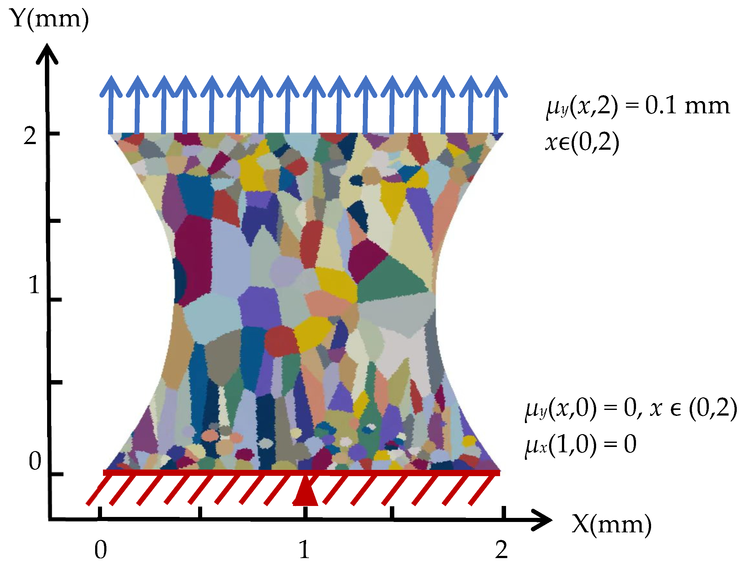
In this CPFE model, displacement boundary conditions are specified as follows: the nodes along the lower boundary of the specimen (y = 0 mm) are fixed in the y-direction translational degree of freedom (DOF 1) to prevent rigid body translation. To further eliminate rigid body drift and enhance computational stability, a single node at the center of the bottom edge (y = 0 mm, x = 1 mm) is additionally constrained in the x-direction (DOF 2). The top region of the specimen (y = 2 mm) is defined as the loading zone, where a constant displacement load of 0.1 mm is applied in the y-direction to achieve uniaxial tensile loading along the y-axis, as illustrated in Figure 2, which shows the uniaxial tensile boundary condition setup.

Figure 2. Uniaxial Tensile Boundary Condition Setup.

The proposed CPC model is applied to finite element models with different grain size gradients. The remaining simulation parameters are listed in Table 1, all parameters listed in Table 1 are adopted from Ref. [33], where their determination and calibration procedures are described in detail.

Table 1. Simulation Parameters.

Property	Value/Range	Unit
C11	168.4	GPa
C12	121.4	GPa
C44	75.4	GPa
$\dot{{\gamma }_0}$	0.001	s−1
n	10	/
q	1	/
h0	800	MPa
k1	[200, 500]	MPa
k2	[20, 60]	MPa
k3	[5, 15]	MPa

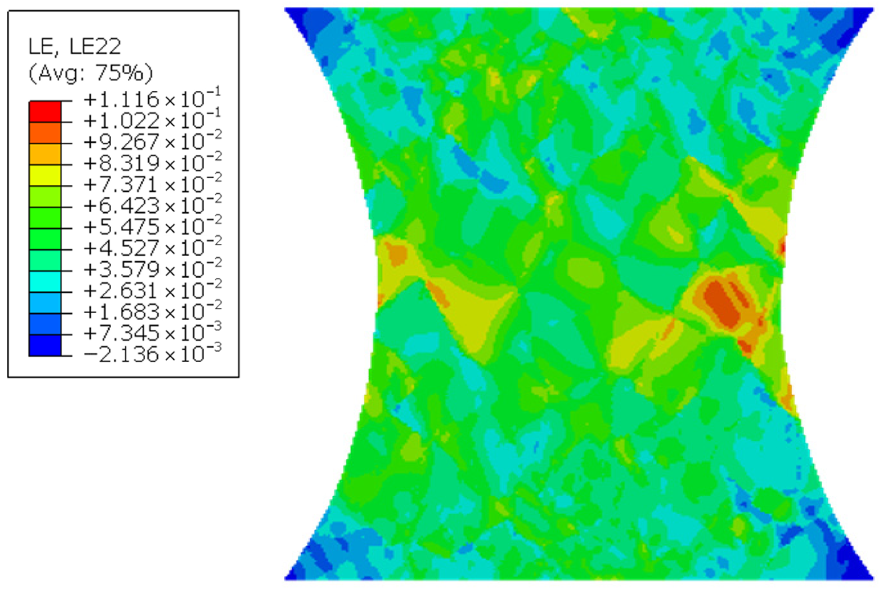
According to the ABAQUS simulation results (as shown in Figure 3), distinct strain response characteristics are observed in regions with different grain sizes. In the central region, which consists of large equiaxed grains, both the yield strength and hardening modulus are relatively low. As a result, plastic flow is initiated at lower stress levels, and substantial plastic strain continues to accumulate throughout subsequent deformation, manifesting as significant strain concentration zones (yellow to red regions). In contrast, the small equiaxed grain regions at both the top and bottom exhibit a high grain boundary density, which substantially increases yield strength and hardening modulus. This allows the material to more effectively resist further plastic deformation after yielding, leading to overall lower and more uniformly distributed strain (blue-green regions). The columnar grain regions, located between the large and small equiaxed grain zones, have moderate grain sizes but, due to their orientation along the long axis, are prone to the formation of slip channels that reduce barriers to dislocation motion, resulting in pronounced local strain elevation.

Figure 3. Strain Simulation Results.

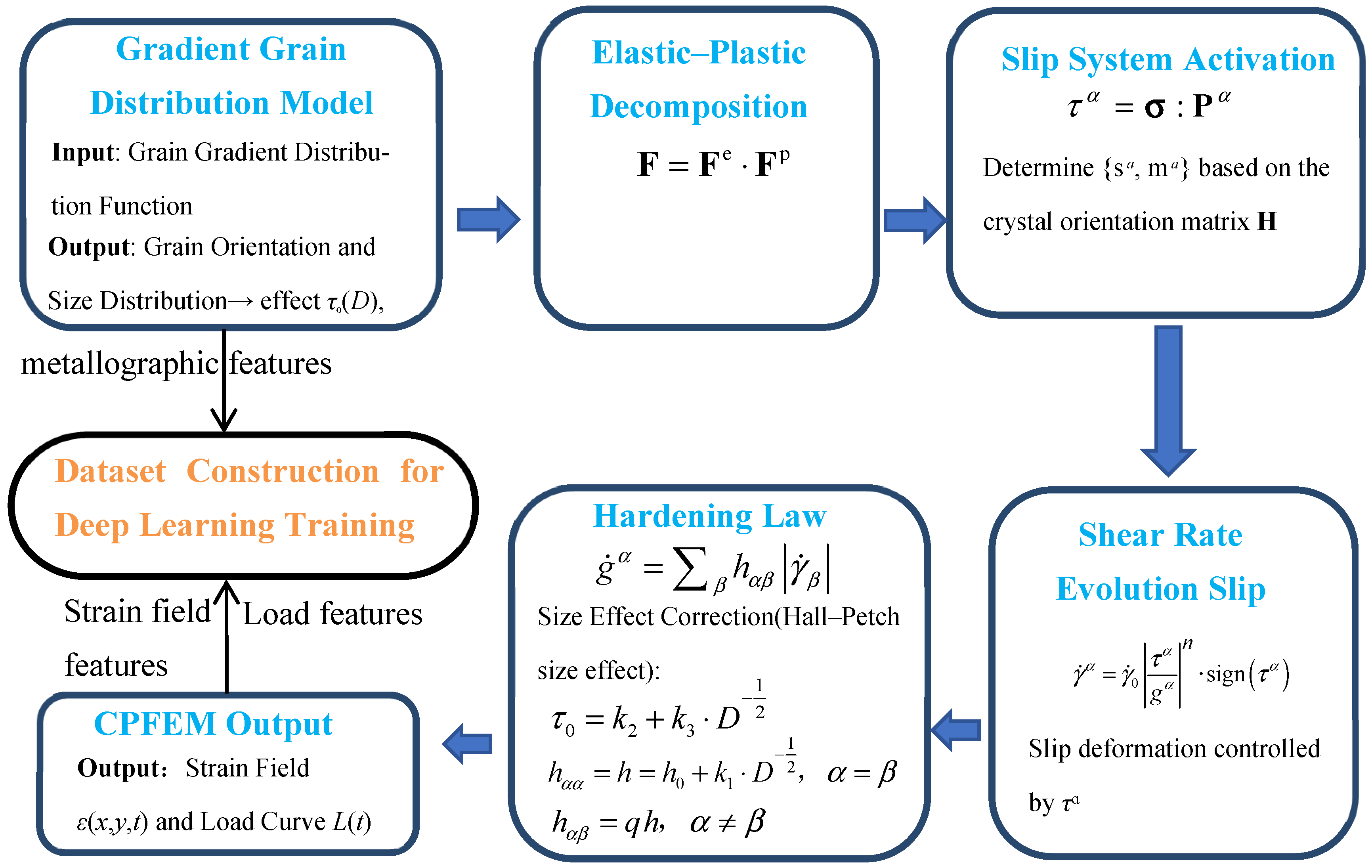
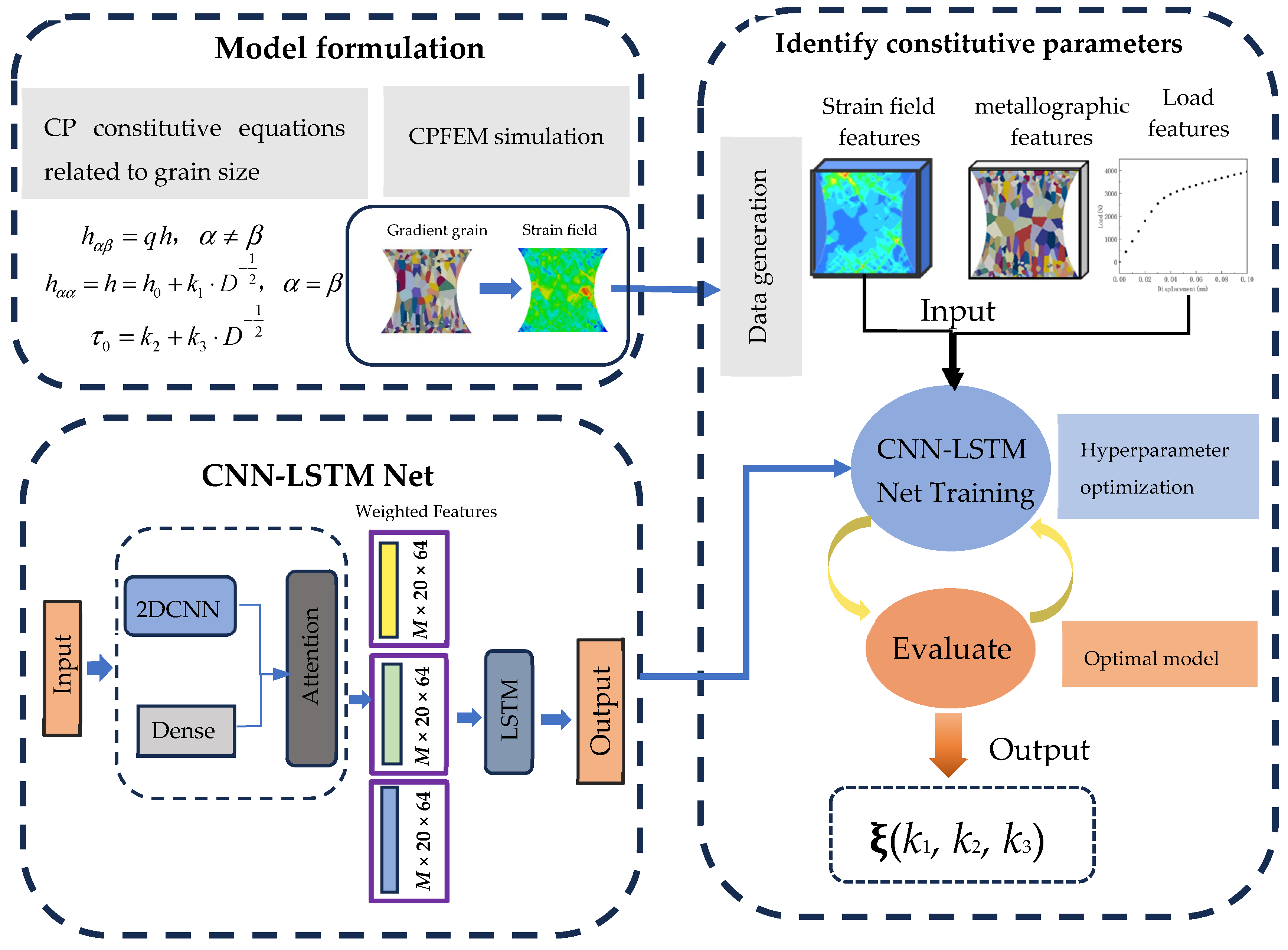
Overall, as grain size increases, both yield strength and hardening modulus decrease, making large-grain regions more susceptible to strain localization under loading, while fine-grained regions effectively disperse plastic deformation by enhancing yield strength and hardening capacity. This pattern not only validates the classic relationship between grain size and plastic deformation behavior but also provides an important basis for the microstructural optimization of weld joints. Figure 4 illustrates the workflow of the gradient-grained CPFEM and dataset construction for deep learning inversion.

Figure 4. Workflow of the gradient-grained CPFEM and dataset construction for deep learning inversion.

3. Deep Learning-Based Parameter Inversion Framework

3.1. Data Generation and Preprocessing

To construct a constitutive parameter inversion model with spatiotemporal resolution, this study first establishes a dataset based on the previously proposed CPFE method. A finite element model with a gradient-grained structure is used in combination with the crystal plasticity constitutive equations to simulate the evolution of strain fields, outputting a sequence of 20 strain field images as time-series input features. Simultaneously, the CPC model (Crystal Plasticity-Cellular model) is employed to simulate grain structures, obtaining grain size and orientation angle information, with the Euler angle distributions statistically characterized to represent the metallographic features of the grains. The simulation process, a Maximin LHS [34] design with a fixed random seed (2025) was adopted to uniformly and non-redundantly sample the parameter space $\mathsf{\xi }$ = (k₁, k₂, k₃), thereby ensuring the reproducibility of the generated dataset.

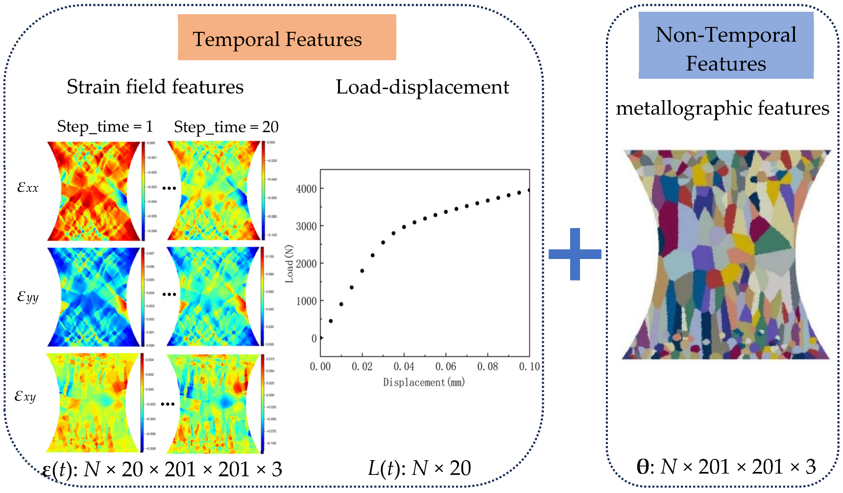
Figure 5 illustrates the composition of the dataset, where N denotes the total number of samples. The input for each sample consists of the following three components:

Figure 5. Composition of the Dataset.

(1)

Temporal strain field sequences: Since the strain field is a time series, a total of 20 time steps are extracted. For each time step, the data for ε_xx, ε_yy and ε_xy in three directions are collected as three separate channels. Each strain field in a given direction is stored as an image of size 201 × 201. The resulting temporal strain field sequence is represented as ε(t) ∈ R_{201×201×3×20}.

(2)

Metallographic structural information: The grain distribution information is non-sequential data and does not include a temporal dimension. For each grain, the three orientation angles correspond to three separate channels, with each orientation angle map represented as an image of size 201 × 201. The resulting grain orientation distribution map (using orientation angles in place of morphological statistics) is given by θ ∈ R_201×201×3.

(3)

Loading sequence: The loading information is time-series data. A total of 20 time steps are extracted, with each time step containing a single scalar load value. The resulting loading sequence is denoted as L(t) ∈ R₂₀.

In this study, a total of 20,000 training samples and 2000 validation samples were generated for training and evaluating the predictive performance of the neural network model.

In terms of data preprocessing, the objective is to enhance data reading efficiency while addressing the storage and computational demands of large-scale sample training. This can be achieved by adopting efficient data serialization formats that support compression and sequential access, thereby reducing I/O latency and improving loading performance. Furthermore, utilizing data pipeline mechanisms enables streaming data processing during model training, which helps balance computational efficiency and memory utilization. Dynamically computing statistical measures of features (e.g., global mean and standard deviation) for normalization further improves the robustness of feature scaling without the need to preload the entire dataset into memory.

Due to the differences in dimensionality and magnitude among the raw input data, standardized preprocessing was applied to improve the training efficiency and convergence stability of the neural network model. Specifically, the input features—including strain field sequences, loading information, and metallographic parameters—were each standardized using the Z-score normalization method, transforming them to zero mean and unit variance. The calculation is given by:

$${\widehat{x}}_j={\displaystyle \frac{x_j-\mu }{\sigma }}$$

(17)

where x_j denotes the j-th raw input feature, while μ and σ represent the global mean and standard deviation of that feature over the training set, respectively. During the training phase, these statistical parameters are dynamically computed and saved to enable reuse for standardizing the test data during the evaluation phase. This approach ensures consistency in data distribution between the training and testing sets and avoids bias that could be introduced by redundant calculations.

For the output labels, namely the constitutive parameter vector ξ, a linear MinMax normalization method is used to map the values to the range [0.1, 1]. To avoid zero-gradient regions of activation functions and to ensure stable gradient propagation, all input features were normalized to the range [0.1, 1] instead of [0, 1], following the normalization approach used in CPINet [16]. The transformation is given by:

$$y_j={\displaystyle \frac{{\xi }_j-{\xi }_j^{\min }}{{\xi }_j^{\max }-{\xi }_j^{\min }}}\cdot \left(y^{\max }-y^{\min }\right)+y^{\min }$$

(18)

where ξ_j denotes the original value of the j-th constitutive parameter, while ${\xi }_j^{\max }$ and ${\xi }_j^{\min }$ are the maximum and minimum values of the j-th parameter in the training set, respectively. y_j is the normalized label for the j-th constitutive parameter, with y^min and y^max set to 0.1 and 1, respectively. This normalization strategy helps prevent gradient vanishing problems caused by inconsistent units or magnitude differences among outputs, thereby ensuring effective backpropagation during the early stages of model training.

During the model prediction phase, the normalized labels are restored to their actual physical parameter ranges using the following denormalization formula:

$${\xi }_j={\displaystyle \frac{y_j-y_j^{\min }}{y_j^{\max }-y_j^{\min }}}\cdot \left({\xi }^{\max }-{\xi }^{\min }\right)+{\xi }^{\min }$$

(19)

3.2. CNN-LSTM Network Architecture Design

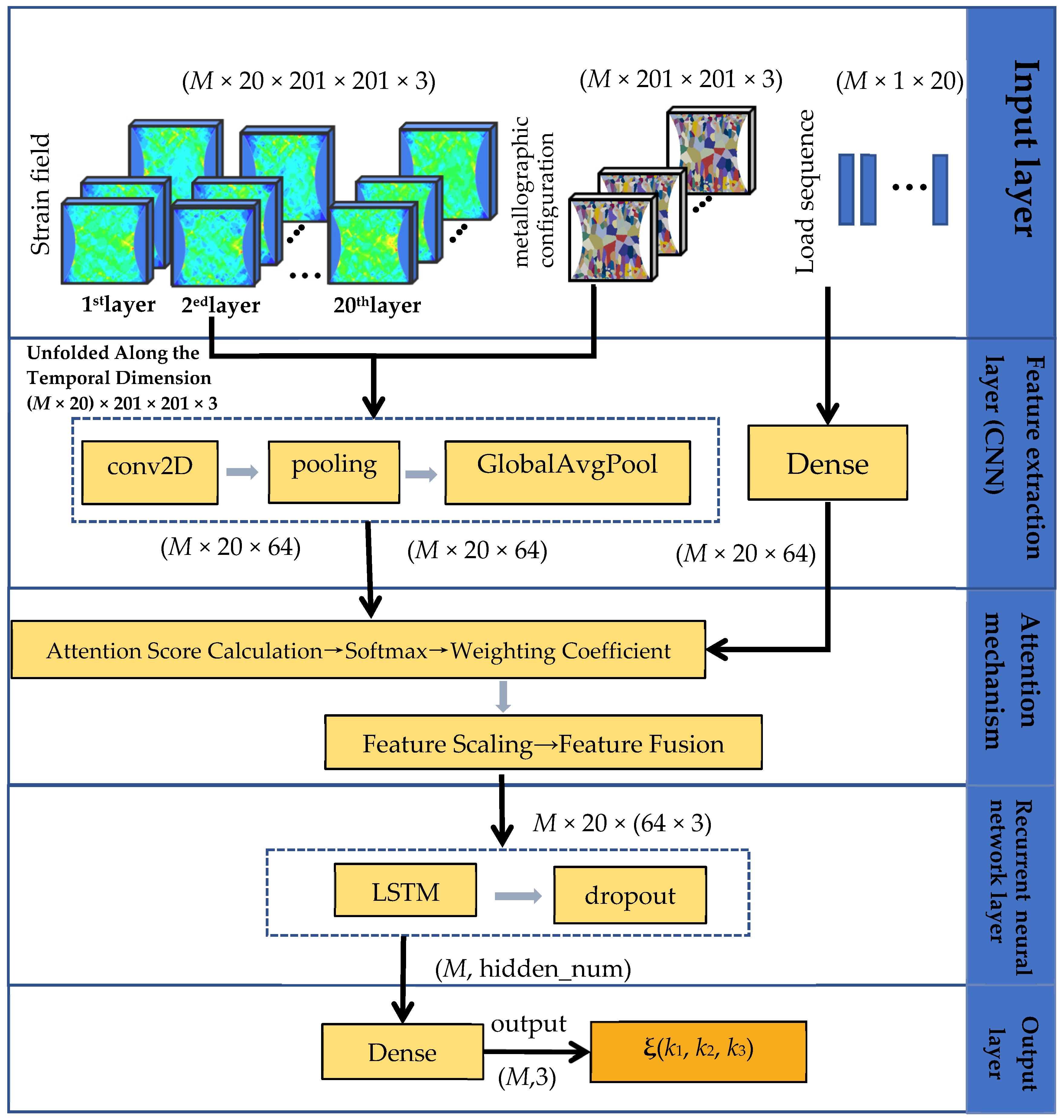
The CNN-LSTM deep neural network model constructed in this study consists of two key components: a CNN module for spatial feature extraction, and a LSTM module for temporal sequence modeling. This architecture is designed to integrate spatial–temporal features present during material deformation, thereby enabling accurate identification of path-dependent constitutive parameters. The structural diagram of this architecture is shown in Figure 6.

Figure 6. Schematic Diagram of the Network Architecture.

3.2.1. CNN Module: Spatial Feature Extraction of Strain Fields and Metallographic Morphology

For ease of storage, all sample data were converted into a one-dimensional format and saved in TFRecord format before being fed into the network. For the input strain field sequences, the data were first reconstructed into a five-dimensional tensor structure (batch_size × step_time, height, width, channel) according to the order in which the data were written. Next, a Permute operation was applied to swap the spatial and channel dimensions, reconstructing the data into (batch_size × step_time, height, width, channel), which is compatible with the input format of the convolutional layers. To enable a shared convolutional kernel extraction strategy across time steps, the temporal dimension was flattened into the batch dimension, effectively “merging” the multiple time frames of each sample into the batch. This transforms the originally sequential data into a unified two-dimensional spatial structure, which is then input into the two-dimensional convolutional network. The operation is illustrated in Figure 7.

Figure 7. Schematic Diagram of Strain Field Feature Reshaping.

Compared with three-dimensional convolution (Conv3D), this strategy significantly reduces the model parameter scale and computational complexity. Conv3D requires the convolutional kernel to slide simultaneously across temporal and spatial dimensions, which enables the capture of spatiotemporal coupled features, but incurs a high computational cost and imposes stricter requirements on data volume. In contrast, by merging the temporal dimension into the batch, two-dimensional convolution (Conv2D) independently extracts spatial features at each time step. The subsequent recurrent neural network (LSTM) then models the temporal dependencies, enabling structural decoupling and optimization. This approach is more flexible and offers superior scalability.

During the convolutional feature extraction process, the sequence images are sequentially passed through four layers of two-dimensional convolutional modules. Each layer consists of a convolutional layer, batch normalization, and a ReLU activation function, with kernel sizes of 5 × 5 and 3 × 3, and output channels set to 16, 32, 64, and 128, respectively. Except for the final layer, max pooling operations are nested within the other layers to compress the spatial feature dimensions, reduce computational load, and enhance the abstraction capacity of the extracted features.

Finally, a Global Average Pooling layer and a fully connected (Dense) layer are applied to map the convolved features into the final output space. The resulting feature shape is (batch_size, step_time, 64).

Simultaneously, the metallographic morphology features (i.e., grain orientation maps) are also input into a separate set of CNN modules. As these metallographic features are four-dimensional tensors (batch_size, height, width, channel), lacking the temporal dimension present in the strain field sequences, only a Permute operation is required to swap the spatial and channel dimensions, reconstructing the data into structure (batch_size × height × width × channel) before being directly input into the Conv2D layers. The same network architecture as that used for the strain fields is employed for static image feature extraction. Since the metallographic structure does not evolve with loading over time, the extracted 64-dimensional feature vector is replicated along the temporal axis to form a time series with a length of 20, in order to concatenate it with the strain field features for joint input into the LSTM network. Thus, the output shape is also (batch_size, step_time, 64), enabling synchronous input into the temporal model together with the strain field features.

When loading features are input into the network, they have the shape (batch_size, step_time, 1). Since the loading feature for each sample consists of relatively few data points, convolutional layers are not necessary for primary feature extraction. Instead, the loading data are passed directly through a Dense layer, transforming the data shape to (batch_size, step_time, 64) which facilitates subsequent concatenation with the other two feature sets for further processing.

3.2.2. Attention Mechanism Module

To further enhance the model’s ability to focus on and dynamically adjust the importance of the three types of features, this study incorporates an attention mechanism, drawing on the classical sequence attention approach of Bahdanau et al. [35] and the self-attention mechanism introduced by Vaswani et al. [36]. By applying attention weighting across the concatenated strain field features, metallographic morphology features, and loading features (batch_size, step_time, 64 × 3) at each time step, the model can autonomously assign greater weight to the most salient features at different time points.

Specifically, the attention mechanism is implemented through the following process: First, the time series inputs of the strain field, metallographic morphology, and loading features are each processed independently. At each time step, an independent fully connected layer computes an attention score for each input feature. These scores reflect the importance of each feature at different time steps. Subsequently, the attention scores are transformed into temporal weights (attention weights) for each feature using a Softmax activation function, ensuring that the sum of the weights at each time step is equal to one. Finally, the attention weights are multiplied elementwise with their corresponding input features to yield the weighted feature representations.

The attention mechanism can be formally represented by the following equations:

For each feature i ∈ {strain, metallographic, load}, the attention score is calculated as follows:

$$S_{i,t}={\mathbf{W}}_i\cdot {\mathbf{X}}_{i,t}+b_i$$

(20)

where S_i,t is the score of feature i at time step t, W_i is the weight matrix for feature i, X_i,t is the input of feature i at time step t, and b_i is the bias term.

For each feature i, the weight at time step t is calculated using the Softmax function:

$${\alpha }_{i,t}={\displaystyle \frac{{\mathrm{e}}^{{\mathbf{s}}_{i,t}}}{{\displaystyle {\sum }_{i\in \left\{\mathrm{s}\mathrm{t}\mathrm{r}\mathrm{a}\mathrm{i}\mathrm{n},\mathrm{g}\mathrm{e}\mathrm{o},\mathrm{l}\mathrm{o}\mathrm{a}\mathrm{d}\right\}}{e}^{S_{i,t}}}}}$$

(21)

where α_i,t denotes the attention weight of feature i at time step t. The denominator is the sum of exponentials of all feature scores, ensuring that the weights at each time step sum to one.

For each feature i, the weighted feature is calculated by element-wise multiplication as follows:

$${\tilde{\mathbf{X}}}_{i,t}={\alpha }_{i,t}\odot {\mathbf{X}}_{i,t}$$

(22)

where ${\tilde{\mathit{X}}}_{i,t}$ denotes the weighted feature, and $\odot$ represents element-wise multiplication.

All weighted features are then concatenated to obtain the final weighted input feature:

$${\tilde{\mathbf{X}}}_t=\left[{\tilde{\mathbf{X}}}_{\mathrm{s}\mathrm{t}\mathrm{r}\mathrm{a}\mathrm{i}\mathrm{n},t},{\tilde{\mathbf{X}}}_{\mathrm{met},t},{\tilde{\mathbf{X}}}_{\mathrm{l}\mathrm{o}\mathrm{a}\mathrm{d},t}\right]$$

(23)

Finally, these weighted features are fed into the temporal model for subsequent modeling. This attention mechanism enables the model to more effectively capture the relationships among different input features and to adaptively adjust the importance of each feature in temporal modeling according to the specific context at each time step. Through this dynamic weighting approach, the model avoids excessive dominance of any single feature over the output, thereby enhancing both its generalization capability and prediction accuracy. Especially in time series tasks, the model can flexibly adjust feature weights at each time step, focusing on the most relevant information and thus improving performance on the prediction task.

3.2.3. LSTM Module: Temporal Modeling of Loading History and Evolution Path

The LSTM network, as a type of recurrent neural network (RNN) with gating mechanisms, is highly effective at capturing temporal dependencies in long sequences and is particularly suited for handling long-term dependency problems. During multi-step loading processes, the current mechanical state of a material is not only directly related to the present strain but is also strongly influenced by the historical evolution of the loading path—that is, the material’s “memory” of prior loading steps, which is a typical example of path dependency. The LSTM network is well suited to such temporally dependent tasks, as its sophisticated gating mechanisms allow for the efficient propagation, retention, and selective forgetting of historical information during sequential computation. This enables the model to capture the cumulative influence of the loading path on the current material state.

The design of the LSTM enables the network to automatically learn important historical information from input features such as load and strain field at different time steps when processing the loading history of materials, and to transmit this information to subsequent time steps as needed. To further exploit the path-dependent characteristics of material deformation, a stacked three-layer LSTM architecture is employed for temporal modeling. The input to the LSTM is a time series vector resulting from the fusion of strain field, metallographic structure, and loading features, with dimensions of (batch_size × time × 192). Each LSTM layer contains 16 neurons, uses the tanh activation function, and incorporates a Dropout layer (dropout rate of 0.3) after each layer to enhance generalization capability. The final output features are mapped to the target constitutive parameter space ξ(k₁, k₂, k₃) (three continuous variables) via a fully connected layer.

The following illustrates the specific process by which the historical features, such as strain, are propagated through the LSTM network along the time sequence.

The input gate i_t regulates the influence of the current input x_t (i.e., the attention-weighted strain field, metallographic, and loading features) on the memory cell state. By performing a weighted sum of the current input and the previous hidden state, the input gate determines which new information is to be incorporated into the memory cell. At this stage, information from each moment in the strain history is integrated into the memory cell state h_t−1,

$${\mathbf{i}}_t=\phi \left({\mathbf{W}}_i\cdot \left[{\mathbf{h}}_{t-1},{\mathbf{x}}_t\right]+{\mathbf{b}}_i\right)$$

(24)

where W_i is the weight matrix, b_i is the bias term, and φ denotes the Sigmoid activation function. The output values range between [0, 1], representing the proportion of information retained.

The forget gate f_t regulates how much information from the previous memory cell state C_t−1 is retained in the current memory cell state. During the evolution of strain fields and loading, some historical information may become irrelevant; the forget gate enables the selective discarding of such information.

$${\mathbf{f}}_t=\phi \left({\mathbf{W}}_{\mathbf{f}}\cdot \left[{\mathbf{h}}_{t-1},{\mathbf{x}}_t\right]+{\mathbf{b}}_f\right)$$

(25)

The candidate memory cell state ${\tilde{\mathit{C}}}_t$ at the current time step is computed from the current input and the previous hidden state. It determines which new information from the strain history should be incorporated into the memory cell, thereby further influencing the material’s future response.

$${\tilde{\mathit{C}}}_t=\tanh \left({\mathbf{W}}_i\cdot \left[{\mathbf{h}}_{t-1},{\mathbf{x}}_t\right]+{\mathbf{b}}_i\right)$$

(26)

where tanh denotes the hyperbolic tangent activation function, which constrains the candidate memory values within the range [−1, 1].

The updated memory cell state C_t is a weighted sum of the previous memory and the current candidate memory. The forget gate and input gate together determine the retention and updating of strain history. As a result, the memory cell state not only contains the current strain information but also integrates the influence of prior history.

$${\mathit{C}}_t={\mathbf{f}}_t\odot {\mathit{C}}_{t-1}+{\mathbf{i}}_t\odot {\tilde{\mathit{C}}}_t$$

(27)

The output gate o_t controls the final hidden state h_t, which is the network’s output. The hidden state output is a compressed representation extracted from the current memory cell state C_t, and is passed to downstream network layers or used for prediction.

$${\mathbf{o}}_t=\sigma \left({\mathbf{W}}_o\cdot \left[{\mathbf{h}}_{t-1},{\mathbf{x}}_t\right]+{\mathbf{b}}_o\right)$$

(28)

Finally, the current hidden state ${\mathit{h}}_t$ is computed as follows:

$${\mathbf{h}}_t={\mathbf{o}}_t\odot \tanh \left({\mathit{C}}_t\right)$$

(29)

Through the aforementioned gating mechanisms, the LSTM is able to efficiently handle long-term dependency problems, retaining important information while discarding irrelevant data, thereby capturing the evolutionary influence of the loading path on the current material strain state. By integrating the LSTM network with the previously described CNN and attention mechanism modules, the proposed model can efficiently process strain field, metallographic, and loading features in both spatial and temporal dimensions, capturing their interactions and evolutionary patterns. The complete network architecture is illustrated in Figure 8.

Figure 8. CNN-LSTM Net Network Architecture Diagram.

By comparing the prediction efficiency, accuracy, and noise robustness of the network under different structural parameters, the optimal configuration of the Net is determined, as summarized in Table 2.

Table 2. Network Structural Parameters.

Feature Category	Layer Name	Kernel Size	Stride	Operator	Number or Method	Padding	Activation Function	Dropout
Geometry/strain Features	Conv1	5 × 5	(1, 1)	Conv2D	Filters 16	Same	ReLU	-
Geometry/strain Features	Pool1	2 × 2	(2, 2)	MaxPooling2D	-	Valid	-	-
Geometry/strain Features	Conv2	5 × 5	(1, 1)	Conv2D	Filters 32	Same	ReLU	-
Geometry/strain Features	Pool2	2 × 2	(2, 2)	MaxPooling2D	-	Valid	-	-
Geometry/strain Features	Conv3	3 × 3	(1, 1)	Conv2D	Filters 64	Same	ReLU	-
Geometry/strain Features	Pool3	2 × 2	(2, 2)	MaxPooling2D	-	Valid	-	-
Geometry/strain Features	Conv4	3 × 3	(1, 1)	Conv2D	Filters 128	Same	ReLU	-
Load Features	FC Layer1	-	-	Dense	Number 64	-	ReLU	-
Geometry/Strain/Load Features	Attention1 (Score)	-	-	Dense×2	Number 32/1	-	tanh/linear	-
Geometry/Strain/Load Features	Attention2 (Apply)	-	-	Softmax → Multiply	-	-	Softmax	-
Weighted Features	LSTM	-	-	LSTM	Hidden 128	-	tanh	0.3
Output Features	FC Layer2	-	-	Dense	Neurons 3	-	-	-

3.3. Training Configuration and Optimization

During model training, the appropriate selection of loss functions, optimizer settings, learning rate scheduling strategies, and validation metrics is crucial for enhancing both training effectiveness and generalization capability. The following provides a detailed description of the configurations and optimization strategies employed in this study.

3.3.1. Loss Function

To quantitatively assess the predictive performance of the proposed model and appropriately measure the deviation between predicted and true values, this study employs Mean Squared Error (MSE) and Mean Absolute Error (MAE) as the loss functions and evaluation metrics in the normalized feature space. Specifically, MSE effectively amplifies larger deviations and is suitable for measuring overall fitting error, while MAE is less sensitive to outliers and better reflects the robustness of the predictions. Their mathematical definitions are as follows.

Mean Squared Error (MSE) calculates the average of the squared differences between normalized predicted values and true values across all samples, and is defined as:

$$\mathrm{M}\mathrm{S}\mathrm{E}\left(y_{\mathrm{true}},y_{\mathrm{pred}}\right)={\displaystyle \frac{1}{N}}{\displaystyle {\sum }_{i=1}^N{\left(y_{\mathrm{true}}^{\left(i\right)}-y_{\mathrm{pred}}^{\left(i\right)}\right)}^2}$$

(30)

Mean Absolute Error (MSE) calculates the average of the absolute differences between normalized predicted values and true values across all samples, and is defined as:

$$\mathrm{M}\mathrm{A}\mathrm{E}\left(y_{\mathrm{true}},y_{\mathrm{pred}}\right)={\displaystyle \frac{1}{N}}{\displaystyle {\sum }_{i=1}^N\left|y_{\mathrm{true}}^{\left(i\right)}-y_{\mathrm{pred}}^{\left(i\right)}\right|}$$

(31)

where N denotes the total number of samples, while ${\mathrm{y}}_{\mathit{true}}^{\left(i\right)}$ and ${\mathrm{y}}_{\mathit{pred}}^{\left(i\right)}$ represent the normalized true value and predicted value of the i-th sample, respectively.

Relying solely on loss functions often fails to comprehensively reflect a model’s performance from multiple perspectives. Therefore, in both the training and validation phases, this study uses MSE and MAE as the primary loss metrics, while additionally incorporating the coefficient of determination (R²) and training computational time as supplementary evaluation criteria. This allows for a comprehensive assessment of the model’s predictive accuracy and computational efficiency.

The coefficient of determination R² measures the goodness of fit between the predicted results and the true data, and is defined as:

$$R^2=1-{\displaystyle \frac{{{\displaystyle \sum \left(y_{\mathrm{true}}^{(i)}-y_{\mathrm{pred}}^{(i)}\right)}}^2}{{{\displaystyle \sum \left(y_{\mathrm{true}}-{\overline{y}}_{(i)}\right)}}^2}}$$

(32)

where ${\overline{y}}_{\left(i\right)}$ represents the i-th mean of the true values. The closer the R² value is to 1, the better the model’s fit.

It should be noted that all predicted and true values are normalized using the global mean μ and standard deviation σ determined during the training phase, ensuring consistency in data distribution between the training and testing stages.

3.3.2. Optimizer

In the training of deep neural networks, the choice of optimizer directly impacts the efficiency of parameter updates and the overall convergence speed of the model. To address potential issues such as training oscillations, slow convergence, and gradient vanishing, this study employs the Adaptive Moment Estimation (Adam) optimizer [37], which has been widely validated in deep learning for its effectiveness. Adam leverages adaptive learning rates and momentum, making it particularly advantageous for handling non-stationary objectives and sparse gradients.

Adam combines the concepts of RMSProp and Momentum by simultaneously maintaining first-order moments (momentum) and second-order moments (adaptive variance) during gradient updates. This significantly mitigates the instability often encountered in traditional optimization algorithms, thereby effectively enhancing training efficiency and robustness. The parameter update formula can be expressed as follows:

$${\theta }_t={\theta }_{t-1}-{\displaystyle \frac{\eta }{\sqrt{v_t}+\delta }}{m}_t$$

(33)

where θ_t represents the network parameters at the current iteration, m_t and v_t are the first- and second-moment estimates of the gradients, respectively, $\mathsf{\eta }$ denotes the learning rate, and δ is a small constant added to prevent division by zero.

3.3.3. Repeated 10-Fold Cross-Validation

To further evaluate the model’s sensitivity and stability with respect to the partitioning of validation samples, a repeated 10-fold cross-validation was conducted. In each repetition, the validation dataset was randomly divided into ten subsets, with one subset used as the validation set and the remaining nine subsets used for training and evaluation. This process was repeated for 20 rounds with different random seeds, resulting in a total of 200 sub-evaluations

In the j-th evaluation (j = 1, …, m, where m = 200), the validation sample set is denoted as D_j with a sample size of N_j. The three performance metrics on this fold—MAE_j, RMSE_j, and R_j²—were computed as follows:

$$MA{E}_j={\displaystyle \frac{1}{N_j}}{\displaystyle \sum _{i\in D_j}\left|y_{i,j}-{\widehat{y}}_{i,j}\right|}$$

(34)

$$RMS{E}_j=\sqrt{{\displaystyle \frac{1}{N_j}}{\displaystyle \sum _{i\in D_j}{\left(y_{i,j}-{\widehat{y}}_{i,j}\right)}^2}}$$

(35)

$$R_j^2=1-{\displaystyle \frac{{\displaystyle \sum _{i\in D_j}{\left(y_{i,j}-{\widehat{y}}_{i,j}\right)}^2}}{{\displaystyle \sum _{i\in D_j}{\left(y_{i,j}-{\overline{y}}_j\right)}^2}}}.$$

(36)

Here, $y_{i,j}$, ${\widehat{y}}_{i,j}$ and ${\overline{y}}_j$ represent the denormalized true value, predicted value, and mean of the true values for the i-th sample in the j-th fold, respectively.

Consequently, the results of MAE and RMSE are expressed in the physical unit (MPa). A total of 200 scalar sequences ${\left\{M_j\right\}}_{j=1}^m$ were obtained, where M_j ∈ {MAE_j, RMSE_j, R_j²}. To quantify the stability across different data partitions, statistical aggregation was performed on each sequence as follows. Under random partitioning, the expected performance of each metric is characterized by its mean $m$, standard deviation $s_m$, and 95% confidence interval (CI), which are defined as follows:

$$\overline{M}={\displaystyle \frac{1}{m}}{\displaystyle \sum _{j=1}^m{M}_j}$$

(37)

$$S_M=\sqrt{{\displaystyle \frac{1}{m-1}}{\displaystyle \sum _{j=1}^m{\left(M_j-\overline{M}\right)}^2}}$$

(38)

$$\overline{M}\pm t_{0.975,m-1}{\displaystyle \frac{s_M}{\sqrt{m}}}$$

(39)

where t_0.975,m−1 denotes the 97.5th quantile (critical value) of the t-distribution with m − 1 degrees of freedom.

Based on the above statistical results, the mean, standard deviation, and 95% confidence interval of each performance metric were reported. These statistics were then used to analyze the stability of the model under different random data partitions and the consistency of its fitting capability.

4. Results and Discussion

To achieve the aforementioned objectives, this study adopts a model architecture based on the integration of CNN and LSTM networks. The CNN component is employed to extract latent spatial organizational features from grain images, while the LSTM component captures the temporal evolution patterns of strain sequences. All training data are derived from CPFE simulation results, covering various grain distributions, loading paths, and boundary conditions, thereby ensuring good generalizability of the model. Although this study does not explicitly introduce complex physical consistency constraints—such as constitutive residuals or energy conservation expressions—the constructed end-to-end deep inversion model is trained on high-fidelity CPFE simulation data, which inherently encapsulates key physical mechanisms such as crystal slip, strain hardening, and grain orientation evolution. Therefore, without increasing the modeling complexity, the model is able to learn physically reasonable response mappings to a certain extent.

4.1. Training Results of the CNN-LSTM Model

By comparing the effects of different training hyperparameters (e.g., learning rate and batch size) and CNN structural parameters (e.g., number of CNN layers) on the performance of the CNN-LSTM network for constitutive parameter identification, this study investigates the impact of various hyperparameter settings on model performance and prediction accuracy. The superscript a in the table denotes the optimal hyperparameters. Experimental results demonstrate that an appropriate selection of learning rate, batch size, and the number of CNN layers can significantly enhance the model’s fitting capability and generalization ability.

Table 3 and Table 4, respectively, compare the prediction accuracy (R²) of the CNN-LSTM Net for CPFEM constitutive parameters under different learning rates and batch sizes. The R² metric reflects the degree of fit between the model’s predictions and observed values, with higher values indicating that the model explains more data variance and thus possesses stronger predictive capability. As the learning rate decreases, the model’s performance during training improves progressively. Specifically, models trained with learning rates of 0.01, 0.001, 0.0001 and 0.00001 exhibit a stepwise increase in prediction accuracy, with the best results for k₁, k₂, k₃ and overall error achieved at a learning rate of 0.0001.

Table 3. Prediction Accuracy (R²) of CNN-LSTM Net under Different Learning Rates.

Learning Rate	k1	k2	k3	Overall
0.01	0.955	0.928	0.909	0.930
0.001	0.974	0.960	0.925	0.953
0.0001 a	0.971	0.963	0.937	0.958
0.00001	0.936	0.758	0.491	0.728

The superscript “a” corresponds to the value of the learning rate, representing its value in the parameter combination of the optimal model.

Table 4. Prediction Accuracy (R²) of CNN-LSTM Net under Different Batch Sizes.

Batch Size	k1	k2	k3	Overall
8 a	0.971	0.963	0.937	0.958
16	0.958	0.942	0.902	0.933
32	0.972	0.965	0.931	0.955

The superscript “a” corresponds to the value of the batch size, representing its value in the parameter combination of the optimal model.

Additionally, the tables illustrate the impact of different batch sizes on model performance, showing that a batch size of 8 yields the best results. It is important to note that varying training parameters also affects the overall training process, leading to different optimal network parameter combinations. For example, when the learning rate is set to 0.0001, more iterations are required to update the weight parameters effectively.

Table 5 compares the fitting performance of the CNN-LSTM Net for constitutive parameters trained with different numbers of CNN layers. It is observed that fitting accuracy varies to some extent, with the four-layer CNN configuration demonstrating superior feature extraction capability. This improvement is attributed to the increased filter depth, which enables the CNN to extract more refined and abstract features from the input data. Consequently, the network can more effectively focus on salient features while reducing redundancy in the input. Despite variations in training parameters, the consistent model architecture ensures that the final CNN-LSTM Net exhibits strong feature extraction ability and prediction accuracy. Based on this analysis, the optimal hyperparameters are determined as follows: learning rate of 0.0001, batch size of 8, and 4 CNN layers.

Table 5. Prediction Accuracy (R²) of CNN-LSTM Net with Different Numbers.

Number of Layers	k1	k2	k3	Overall
2	0.959	0.952	0.926	0.942
3	0.964	0.957	0.925	0.949
4 a	0.971	0.963	0.937	0.958

The superscript “a” corresponds to the value of the number of layers, representing its value in the parameter combination of the optimal model.

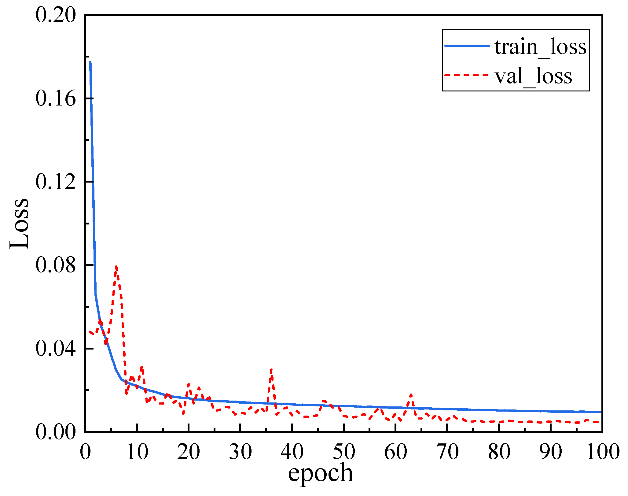
The CNN-LSTM network was constructed and trained based on TensorFlow. Prior to training, the parameter weights were randomly initialized following a normal distribution N(0,1). Figure 9 illustrates the variation trends of the loss function for the training and validation sets during the training process. As shown in the figure, the training loss decreases rapidly in the early stages, indicating that the model effectively captures the fundamental mapping relationships among the samples in a short period of time. In contrast, the validation loss exhibits more pronounced oscillations in the initial stage, primarily due to the relatively large learning rate and the instability of the moving averages of the mean and variance at the beginning, which lead to substantial fluctuations in the model’s responses across different batches. Nevertheless, the overall trend demonstrates a continued decline.

Figure 9. Training and Validation Loss During the Training Process.

As training progresses, the moving averages gradually converge, and, influenced by the piecewise constant decay strategy, the learning rate decreases step by step. This leads to a steady improvement in the model’s generalization performance on the validation set. Ultimately, at the 95th epoch, the validation loss reaches its minimum, with the training and validation losses recorded at 0.0096 and 0.0044, respectively, and the MAE values at 0.0731 and 0.0473. These results indicate that the model has essentially converged and possesses strong generalization capability. Therefore, the CNN-LSTM Net corresponding to this training epoch is selected as the optimal model for subsequent prediction tasks.

4.2. Prediction Results of the CNN-LSTM Model

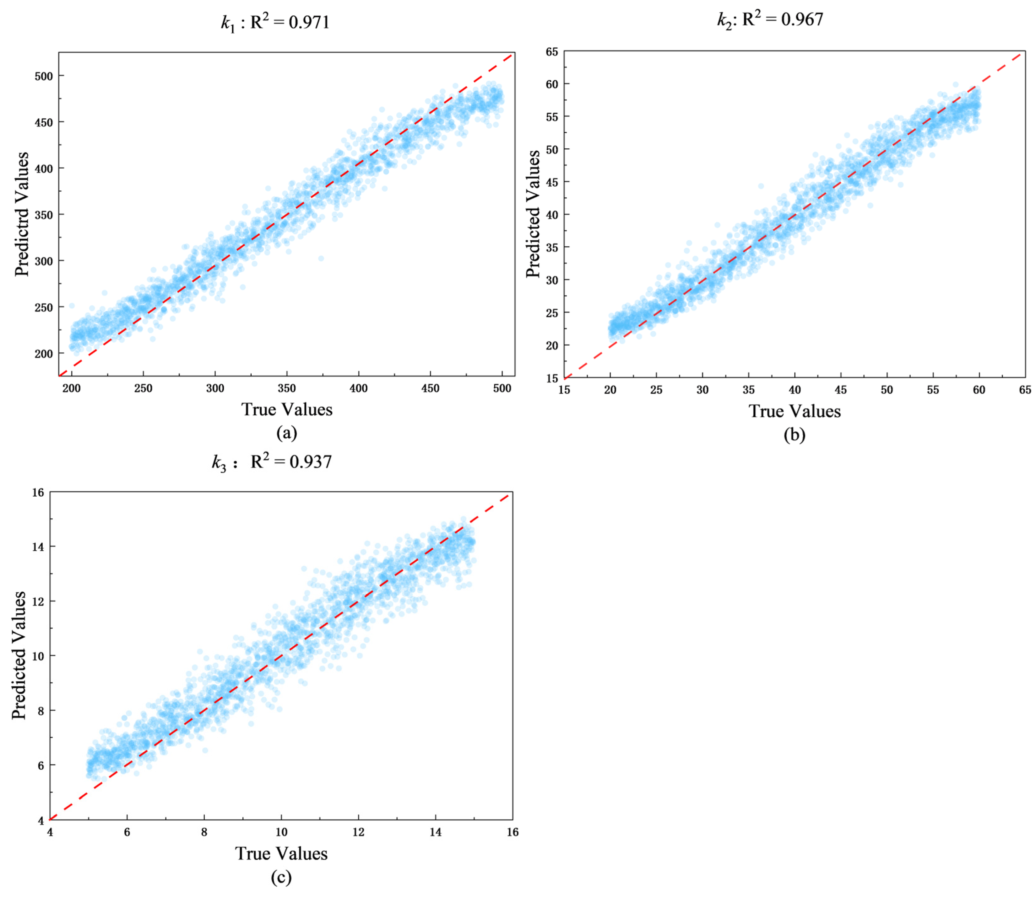
The prediction results obtained using the optimal model (trained with the designed network architecture) are as follows: the prediction accuracies for the three parameters k₁, k₂ and k₃ are 0.971, 0.967, and 0.937, respectively, while the overall prediction accuracy of the constitutive parameters is 0.958. The prediction error is less than 5%, indicating that the developed deep learning model can accurately invert the crystal plasticity constitutive parameters. To provide a more intuitive validation, Figure 10 presents the correlation plots between the predicted and true values of the three parameters, including all 2000 sample points from the training dataset. The data points are closely distributed along the diagonal line, confirming the strong consistency between predictions and ground truth.

Figure 10. Correlation between predicted and true values of the constitutive parameters k₁, k₂, and k₃. Panels (a–c) show the correlation for k₁, k₂, and k₃, respectively.

Figure 11 illustrates the distribution of attention weights for three feature types—strain, geometry, and load—at different time steps for Sample 1. The green, orange, and blue curves correspond to the attention weights of strain, geometry, and load features, respectively. It can be observed that the strain features consistently maintain the highest attention weight and gradually stabilize as deformation proceeds, indicating that the temporal evolution of strain fields provides the most critical information for constitutive parameter identification. The geometry-related features exhibit a moderate increase at early stages, reflecting the influence of microstructural gradients on local hardening behavior, while the load features rapidly decrease as the time steps progress, suggesting that global loading information becomes less dominant once internal strain localization develops.

Figure 11. Attention Weight Distribution.

Overall, the dynamic variation of attention weights reveals the physical correspondence between feature importance and the deformation process, confirming that the attention mechanism effectively captures the key spatial-temporal dependencies in strain-field evolution and enhances the interpretability of the CNN-LSTM inversion model.

4.3. Model Validation and Stability Analysis

To evaluate the generalization capability of the model, a repeated 10-fold cross-validation procedure was employed to quantitatively assess the prediction performance of the three constitutive parameters k₁, k₂, and k₃, as summarized in Table 6. In this process, the entire dataset, consisting of 22,000 samples, was randomly divided into 10 folds. In each repetition of the cross-validation, 9 folds were used for training, and the remaining 1 fold was used for validation. This procedure was repeated 20 times, resulting in a total of 200 sub-evaluations.

Table 6. Statistical summary of predictive performance metrics of constitutive parameters under 10-fold cross-validation.

Metric	Constitutive Parameters	Mean	Standard Deviation (Std)	95% Confidence Interval (95%CI)	Coefficients of Variation (CV) (%)
MAE	k1	11.425	0.576	[11.344, 11.505]	5.04
	k2	1.717	0.085	[1.705, 1.729]	4.95
	k3	0.576	0.031	[0.572, 0.580]	5.42
RMSE	k1	14.539	0.748	[14.435, 14.644]	5.14
	k2	2.130	0.098	[2.116, 2.143]	4.58
	k3	0.717	0.034	[0.713, 0.722]	4.74
R2	k1	0.970	0.004	[0.970, 0.971]	0.37
	k2	0.969	0.004	[0.966, 0.972]	0.41
	k3	0.937	0.006	[0.936, 0.938]	0.64

The coefficient of determination (R²) values of the three models are all close to 1, indicating excellent goodness of fit and that the models can, respectively, explain approximately 97.0%, 96.9%, and 93.7% of the total variance in the data. Among them, k₁ exhibits the highest R² value, suggesting that the model achieves the most accurate fitting performance for k₁ relative to its intrinsic data variability.

The coefficients of variation (CV = Std/Mean × 100%) for the MAE and RMSE performance metrics of the three constitutive parameters are all below 6%, and the 95% confidence intervals exhibit narrow distributions. This indicates that the model predictions remain highly consistent across multiple random partitions and repeated training runs, demonstrating excellent statistical stability and reliability of the inversion results. Specifically, for parameter k₂, the CV of MAE is 4.95%, which is lower than those of k₁ (5.04%) and k₃ (5.42%). Similarly, the CV of RMSE for k₂ is 4.58%, also lower than that of k₁ (5.14%) and k₃ (4.74%). These results suggest that the inversion of k₂ exhibits higher stability and consistency, with a more concentrated error distribution. This further implies that the network achieves more adequate feature learning and better generalization capability for parameter k₂.

5. Conclusions and Outlook

This study proposes a deep learning inversion framework that integrates CNN and LSTM to efficiently identify key constitutive parameters related to τ₀ and h in gradient-grained structured materials. The model leverages CNN to extract spatial structural features from grain structure images and strain field images, while LSTM captures the temporal evolution patterns of the strain fields and loading conditions during the loading process, thus achieving spatiotemporal coupled modeling under complex multimodal inputs.

(1)

This study extended the crystal plasticity constitutive model to quantify the influence of grain size and orientation on the plastic deformation behavior of gradient-grained FCC metals. The simulation results demonstrated that the model can effectively capture the deformation heterogeneity and strength variation induced by grain-size and orientation gradients, providing a reliable framework for analyzing gradient-grained structures in single-phase FCC alloys.

(2)

The training data for the model were derived from CPFE simulations of gradient-grained distributions, encompassing a variety of grain structure configurations to ensure both representativeness and physical fidelity. Without the explicit incorporation of physical consistency constraints (e.g., residuals or conservation terms), the constructed end-to-end network—built upon high-fidelity CPFE data—was capable of autonomously learning and mapping physically reasonable constitutive parameters related to τ₀ and h₀. Experimental results demonstrated that the prediction accuracies for the three constitutive parameters inverted by the CNN-LSTM Net were 0.971, 0.967, and 0.937, respectively, with the overall prediction error for the three parameters being less than 5%.

(3)

The CNN-LSTM Net demonstrated excellent predictive accuracy and stability across multiple test scenarios. The proposed multimodal deep inversion method not only provides a high-precision, high-efficiency, and physically consistent solution for the identification of crystal plasticity constitutive parameters, but also exhibits broad generalizability, making it applicable to various gradient-grained constitutive models and specimen sizes. The introduction of this approach expands the application boundaries of data-driven methods in microstructure-sensitive materials modeling.

It should be noted that the present framework assumes dislocation slip–dominated plasticity under quasi-static loading and moderate temperature conditions. Effects such as deformation twinning, phase transformation, and high strain-rate responses were not explicitly modeled and will be considered in future extensions [38]. Furthermore, the training dataset was derived from CPFE simulations under idealized gradient morphologies. Future work will incorporate experimental validation, random orientation distributions, and multi-scale data fusion to enhance model generalization and realism.

The proposed CNN-LSTM framework can be effectively applied to the design and optimization of gradient-grained alloys for aerospace structures. By reconstructing spatially varying constitutive parameters, it enables digital-twin-based performance prediction and supports material-by-design strategies in advanced engineering applications. The required strain-field inputs can be obtained through Scanning Electron Microscopy–Digital Image Correlation (SEM–DIC) measurements, which provide microscale full-field strain data consistent with the CPFEM-generated training patterns. In cases where direct strain acquisition is difficult, equivalent strain fields from finite element simulations or localized DIC measurements can also be employed. This flexibility allows the framework to be extended to material characterization, residual stress evaluation, and process optimization of gradient-grained structures.

In future work, the influence of crystallographic orientation distribution will be further considered to enhance the physical completeness of the model. The orientation distribution function (ODF) provides a quantitative link between texture and anisotropic mechanical behavior.

References

1. Zhang, X.; Zhao, J. Geometrically necessary dislocations and related kinematic hardening in gradient grained materials: A nonlocal crystal plasticity study. Int. J. Plast. 2023, 163, 103553. [Google Scholar] [CrossRef]
2. Li, X.; Zhao, J. Revealing the inhibition mechanism of grain size gradient on crack growth in gradient nano-grained materials. Int. J. Solids Struct. 2019, 172–173, 1–9. [Google Scholar] [CrossRef]
3. Shao, J.; Yu, G. Grain size evolution under different cooling rate in laser additive manufacturing of superalloy. Opt. Laser Technol. 2019, 119, 105662. [Google Scholar] [CrossRef]
4. Kan, W.; Chen, B. Formation of columnar lamellar colony grain structure in a high Nb-TiAl alloy by electron beam melting. J. Alloys Compd. 2019, 809, 151673. [Google Scholar] [CrossRef]
5. Wu, X.L.; Jiang, P. Synergetic strengthening by gradient structure. Mater. Res. Lett. 2014, 2, 185–191. [Google Scholar] [CrossRef]
6. Yang, M.; Pan, Y.; Yuan, F.; Zhu, Y.; Wu, X. Back stress strengthening and strain hardening in gradient structure. Mater. Res. Lett. 2016, 4, 145–151. [Google Scholar] [CrossRef]
7. Lin, Y.; Pan, J. Mechanical properties and optimal grain size distribution profile of gradient grained nickel. Acta Mater. 2018, 153, 279–289. [Google Scholar] [CrossRef]
8. Zhao, J.; Lu, X. Constitutive modeling of the tension-compression behavior of gradient structured materials. arXiv 2020, arXiv:2002.03775. [Google Scholar] [CrossRef]
9. Roters, F.; Eisenlohr, P. Overview of constitutive laws, kinematics, homogenization and multiscale methods in crystal plasticity finite-element modeling: Theory, experiments, applications. Acta Mater. 2010, 58, 1152–1211. [Google Scholar] [CrossRef]
10. Sedighiani, K.; Traka, K.; Roters, F.; Sietsma, J.; Raabe, D.; Diehl, M. Crystal plasticity simulation of in-grain microstructural evolution during large deformation of IF-steel. Acta Mater. 2022, 237, 118167. [Google Scholar] [CrossRef]
11. Zheng, X.; Sun, T. Modeling of polycrystalline material microstructure with 3D grain boundary based on Laguerre-Voronoi tessellation. Materials 2022, 15, 1996. [Google Scholar] [CrossRef]
12. Liu, L.-Y.; Yang, Q.-S. Crystal cracking of grain-gradient aluminum by a combined CPFEM-CZM method. Eng. Fract. Mech. 2021, 242, 107507. [Google Scholar] [CrossRef]
13. Herath, C.; Wijesinghe, K. Hierarchical deformation and anisotropic behavior of (α+β) Ti alloys: A micro structure-informed multiscale constitutive model study. Int. J. Plast. 2024, 183, 104163. [Google Scholar] [CrossRef]
14. Hu, Y.; Yu, H. Machine learned mechanical properties prediction of additively manufactured metallic alloys: Progress and challenges. Chin. J. Theor. Appl. Mech. 2024, 56, 1892–1915. [Google Scholar]
15. Zeng, Q.; Zhao, Z. A deep learning approach for inverse design of gradient mechanical metamaterials. Int. J. Mech. Sci. 2023, 240, 107920. [Google Scholar] [CrossRef]
16. Guo, Z.; Bai, R. CPINet: Parameter identification of path-dependent constitutive model with automatic denoising based on CNN-LSTM. Eur. J. Mech. A Solids 2021, 90, 104327. [Google Scholar] [CrossRef]
17. Hu, Y.; Zhou, G. A temporal graph neural network for cross-scale modelling of polycrystals considering microstructure interaction. Int. J. Plast. 2024, 179, 104017. [Google Scholar] [CrossRef]
18. Li, J.; Pokkalla, D.K.; Wang, Z.-P.; Wang, Y. Deep learning-enhanced design for functionally graded auxetic lattices. Eng. Struct. 2023, 292, 116477. [Google Scholar] [CrossRef]
19. Jadoon, A.A.; Kalina, K.A.; Rausch, M.K.; Jones, R.; Fuhg, J.N. Inverse design of anisotropic microstructures using physics-augmented neural networks. J. Mech. Phys. Solids 2025, 203, 106161. [Google Scholar] [CrossRef]
20. Bazyar, M.M.; Tabary, S.A.A.B.; Rahmatabdi, D.; Mohammadi, K.; Hashemi, R. A novel practical method for the production of Functionally Graded Materials by varying exposure time via photo-curing 3D printing. J. Manuf. Process. 2023, 103, 136–143. [Google Scholar] [CrossRef]
21. Hu, Z.; Ma, Z.; Yu, L.; Liu, Y. Functionally graded materials with grain-size gradients and heterogeneous microstructures achieved by additive manufacturing. Scripta Mater. 2023, 226, 115197. [Google Scholar] [CrossRef]
22. Dai, G.; Xue, M.; Guo, Y.; Sun, Z.; Chang, H.; Lu, J.; Li, W.; Panwisawas, C.; Alexandrov, I. Gradient microstructure and strength–ductility synergy improvement of 2319 aluminum alloys by hybrid additive manufacturing. J. Alloys Compd. 2023, 968, 171781. [Google Scholar] [CrossRef]
23. Hill, R. On constitutive inequalities for simple materials-I. J. Mech. Phys. Solids 1968, 16, 229–242. [Google Scholar] [CrossRef]
24. Rice, J.R. Inelastic constitutive relations for solids: An internal-variable theory and its application to metal plasticity. J. Mech. Phys. Solids 1971, 19, 433–455. [Google Scholar] [CrossRef]
25. Lee, E.H. Elastic–plastic deformation at finite strains. J. Appl. Phys. 1969, 36, 1–6. [Google Scholar] [CrossRef]
26. Peirce, D.; Asaro, R.J.; Needleman, A. An analysis of nonuniform and localized deformation in ductile single crystals. Acta Metall. 1982, 30, 1087–1119. [Google Scholar] [CrossRef]
27. Kocks, U.F.; Mecking, H. Physics and phenomenology of strain hardening: The FCC case. Prog. Mater. Sci. 2003, 48, 171–273. [Google Scholar] [CrossRef]
28. Tian, N.; Yuan, F. Prediction of the work-hardening exponent for 3104 aluminum sheets with different grain sizes. Materials 2019, 12, 2368. [Google Scholar] [CrossRef]
29. Jiang, H.; Yang, Z. Interpretation of mechanical properties gradient in laser-welded joints: Experiments and grain morphology-dependent crystal plasticity modeling. J. Mater. Res. Technol. 2024, 33, 5934–5950. [Google Scholar] [CrossRef]
30. Yang, M.; Wang, L.; Yan, W. Phase-field modeling of grain evolutions in additive manufacturing from nucleation, growth, to coarsening. Npj Comput. Mater. 2021, 7, 56. [Google Scholar] [CrossRef]
31. Wu, Q.; Li, J.; Long, L.; Liu, L. Simulating the effect of temperature gradient on grain growth of 6061-T6 aluminum alloy via Monte Carlo Potts algorithm. Comput. Model. Eng. Sci. 2021, 129, 99–116. [Google Scholar] [CrossRef]
32. Huang, Y. A User-Material Subroutine Incorporating Single Crystal Plasticity in the ABAQUS Finite Element Program; Harvard University: Cambridge, UK, 1991; pp. 1–21. [Google Scholar]
33. Lu, S.; Zhang, X.; Hu, Y.; Chu, J.; Kan, Q.; Kang, G. Machine learning-based constitutive parameter identification for crystal plasticity models. Mech. Mater. 2025, 203, 105263. [Google Scholar] [CrossRef]
34. Morris, M.D.; Mitchell, T.J. Exploratory designs for computational experiments. J. Stat. Plan. Inference 1995, 43, 381–402. [Google Scholar] [CrossRef]
35. Bahdanau, D.; Cho, K. Neural machine translation by jointly learning to align and translate. arXiv 2014, arXiv:1409.0473. [Google Scholar]
36. Vaswani, A.; Shazeer, N. Attention is all you need. Adv. Neural Inf. Process. Syst. 2017, 30, 1–11. [Google Scholar]
37. Kingma, D.; Ba, J. Adam: A method for stochastic optimization. Int. Conf. Learn. Represent. 2015. [Google Scholar] [CrossRef]
38. Wu, X.L.; Jiang, P.; Chen, L.; Yuan, F.P.; Zhu, Y.T. Extraordinary strain hardening by gradient structure. Acta Mater. 2014, 80, 538–548. [Google Scholar] [CrossRef]
Disclaimer/Publisher’s Note: The statements, opinions and data contained in all publications are solely those of the individual author(s) and contributor(s) and not of MDPI and/or the editor(s). MDPI and/or the editor(s) disclaim responsibility for any injury to people or property resulting from any ideas, methods, instructions or products referred to in the content.
Article Metrics
Citations
Article Access Statistics
Multiple requests from the same IP address are counted as one view.