A Physically Motivated Heat Source Model for Laser Beam Welding

Abstract

In this contribution, we present a physically motivated heat source model for the numerical modeling of laser beam welding processes. Since the calibration of existing heat source models, such as the conic or Goldak model, is difficult, the representation of the heat source using so-called Lamé curves has been established, relying on prior Computational Fluid Dynamics (CFD) simulations. Lamé curves, which describe the melting isotherm, are used in a subsequent finite-element (FE) simulation to define a moving Dirichlet boundary condition, which prescribes a constant temperature in the melt pool. As an alternative to this approach, we developed a physically motivated heat source model, which prescribes the heat input as a body load directly. The new model also relies on prior CFD simulations to identify the melting isotherm. We demonstrate numerical results of the new heat source model on boundary-value problems from the field of laser beam welding and compare it with the prior CFD simulation and the results of the Lamé curve model and experimental data.

1. Introduction

Laser beam welding is a versatile and efficient process for fusing construction parts. It offers several advantages, making it a widely adopted method today. Laser beam welding, with its focused laser, provides precise energy input, resulting in minimal thermal distortion compared to other welding methods. Additionally, laser beam welding can be performed manually, semi-automatically, or fully automatically. The latter results in a large user base with advancing technology, such as the automotive industry, aerospace technology, shipbuilding, medical technology, the electrical industry, and tool manufacturing; cf. [1]. In laser beam welding, two different methods can be employed, which are heat conduction welding and deep penetration welding. The distinction between these two methods lies in the energy input. Heat conduction welding occurs at an intensity of less than ${10}^6\frac{\mathrm{W}}{{\mathrm{cm}}^2}$, while deep penetration welding occurs at a higher energy density; cf. [1]. Due to the differing energy input, the welding depth also differs, creating a so-called keyhole in deep penetration welding accompanied by the formation of a vapor capillary. In both cases, the formation of a pool of molten material occurs, separated from the solid material by a transition zone known as the mushy zone. The mushy zone consists of a mixture of liquid and solid phases and includes the solidification front. The latter represents the boundary to the solid material and possesses a dendritic microstructure with various branchings, leading to the formation of enclosed regions of molten material; see [2,3]. As these regions cool and contract, stresses and strains in the solidified material form, which may lead to cracking. In order to predict the likelihood of crack formation, welding processes are simulated to mimic real-world scenarios, allowing for assessments regarding the occurrence of solidification cracks. To conduct such simulations effectively, using, e.g., the Finite-Element Method (FEM), appropriate models for the laser energy input are required. Over the years, various methods have been developed for this purpose.

As early as the late 1930s, the first scientists began to deal with the mathematical description of moving heat sources and temperature distribution during welding. The first ideas about the application of the theory of heat flow to a moving heat source were discussed and further advanced in [4,5,6,7]. Over the course of time, many different models have been developed for the multidimensional use of heat sources; see [8,9,10,11,12,13]. These mostly relate to one application or are used as a hybrid form to meet the requirements. In [14,15], heat source models are compared with numerical and experimental methods regarding their influence on the heat-affected zone or the strain field near the weld seam. Ref. [16] summarizes information about the computational concepts of laser-beam-welding simulations. The realization of the heat source, thermo-metallurgical modeling, and thermomechanical analysis are discussed. Refs. [17,18,19,20,21] recently discussed different aspects on the implementation of heat source models. The main focus lies on mapping a melt pool as accurately as possible.

Unlike the aforementioned models, an alternative description of a heat source was established, which is based on the idea of Lamé curves; see [22,23]. These represent an isotherm of the melting pool and are obtained from prior CFD simulations. Via the Lamé curves, instead of an energy input, a constant temperature is prescribed as the Dirichlet boundary condition in the entire region of the melting pool in the FE simulation. In contrast to the models in [10,11], no calibration is necessary as the CFD models either describe welding processes ab initio or their simulation results have already been calibrated with experimental data. Since the specification of a moving Dirichlet boundary condition may be cumbersome in a simulation environment and is rather unusual for the definition of a heat source, a new heat source model is developed in this contribution. It uses the data of the liquidus isotherm from prior CFD simulation to avoid additional effort for the calibration of the model and defines a physics-based estimation of the energy input to achieve a constant temperature inside the melting pool. Instead of a moving Dirichlet boundary condition, a body force is introduced in the region of the melting pool, which is adjusted such that the constant temperature profile is achieved. At the same time, physical constraints, such as the maximum power of the laser, are maintained. The regulation of energy input is carried out by estimating the temperature and the resulting energy requirement. Therefore, the goal of this contribution is to develop and present a model that uses a predefined geometry corresponding to the isotherms of a melting pool and energy input controlled by temperature as the heat source. The model differs from those of Goldak [11] and Wu [10], in so far as the energy input is not defined by the location, but by the temperature and, thus, by the time.

This article discusses a physically motivated heat source model. This model is based on the geometric data of a CFD simulation and assumes a constant temperature distribution in the melt pool during the simulation in order to be able to neglect physical effects that occur inside the melt pool. For a detailed understanding, the basic information is given. In addition, an analysis of the results based on several examples and an outlook for further work follow.

2. Experiments

The welding experiments were conducted utilizing the Trudisk 16002 disk laser system manufactured by Trumpf (TRUMPF Laser AG, Schramberg, Germany), featuring a maximum output power of 16 kW, operating at a wavelength of 1030 nm, and possessing a beam parameter product of 8 mm × mrad. For the welding experiments, the laser beam has been focused using a 300 mm focusing lens, providing a focal spot with a ca. 460 µm diameter. These experiments were performed on austenitic steel sheets of grade 1.4301 (AISI 304) with a thickness of 1 mm. The chemical composition of the used material is given in Table 1.

Table 1. Chemical composition of the used austenitic chrome-nickel steel 1.4301.

Element	C	Si	Mn	P	S	Cr	N	Ni	Fe
wt%	0.02	0.41	1.6	0.028	<0.002	19.09	0.095	8.06	bal.

The welding parameters employed included a laser power of 1 kW, a constant welding speed of 1.2 m/min, and a focal position set at +3 mm. Argon gas was utilized as a shielding gas with a flow rate of 20 L/min.

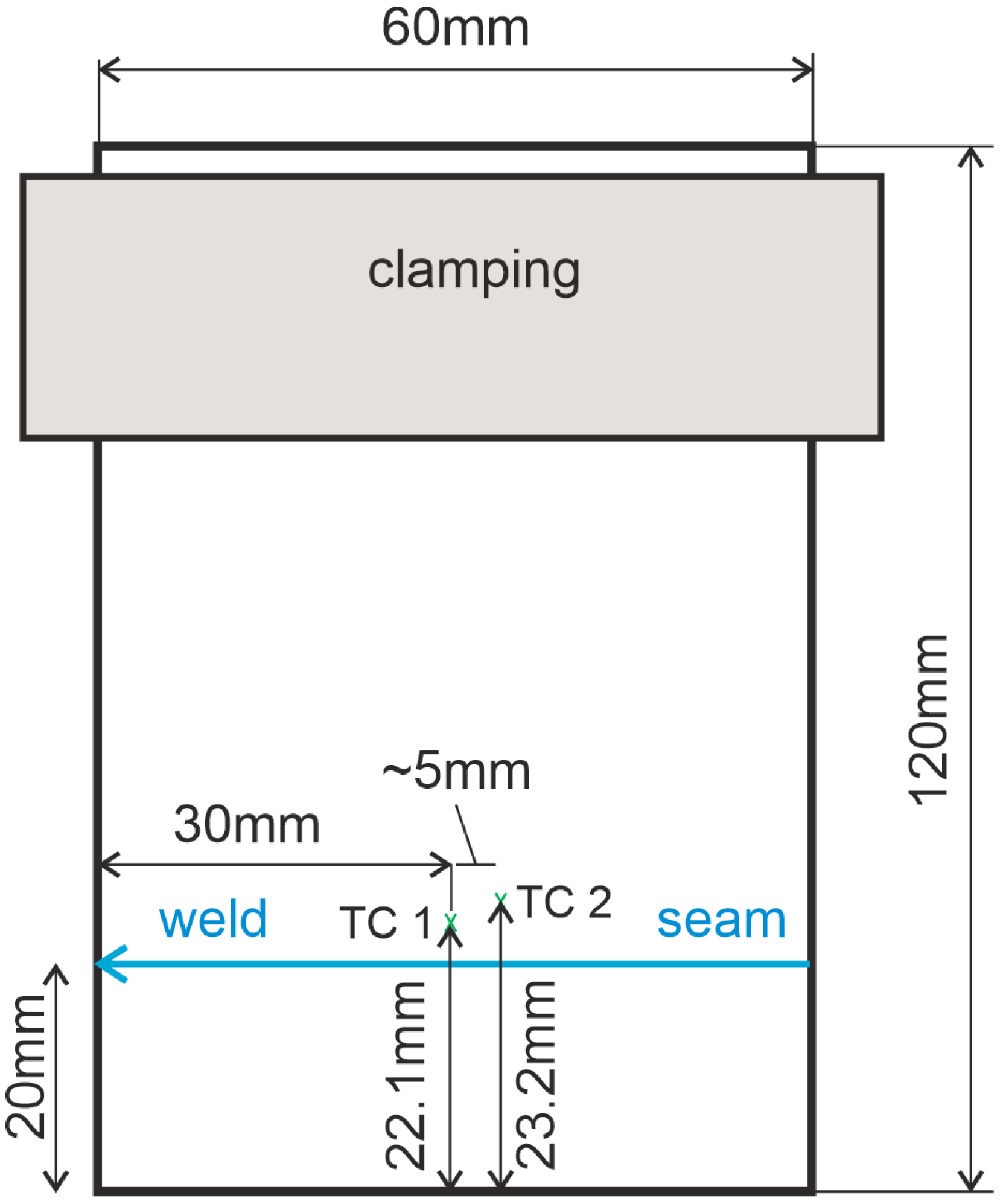
The welding sample has dimensions of $120\times 60{\mathrm{mm}}^2$, which was clamped from one side during welding. The welding was carried out at a 20 mm distance to the free edge of the sheet parallel with it. The temperature development during the welding process and the cooling was measured with two thermocouples (TC1 and TC2) located at 30 mm and 35 mm to the end position of the laser and 2.1 mm and 3.2 mm to the middle line of the weld, respectively, as shown in Figure 1.

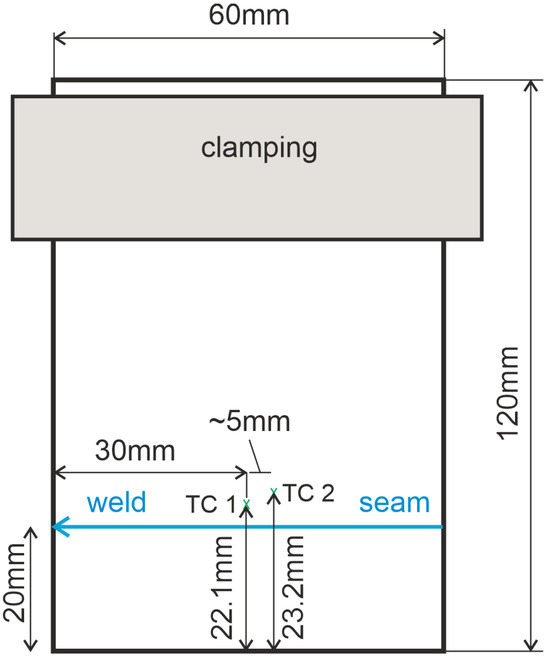
Figure 1. Schematic representation of welding setup for the temperature measurement.

3. CFD Simulation and Material Parameters

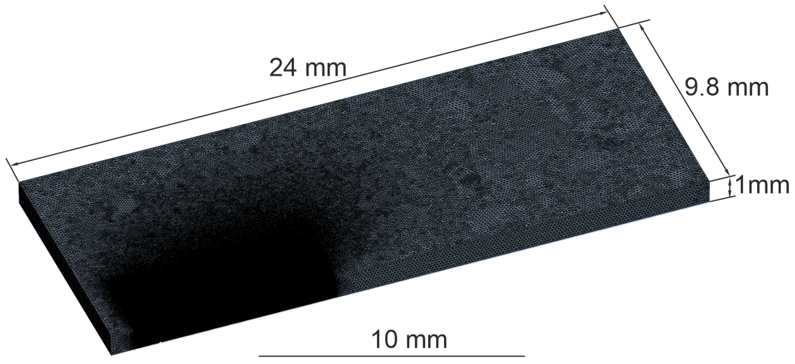
The proposed mathematical model in this paper was implemented and solved with the commercial software ANSYS Fluent (Version 2023 R1). In addition, the CFD simulation of full-penetration keyhole laser beam welding was used to obtain the weld pool geometry by considering the most relevant physical effects, such as Marangoni and natural convection, fusion heat, and temperature-dependent material properties up to the evaporation temperature. The geometrical dimensions of the computational domain were 24 mm × 9.8 mm × 1 mm (see Figure 2). A symmetry plane was applied to reduce the numerical effort and computational time, while the computational domain was discretized by a polygonal mesh of tetrahedral and triangular elements. The total number of mesh elements was about 4 × 10⁶, allowing for a minimum element size of 0.02 mm at the free surfaces and the keyhole wall to be used.

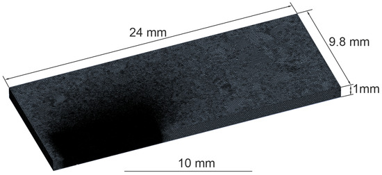
Figure 2. Mesh and dimensions of the CFD model.

Because the physical phenomena behind the laser beam welding process are strongly coupled and temperature-dependent, a highly nonlinear system of equations must be solved to obtain a solution. Here, a simplified form of the numerical model was used to guarantee numerical stability and reasonable computing time. The main assumptions in the model were similar to those used in [23] and are given as follows:

• Steady-state approach;
• Adapted size of the computational domain;
• Fixed free surface geometry;
• Approximated simplified and fixed keyhole geometry;
• Shear stress due to the interaction of metal vapor and liquid metal was not considered;
• Heat losses by radiation were neglected due to the high relation of the volume versus the surface of the plate.

Table 2 provides a summary of the material properties utilized in the model, which are temperature-dependent; see Figure 3.

Table 2. Material properties for austenitic stainless steel 1.4301 used in the CFD simulation, adapted from [24,25].

Material Property	Symbol	Value	Unit
Mass density	$\rho$	8030	kg m−3
Melting temperature	$T_{melt}$	1733	K
Evaporation temperature	$T_{evap}$	3000	K
Latent heat of fusion	$H_f$	$2.47·{10}^5$	J kg−1
Marangoni coefficient	$\partial \gamma /\partial T$	$-4.3·{10}^{-4}$	N m−1 K−1
Heat transfer coefficient (air)	h	15	W m−2 K−1
Material properties at  $T_{melt}$
Mass density	$\rho$	6900	kg m−3
Dynamic viscosity	$\eta$	$6.2·{10}^{-3}$	Pa s
Thermal conductivity	$\lambda$	150	W m−1 K−1
Specific heat capacity	$c_p$	800	J kg−1 K−1

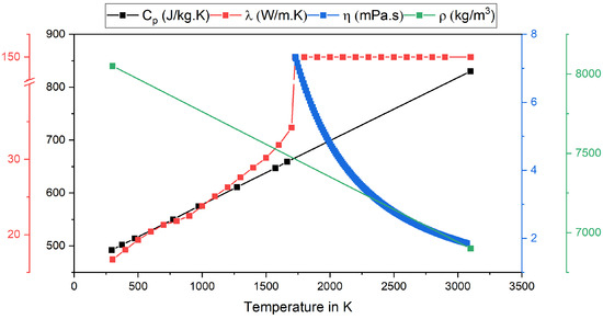
Figure 3. Temperature-dependent material properties, adapted from [24,25].

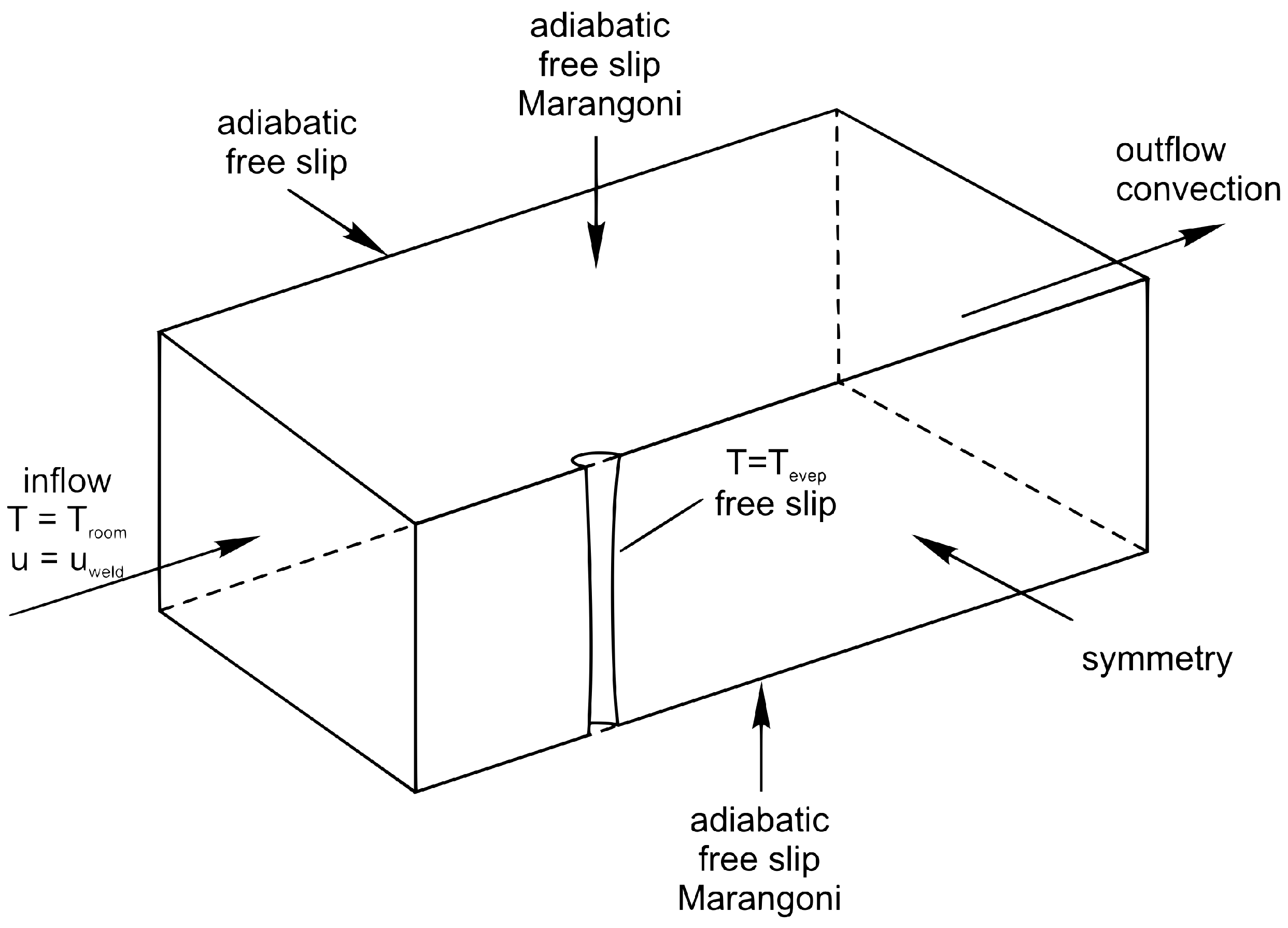
The velocity, pressure, and temperature fields of the incompressible flow were approximated by the numerical solution of the mass, the momentum, and the energy conservation equations by making use of the simulation framework of ANSYS Fluent. The numerical setup including the geometry of the workpiece and the initial state, and the boundary conditions can be seen in Figure 4. Note that the heat input was taken into account as a Dirichlet boundary condition at the keyhole surface by setting the nodal temperature equal to the evaporation temperature, instead of using a classical distributed heat source model (as will be discussed later on). A turbulent flow pattern, based on both the high velocities’ upper and lower sides—caused by the Marangoni-driven flow—and the influence of the keyhole geometry on the flow, was included by combining the Reynolds-averaged Navier–Stokes (RANS) equations with the k turbulence model. Natural convection- and buoyancy-driven flows due to gravity were considered by the Boussinesq approximation and the enthalpy–porosity technique was applied to simulate the solid–liquid phase transformation. The heat conductivity was modified by the Kays and Crawford heat transport turbulence model and accounts for the amount of produced turbulent heat conductivity. To assume the latent heat of fusion by the solid–liquid and liquid–solid phase transformation, the method of apparent heat capacity was included.

Figure 4. Boundary condition of the CFD model.

CFD Results

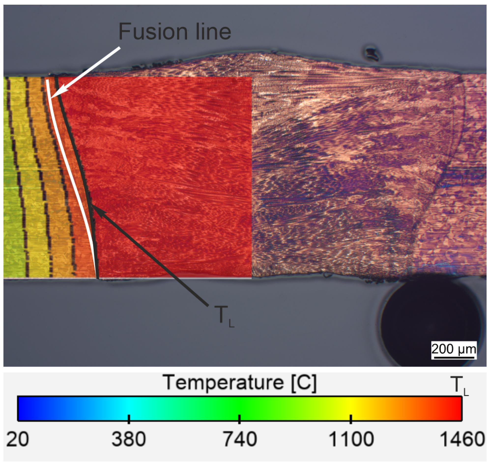
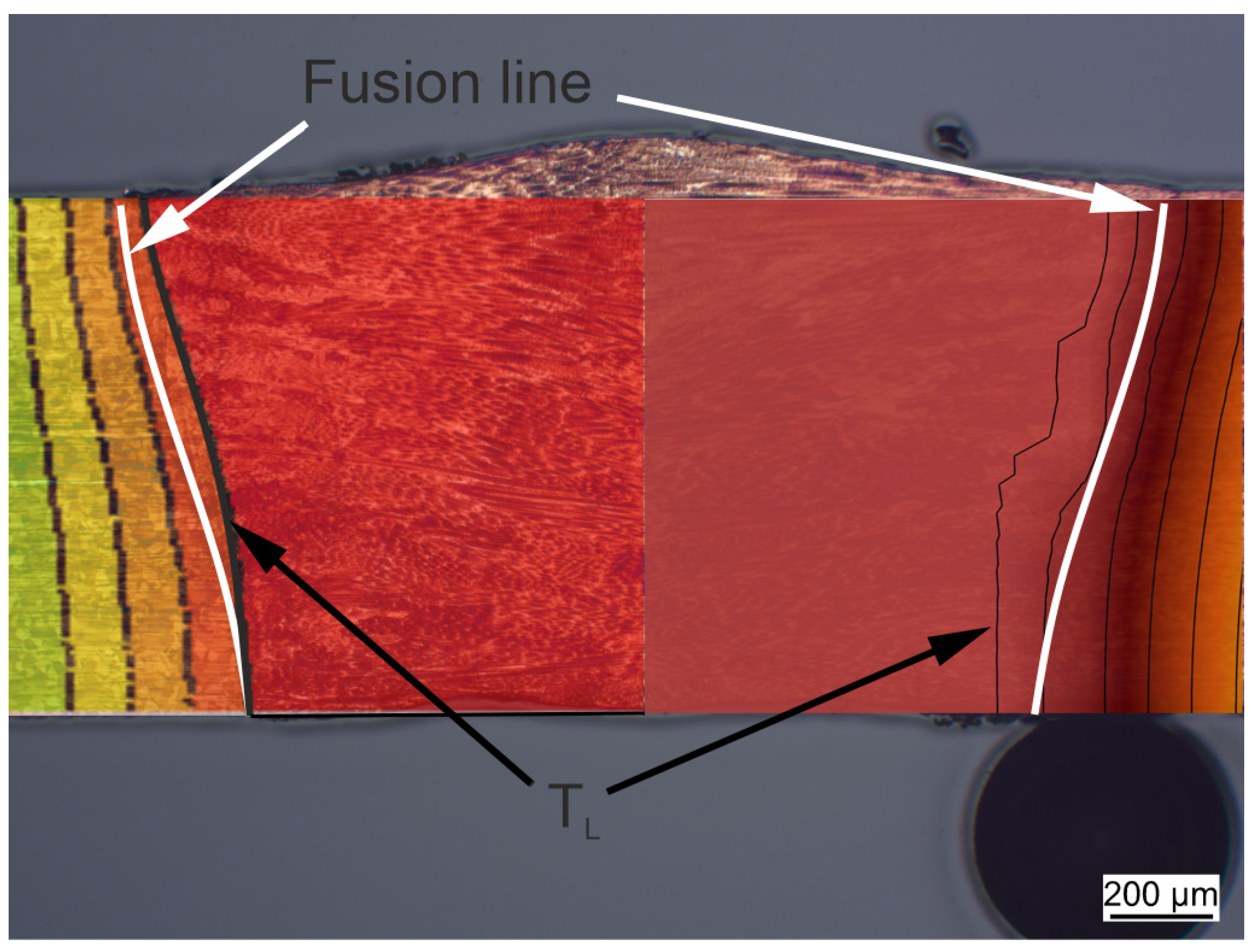
Figure 5 shows the comparison of the melt pool in cross-section between the experiment and the CFD simulation. A slight difference can be observed when comparing the melting line shown in the white line and the melting isotherm (TL) shown in the black line. However, the fused zone matches closely with the experiment, with an error of less than 5%.

Figure 5. Comparison of the fused zone between the experiment and CFD model. The white line represent the fusion line in experimental cross-section; the first black line corresponds to the liquidus temperature $T_{\mathrm{L}}=1460°\mathrm{C}$.

The experimentally observed time–temperature curves, recorded at two distances from the weld centerline (TC 1 and TC 2), are compared directly with the simulated time–temperature curves in Figure 6b. This comparison highlights the relationship between the measured maximum temperature and the thermocouples’ distance from the weld centerline. As expected, an increase in this distance leads to a corresponding decrease in the recorded maximum temperature.

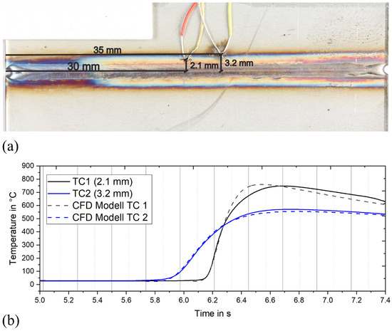
Figure 6. (a) Location of the thermocouples TC1 and TC2 for temperature measurements at the welding specimen; (b) measured and calculated temperature cycles at the corresponding points TC1 and TC2.

4. A Physically Motivated Heat Source Model

Based on the CFD simulations in Section 3, a new physically motivated heat source model is developed in this work. Alternative to the existing model described in [22], which presents a heat source model based on Dirichlet boundary conditions, we aim for the definition of a heat source term directly, which is more reasonable from the physical point of view. Similar to the mentioned model in [22], the main goal is to develop a model that describes the temperature distribution in the heat-affected zone and not the temperature states and physical effects in the melting pool. Therefore, we aim at achieving a constant temperature in the melting pool, which resembles the liquidus temperature through a suitable modification of the heat source term. Additionally, the heat source term is restricted by a physical limitation, e.g., related to the power of the laser beam.

4.1. Material Modeling for Thermal Problem

This section gives an overview of the governing balance equation, as well as the finite-element formulation used in this work. Due to the fact that this is a thermal problem, many parameters relating to temperature are used in the derivation. These are generally expressed in degrees Celsius. In places where it is absolutely necessary to use the temperature in Kelvin, this is specifically indicated. A purely thermal problem is investigated, with the energy balance given by

$$\rho r-\mathrm{div}\left(\mathit{q}\right)+\rho \theta \frac{{\partial }^2\psi }{\partial {\theta }^2}\dot{\theta }=0.$$

(1)

Here, $\rho$ denotes the density in $\frac{\mathrm{kg}}{{\mathrm{m}}^3}$, r the heat source in $\frac{\mathrm{W}}{\mathrm{kg}}$, $\mathit{q}$ the heat flux in $\frac{\mathrm{W}}{{\mathrm{m}}^2}$, $\psi$ the Helmholtz free energy in $\frac{J}{\mathrm{kg}}$, and $\dot{\theta }$ reflects the temporal derivative of the temperature. Furthermore, we assume the free energy function, adapted from [26], for a purely thermal problem as

$$\widehat{\psi }\left(\theta \right)=-c\left[\theta ln\left(\frac{\theta }{{\theta }_0}\right)-\theta +{\theta }_0\right],$$

(2)

in its volume-specific form. For this purpose, it is defined that $\rho \psi =\widehat{\psi }$. Moreover, c stands for the heat capacity in $\frac{\mathrm{J}}{{\mathrm{m}}^3\mathrm{K}}$. Utilizing the derivative of the free energy with respect to temperature, Equation (1) is reformulated to

$$\rho r-\mathrm{div}\left(\mathit{q}\right)-c\dot{\theta }=0.$$

(3)

Based thereon, a thermal FE model is constructed. Even though a standard FEM discretization is used in this paper, which can be found in text books, e.g., [27], we state the important equations, which differ from the standard form, for the realization of the presented heat source model. We used eight-noded hexahedral volume elements for the spatial discretization and, additionally, four-noded surface elements are utilized to account for heat loss across the outer surfaces. They share the same nodes as the outer volume elements in the FE discretization and are defined as linear quadrilaterals. The considered heat dissipation includes heat radiation and heat convection and is implemented as Robin boundary conditions; see [28]. It can be expressed as

$$\widehat{q}=\underset{{\widehat{q}}_{\mathrm{conv}}}{\underbrace{h_{\mathrm{conv}}\left({\theta }_{act}-{\theta }_{\infty }\right)}}+\underset{{\widehat{q}}_{\mathrm{rad}}}{\underbrace{\widehat{\sigma }\widehat{\epsilon }\left({\overline{\theta }}_{act}^4-{\overline{\theta }}_{\infty }^4\right)}};$$

(4)

see [29]. In this context, $\widehat{q}$ represents the heat flux over the surface in $\frac{\mathrm{W}}{{\mathrm{m}}^2}$, $h_{\mathrm{conv}}$ is the heat transfer coefficient for convection in $\frac{W}{{\mathrm{m}}^2\mathrm{K}}$, ${\theta }_{act}$ is the current temperature on the surface in $°\mathrm{C}$, ${\theta }_{\infty }$ is the ambient temperature in $°\mathrm{C}$, and ${\overline{\theta }}_{act}$ and ${\overline{\theta }}_{\infty }$ are the respective counterparts in $\mathrm{K}$. $\widehat{\sigma }$ is the Stefan–Boltzmann constant given by $5.67·{10}^{-8}\frac{\mathrm{W}}{{\mathrm{m}}^2{\mathrm{K}}^4}$, and $\widehat{\epsilon }$ is the dimensionless emissivity.

4.2. Finite-Element Discretization

For the FE discretization, Equation (1) is considered together with the boundary conditions

$$\theta =\widehat{\theta }\mathrm{on}\partial {\mathcal{B}}_{\theta }\mathrm{and}\mathit{q}·\mathit{n}=\widehat{q}\mathrm{on}\partial {\mathcal{B}}_{\widehat{q}},$$

(5)

where the boundary is decomposed following

$$\partial {\mathcal{B}}_{\theta }\cup \partial {\mathcal{B}}_{\widehat{q}}=\partial \mathcal{B}\mathrm{and}\partial {\mathcal{B}}_{\theta }\cap \partial {\mathcal{B}}_{\widehat{q}}=\varnothing .$$

(6)

Based on standard procedures, the weak form is obtained using the Galerkin method as

$$G=\underset{G^{int}}{\underbrace{{\int }_{\mathcal{B}}\rho r\delta \theta \mathrm{d}v+{\int }_{\mathcal{B}}\mathit{q}·grad\delta \theta \mathrm{d}v-{\int }_{\mathcal{B}}c\dot{\theta }\delta \theta \mathrm{d}v}}\underset{G^{ext}}{\underbrace{-{\int }_{\partial \mathcal{B}}\mathit{q}·\mathit{n}\delta \theta \mathrm{d}a}}=0,$$

(7)

where its linearization reads

$$\mathrm{Lin}G\left({\mathit{\theta }}_k,\delta \mathit{\theta },\Delta \mathit{\theta }\right)=G\left({\mathit{\theta }}_k,\delta \mathit{\theta }\right)+\Delta G\left({\mathit{\theta }}_k,\delta \mathit{\theta },\Delta \mathit{\theta }\right).$$

(8)

The increment reads

$$\Delta G={\int }_{\mathcal{B}}grad\delta \theta ·\left(-\lambda \right)·grad\Delta \theta \mathrm{d}v-{\int }_{\mathcal{B}}\delta \theta c\Delta \dot{\theta }\mathrm{d}v,$$

(9)

where the linearization of heat flow $\mathit{q}$ with the heat conduction matrix $\mathit{\lambda }$ as $\mathit{\lambda }=\mathrm{diag}(\lambda ,\lambda ,\lambda )$ and Fourier’s law are taken into account in the first integral term. The temperature is discretized using standard Lagrange shape functions $N^I$ for eight-noded hexahedral elements; see, e.g., [27]. The so-called B-matrix ${\mathit{B}}^I$ contains the derivatives of the shape functions, and $d^I$ contains the nodal temperature for node I.

With this discretization, the expressions in Equations (7) and (9) evaluated for one finite element e with the domain ${\mathcal{B}}^e$ leads to

$$G^{e,int}=\sum _{I=1}^{nen}\delta d^I\underset{r^{e,I}}{\underbrace{{\int }_{{\mathcal{B}}^e}\left({\mathit{B}}^{I,T}\mathit{q}+N^I\rho r-N^{I}c\dot{\theta }\right)\mathrm{d}v}},$$

(10)

$$\Delta G^{e,int}=\sum _I^{nen}\sum _J^{nen}-\delta d^I\underset{k^{e,IJ}}{\underbrace{{\int }_{{\mathcal{B}}^e}\left({\mathit{B}}^{I,T}\mathit{\lambda }{\mathit{B}}^J+N^{I}c\frac{1}{\Delta t}{N}^J\right)\mathrm{d}v}}\Delta d^J,$$

(11)

where Equation (10) contains the term related to the heat source r and Equation (11) takes the standard form. Here, $k^{e,IJ}$, $r^{e,I}$, and $\Delta d^J$ are the scalar entries of the stiffness matrix, right-hand side, and degrees of freedom associated with node I, respectively J. The assembly operation lead to the global system of equations given by

$$\mathit{K}\Delta \mathit{D}+\mathit{R}=\mathit{0},$$

(12)

which is solved using Newton’s method. Within the expression of the right-hand side, the term related to the heat source plays an important role here, and its treatment is discussed in Section 4.3.

For the consideration of heat loss across the outer surfaces, a Robin-type boundary condition is used. This is realized using two-dimensional surface elements on the outer surfaces of the considered domain $\mathcal{B}$, where heat loss shall be considered. Based on the discretization for the volume using hexahedral elements with linear shape functions, we used bilinear quadrilateral surface elements to discretize $G^{ext}$, leading to

$$G^{ext,\widehat{q}}=\sum _{I=1}^{nen}\delta d^I{\int }_{\partial {\mathcal{B}}_{\widehat{q}}}{\widehat{N}}^I\widehat{q}\mathrm{d}a,$$

(13)

where ${\widehat{N}}^I$ describes the bilinear shape functions and $\widehat{q}$ is the heat flux across the outer surface; see Equation (4) and $nen=4$.

Within the formulation of Equation (4), a dependency on the current temperature of the virtual work of external forces would occur and lead to an additional term in the linearization in Equation (11) and, thus, in the stiffness matrix. This is avoided by using ${\theta }_{act}={\theta }_n$ from the last converged time step as a reference temperature to calculate the heat flux $\widehat{q}$. Furthermore, this choice avoids possible variations of the surface heat flux during one time step resulting from a dependency on the current temperature. Thus, $\widehat{q}$ varies with respect to the surface temperature, but remains constant within one time step. Due to the small time step sizes necessary for the simulation, the difference is expected to be very small.

4.3. A Physically Motivated Heat Source Model Based on CFD Simulation

The heat source model presented in this paper differs from classical models, such as the conical model with a Gaussian distribution (see [10,30,31,32]), in the way in which the energy input is determined.

In its original form, the conical model defines a continuous energy input, causing the system to heat up without limitation. This could lead to temperatures within the heat source exceeding the liquidus temperature of the material. Such models are suitable for the modeling of the melting pool and typically need to be calibrated to experiments. In contrast to this, we are, rather, interested in the identification of the mushy zone and its temperature properties. Therefore, the newly developed heat source model uses data from prior CFD simulations, which have been calibrated to experimental data, and takes the geometry of the melting pool as an input, similar to the Lamé curve model in [22]. The model aims at achieving a constant temperature inside the entire melting pool, which shall be equal to the melting temperature. This is realized considering two aspects: (i) transferring the geometry of the weld pool geometry from the CFD simulation to identify all points in the FEM simulation where the heat source term needs to be altered and (ii) regulating the energy input based on an approximation of the temperature and redistribution of remaining energy.

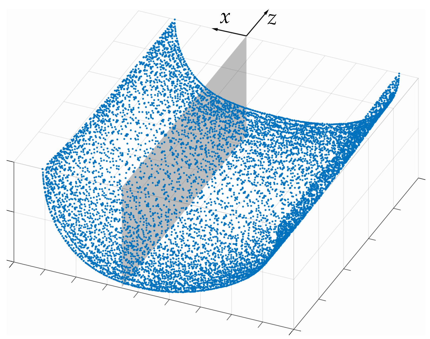
(i) The first aspect involves the geometry that corresponds to the isotherm obtained from the preceding CFD simulations; see Section 3. Thereby, an accurate representation of the molten pool bypassing a time-consuming calibration of the model parameters can be achieved. To generate this geometry, data from the CFD simulations are utilized to obtain a good fit. However, the data are available as a point cloud, as can be seen in Figure 7. In order to filter out the interior Gaussian points and, thus, associate them with the domain of the heat source, a query with the available point data is laborious. For this, it would be necessary to query for each Gaussian point whether its coordinates with respect to the local coordinate system are smaller according to the amount than the coordinates of the points of the point cloud that lie at a similar height.

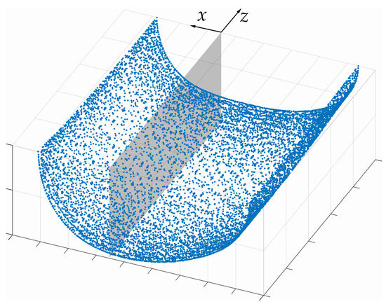
Figure 7. Extracted data from CFD simulation represented as a point cloud representing the liquidus isotherm.

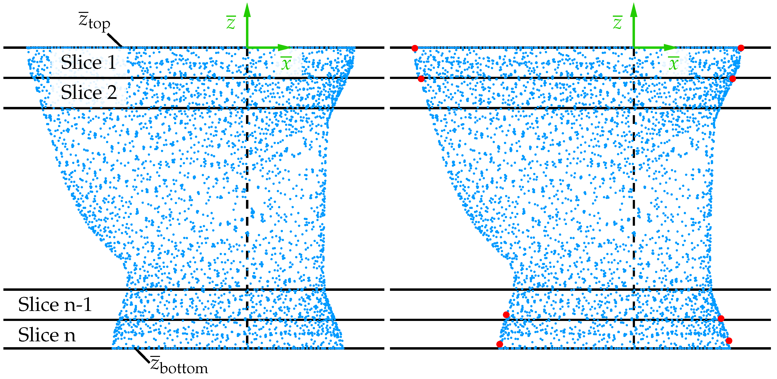
Hence, the isotherm of the liquidus temperature is approximated over the height using multiple layers based on a constant geometry over the height within one layer. The available coordinates are divided into n different layers along the thickness direction ($\overline{z}$-axis) within the range ${\overline{z}}_{\mathrm{top}}$ and ${\overline{z}}_{\mathrm{bottom}}$; see Figure 8.

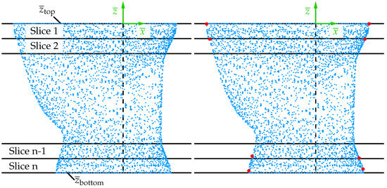
Figure 8. Exemplary representation of the division of the point cloud from the CFD simulation into different layers on the left side and schematic representation of the selection of points used to determine the double ellipse on the right side.

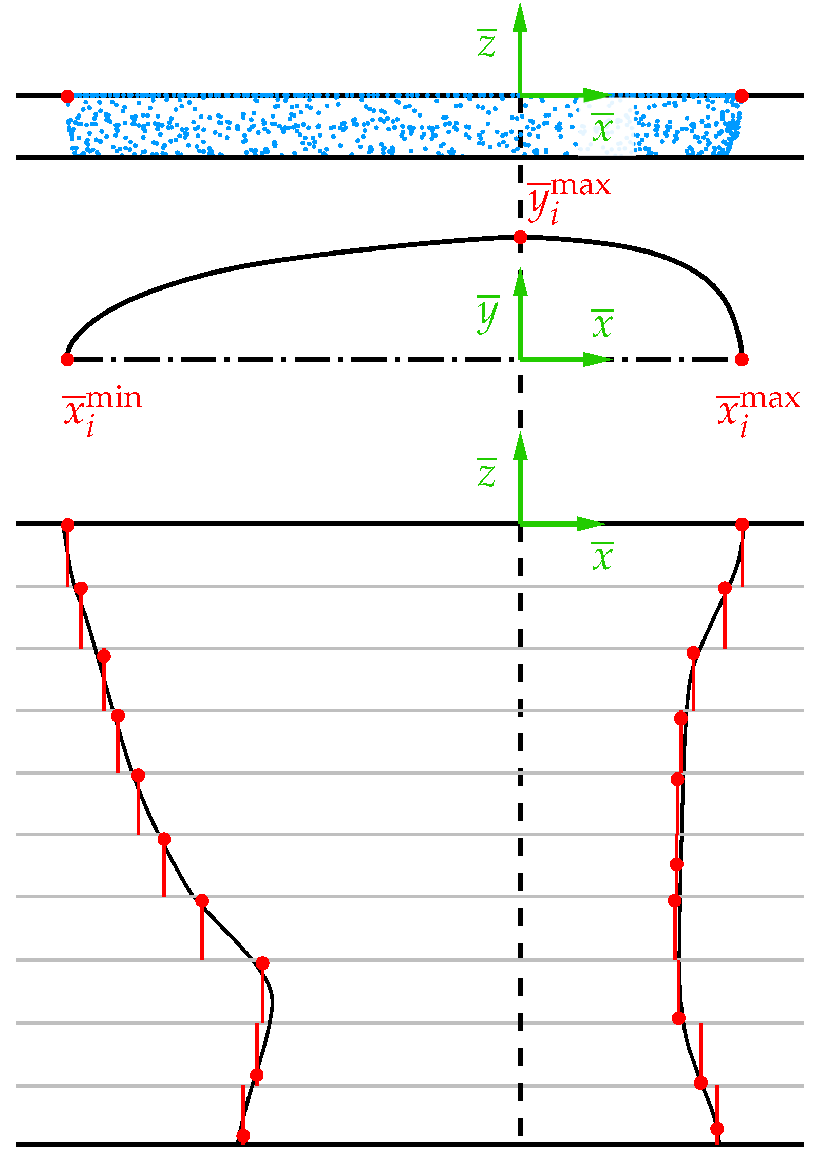
In each layer, the isotherm is approximated by two half ellipses, one in the front and one in the rear of the melting pool. The radii of these ellipses are considered constant across each layer, creating the aforementioned constant geometry. Therefore, the maximum values in the positive (${\overline{x}}_i^{\max }$), the negative (${\overline{x}}_i^{\min }$) $\overline{x}$-direction, and the $\overline{y}$-direction (${\overline{y}}_i^{\max }$) in each layer i are extracted. Due to the symmetry along the $\overline{x}$-$\overline{z}$ plane (see Section 3), only one value for the $\overline{y}$-direction is required. Additionally, multiple data points lie precisely at ${\overline{z}}_{\mathrm{top}}$ and ${\overline{z}}_{\mathrm{bottom}}$, respectively, which is why two half-ellipses are defined as layer 0 at ${\overline{z}}_{\mathrm{bottom}}$ and layer $n+1$ at ${\overline{z}}_{\mathrm{top}}$. Accordingly, at the top and bottom sides, just as for each individual layer, the maximum values ${\overline{x}}_i^{\max }$, ${\overline{x}}_i^{\min }$, and ${\overline{y}}_i^{\max }$ are extracted; see Figure 8. Thus, three radii are now available for each layer and for the upper and lower sides of the heat source. Using these values, the two half-ellipses are defined for each layer, describing the front and rear parts of the heat source separately. For the front half-ellipses, the values ${\overline{x}}_i^{\max }$ and ${\overline{y}}_i^{\max }$ are employed, while for the rear half-ellipses, ${\overline{x}}_i^{\min }$ and ${\overline{y}}_i^{\max }$ are used. Because both the front and rear parts share the same width (${\overline{y}}_i^{\max }$), a smooth transition between the parts is achieved when they are combined, as shown in Figure 9. The collected data of the radii for each layer are stored and used within the FE simulation to determine the domain of the melting pool.

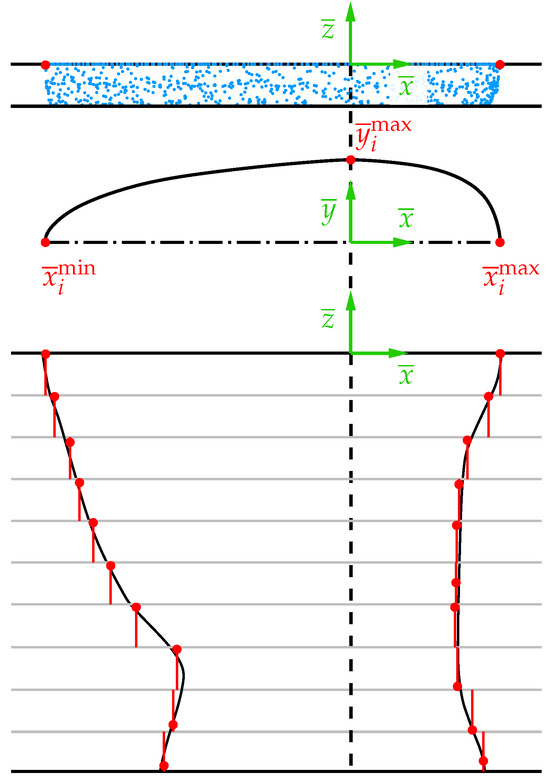
Figure 9. Illustration of the creation of a double ellipse for one layer as an example and the corresponding approximated geometry for the FE simulation.

Based on the collected data, the approximated geometry of the isotherm is used to check which Gaussian points are located inside or outside the melting pool. As mentioned before, the heat source can be divided into two parts, the front and the rear part. That is, if $\overline{x}>0$, the condition for the front part:

$${\displaystyle \frac{{\overline{x}}^2}{{\overline{x}}_i^{\max }{\left(\overline{z}\right)}^2}}+{\displaystyle \frac{{\overline{y}}^2}{{\overline{y}}_i^{\max }{\left(\overline{z}\right)}^2}}\le 1,$$

(14)

is checked, and if $\overline{x}\le 0$, the condition for the rear part:

$${\displaystyle \frac{{\overline{x}}^2}{{\overline{x}}_i^{\min }{\left(\overline{z}\right)}^2}}+{\displaystyle \frac{{\overline{y}}^2}{{\overline{y}}_i^{\max }{\left(\overline{z}\right)}^2}}\le 1,$$

(15)

is checked, because the lengths of the half ellipse for the front and rear parts are different. If the coordinates of a node satisfy one of these conditions, the node lies within the molten pool, and the corresponding energy input is determined according to Equation (26). In case the condition is not met, signifying that the node is outside the pool, no energy input is determined. The determined value of energy input is used to alter the right-hand side of the FE problem. The number of layers to approximate the geometry from the CFD simulation can be chosen arbitrarily. However, care should be taken to ensure that sufficient resolution of the geometry is achieved. The number and size of the elements in the FE simulation also play a role. For example, too coarse of a meshing can cause layers to be left out, since the height of an element is greater than the layer thickness and, thus, includes more than two layers. Accordingly, the number of elements in the height should at least correspond to the number of layers. For the applied linear hexahedral elements (see Section 4.1), there are at least two Gaussian points in one layer.

(ii) The second objective is to bound the temperature by the liquidus temperature in the region where the heat source is active, as identified based on Gaussian point data from objective (i). To achieve this, the energy input is computed based on the current temperature. Additionally, a redistribution of the energy input is used. The aim of this redistribution is to ensure that the areas that heat up more slowly are supplied with more energy during the heating process so that a constant temperature distribution in the melt pool is achieved. At first, the temperature for the current time step $t_{n+1}$ is estimated. The temperature increase from the last time step $\Delta {\theta }_n={\theta }_n-{\theta }_{n-1}$, calculated from the temperature of the last time step ${\theta }_n$ and the temperature from the penultimate time step ${\theta }_{n-1}$, is used as an approximation. Thus,

$${\theta }_{\mathrm{approx}}={\theta }_n+\Delta {\theta }_n.$$

(16)

The approximated temperature ${\theta }_{\mathrm{approx}}$ is now used in the following steps to determine the energy input for each Gaussian point. As mentioned above, energy input is regulated related to the temperature, based on the approximated temperature; see Equation (16). In order to achieve a constant temperature around the liquidus temperature, a heating phase and a holding phase are realized. The overall energy input is limited by the total amount of power provided through the laser. The total power is given by

$$Q={\int }_{v^{\mathrm{analy}}{.}_{\mathrm{HS}}}\rho r_0\mathrm{d}v.$$

(17)

Here, Q denotes the given laser power, which defines the value of $r_0$ as the maximum power density, and $v^{\mathrm{analy}}{.}_{\mathrm{HS}}$ is the volume in which the heat source is active. For the heating phase, where ${\theta }_{\mathrm{approx}}$ is below the liquidus temperature ${\theta }_{\mathrm{liq}}$, this results in an energy density of

$$\overline{R}={\overline{R}}_0=\rho r_0=\frac{Q}{v_{\mathrm{HS}}^{\mathrm{analy}.}}.$$

(18)

$\overline{R}$ describes the calculated value of the energy density used in the simulation. If the temperature rises above the liquidus temperature, the holding phase begins. During the holding phase, the temperature of the molten pool is kept constant around the liquidus temperature ${\theta }_{\mathrm{liq}}$. A distinction is made between two cases during this phase. In the first case, the temperature has only risen above the liquidus temperature in the current time step; thus, ${\theta }_n<{\theta }_{liq}$. In this case, the energy input is scaled by a factor smaller than one. The scaling is carried out by means of a linear interpolation related to the temperature. This means that the energy density is defined as

$$\overline{R}=\rho r_0\frac{{\theta }_{\mathrm{liq}}-{\theta }_n}{\Delta {\theta }_n}.$$

(19)

If the approximated temperature is equal to ${\theta }_{\mathrm{liq}}$, this value equals ${\overline{R}}_0$. Using the approximation in Equation (16), one can show that this factor must be smaller than one since it holds that

$$\begin{array}{rrrrr}& & {\theta }_{\mathrm{approx}}& >& {\theta }_{\mathrm{liq}}\\ \iff & & {\theta }_n+\Delta {\theta }_n& >& {\theta }_{\mathrm{liq}}\\ \iff & & {\theta }_n+{\theta }_n-{\theta }_{n-1}& >& {\theta }_{\mathrm{liq}}\\ \iff & & {\theta }_n-{\theta }_{n-1}& >& {\theta }_{\mathrm{liq}}-{\theta }_n\\ \iff & & 1& >& \frac{{\theta }_{\mathrm{liq}}-{\theta }_n}{{\theta }_n-{\theta }_{n-1}}.\end{array}$$

(20)

In the second case, both the approximated temperature and the temperature from the last time step are above the liquidus temperature. In order to achieve a constant temperature around ${\theta }_{\mathrm{liq}}$, the energy input must be switched off, which means that

$$\overline{R}=0$$

(21)

applies. As a result, no further energy is added to the system at the Gaussian point, and the point cannot heat up any further. Within the described scheme, the total energy input Q is not achieved when any point in the system receives a modified energy input $\overline{R}<{\overline{R}}_0$. Due to heat conduction within the domain of the melt pool, these points will be located rather in the center of the melt pool, whereas points closer to the boundary may still have a lower temperature. For these points with a lower temperature, the energy left free from $\overline{R}<{\overline{R}}_0$ is redistributed in order to achieve a constant temperature within the melt pool faster according to the following scheme. The total energy entering the system based on the FEM simulation is computed at the end of each time step based on

$$Q^{\mathrm{FEM}}={\int }_{v_{\mathrm{HS}}^{\mathrm{FEM}}}\overline{R}\mathrm{d}v=\sum _{GP}\overline{R}\mathrm{dvol},$$

(22)

where the analytical integral is reformulated based on a typical Gaussian integration used in the FEM. Here, the total volume in which the heat source is applied is computed as

$$v_{\mathrm{HS}}^{\mathrm{FEM}}=\sum _{GP}\mathrm{dvol},$$

(23)

where dvol represents the contribution from each Gaussian point within the heat source volume. It should be noted that $v_{\mathrm{HS}}^{\mathrm{FEM}}$ may differ from $v_{\mathrm{HS}}^{\mathrm{analy}}.$. This is because $v_{\mathrm{HS}}^{\mathrm{FEM}}$ depends on the Gaussian points and, therefore, on the location and discretization. This means that $v_{\mathrm{HS}}^{\mathrm{FEM}}=v_{\mathrm{HS}}^{\mathrm{analy}}.$ only applies to an infinitely fine mesh. It holds that $Q\ge Q_{\mathrm{FEM}}$. Thus, the average energy density is computed as

$${\overline{R}}_{\mathrm{used}}=\frac{Q^{\mathrm{FEM}}}{v_{\mathrm{HS}}^{\mathrm{FEM}}}.$$

(24)

Using this value, a factor $fac{t}_Q$ for the modification is computed as

$$fac{t}_Q=\frac{{\overline{R}}_0}{{\overline{R}}_{\mathrm{used}}}=\frac{Q·v_{\mathrm{HS}}^{\mathrm{FEM}}}{Q^{\mathrm{FEM}}·v_{\mathrm{HS}}^{\mathrm{analy}.}},$$

(25)

which is used in the next time step to redistribute the difference in power between Q and $Q_{\mathrm{FEM}}$ to all Gaussian points. Then, we modify the energy density at the Gaussian points as

$${\overline{R}}_{\mathrm{mod}}=fac{t}_Q·\overline{R}.$$

(26)

This modification only applies if ${\theta }_{\mathrm{approx}}\le {\theta }_{\mathrm{liq}}-\mathrm{tol}$, where $\mathrm{tol}$ is chosen as $2\mathrm{K}$, and it is limited to a factor of $\max \left(fac{t}_Q\right)=5$. Therefore, only areas that have not yet reached ${\theta }_{\mathrm{liq}}$ are influenced and receive a higher energy density, leading to a faster heating.

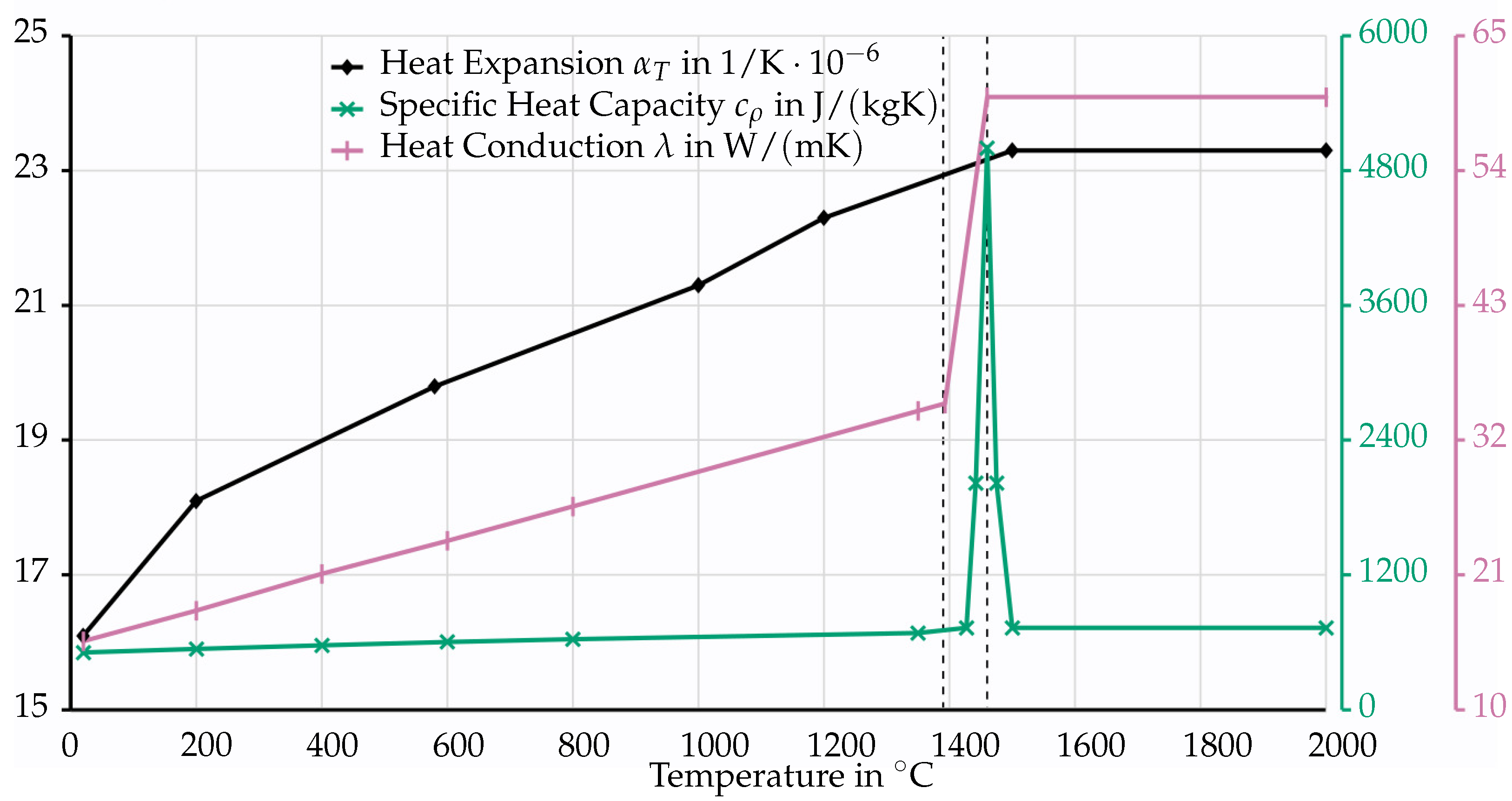
In addition to the two main aspects, the material behavior of the liquid phase is approximated based on temperature-dependent material parameters, as shown in Figure 10.

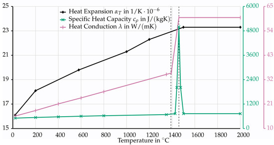
Figure 10. Material parameters for the used austenitic chrome-nickel steel 1.4301. The data originate from the software Sysweld. The first dashed line visualizes the solidus temperature ${\theta }_{\mathrm{sol}}$, and the second dashed line visualizes the liquidus temperature ${\theta }_{\mathrm{liq}}$.

5. Numerical Examples

To validate the proposed physically based heat source model, it will be analyzed and compared to experimental data, the CFD simulation, and an FE simulation using the Lamé model in the following section. Therefore, the boundary-value problem (BVP) and the material and process parameters are introduced and discussed. The described FE formulation and heat source model have been implemented in an in-house FE code based on the software FEAP (Version 8.2); see [33].

5.1. Material and Process Parameters

The numerical examples given later in this paper (see Section 5.2 and Section 5.3) reflect a thin metal plate of austenitic chrome-nickel steel (1.4301). The chemical composition of the used material is depicted in Table 1. For this composition, the solidus temperature ${\theta }_{\mathrm{sol}}$ is $1390°\mathrm{C}$ and the liquidus temperature ${\theta }_{\mathrm{liq}}$ is $1460°\mathrm{C}$, which were determined using JMatPro (Version 13.2); see [34].

The material parameters utilized in this study were obtained from the software Sysweld (https://www.esi-group.com/products/sysweld, accessed on 18 March 2024) and are presented graphically in Figure 10. They apply to a temperature range between $0°\mathrm{C}$ and $2000°\mathrm{C}$. For the material density, no direct data are available. Thus, it was assumed to remain constant with temperature and set at a value of $7919\frac{\mathrm{kg}}{{\mathrm{m}}^3}$. This specific density value, corresponding to $20°\mathrm{C}$, was extracted from [35]. While the material parameters are provided only for certain temperatures, it is necessary to consider the intermediate temperature ranges during the simulation. To account for this, a linear interpolation of the values was conducted using

$${\theta }_k<\theta \le {\theta }_{k+1}\Rightarrow p=p_k+{\displaystyle \frac{p_{k+1}-p_k}{{\theta }_{k+1}-{\theta }_k}}·\left(\theta -{\theta }_k\right)\mathrm{with}p={\alpha }_{\mathrm{T}},c_{\rho },\lambda .$$

(27)

The equation utilizes ${\theta }_k$ and ${\theta }_{k+1}$ to represent temperatures with known parameters $p_k$ and $p_{k+1}$, respectively, whereas p is the sought parameter at a given temperature $\theta$. Employing Equation (27), we can determine the parameter p for an intermediate temperature. The energy rate (power) Q for the modified volumetric heat source model was set at $1\mathrm{kW}$.

A comparison of the material parameters from Figure 3 and Figure 10 shows that the values for the CFD and FEM simulation differ. However, this can be explained as follows. The specific heat capacity $c_{\rho }$ forms a singularity at the melting temperature. To map this, the integral is formed over a certain temperature range. This temperature range differs in the models in order to achieve numerical stability in both cases. For thermal conductivity $\lambda$, there is a relatively large jump in the range of the melting temperature. While the CFD model also requires material parameters above the melting temperature, the temperature range up to the melting temperature is of interest in the FE model. If the values up to this temperature are compared, no major differences are recognizable. Finally, a constant density $\rho$ is assumed in the FE simulation and a temperature-dependent density in the CFD simulation. Since the determination of the heat source is based on a volume-specific formulation, the density only has an influence on the determination of the heat capacity via $c=\rho c_{\rho }$. However, this has no influence on the final temperature distribution.

5.2. Analysis of Steady Conical Heat Source

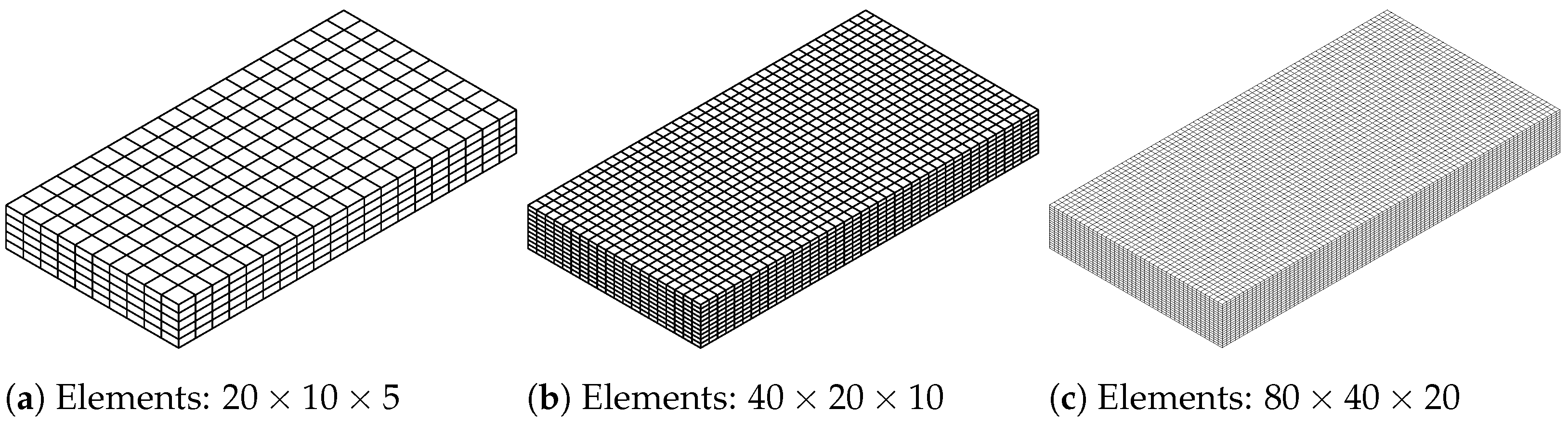
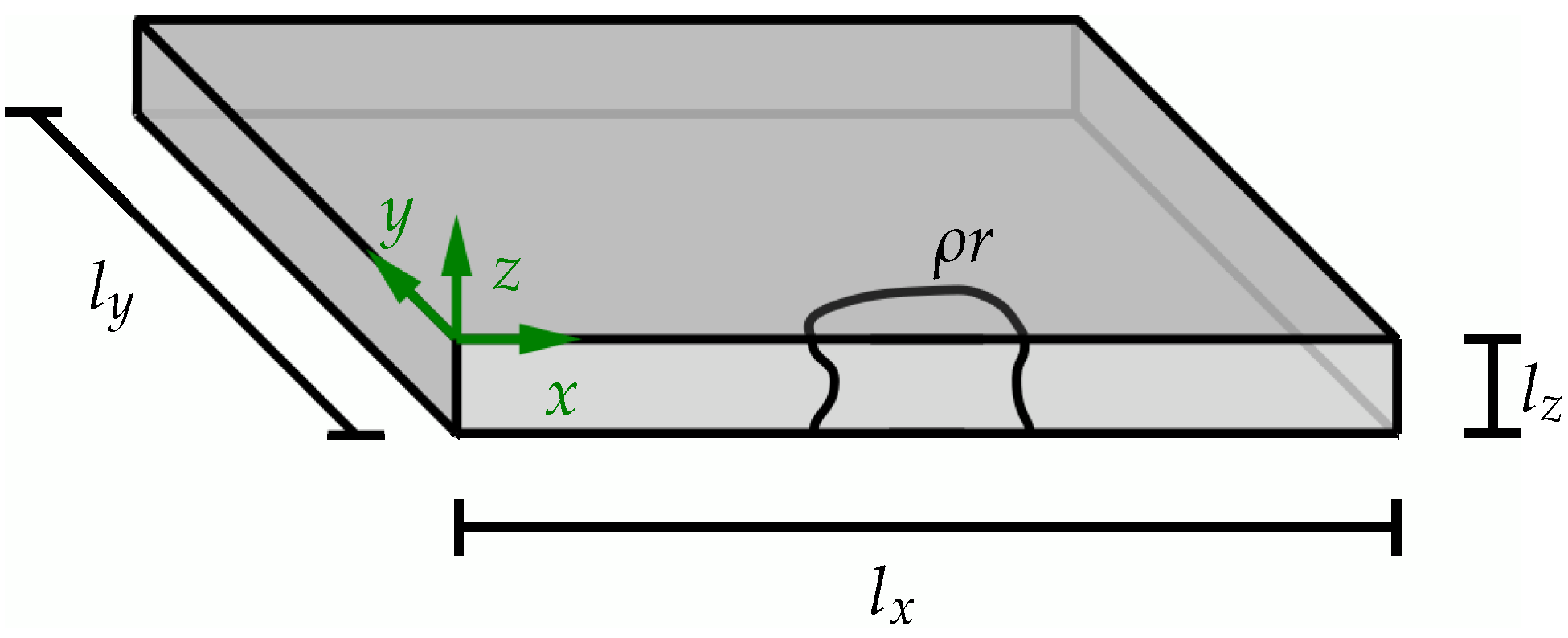
The presented heat source model was investigated with regard to the sensitivity with respect to the time step size. In addition, the spatial discretization was analyzed in terms of its influence on the temperature distribution and the ability to approximate the prescribed isotherm of ${\theta }_{\mathrm{liq}}$. Therefore, the temperature distribution coming from a steady heat source was determined for three different discretizations and three different time step sizes ($\Delta t\in \left\{0.01\mathrm{s};0.001\mathrm{s};0.0001\mathrm{s}\right\}$). A simplified boundary-value problem with spatial dimensions of $l_x=10\mathrm{mm}$, $l_y=5\mathrm{mm}$, and $l_z=1\mathrm{mm}$ was assumed. It was discretized with 20 elements × 10 elements × 5 elements, 40 elements × 20 elements × 10 elements and with 80 elements × 40 elements × 20 elements; see Figure 11.

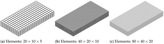
Figure 11. Discretizations of the analysis of the steady conical heat source model.

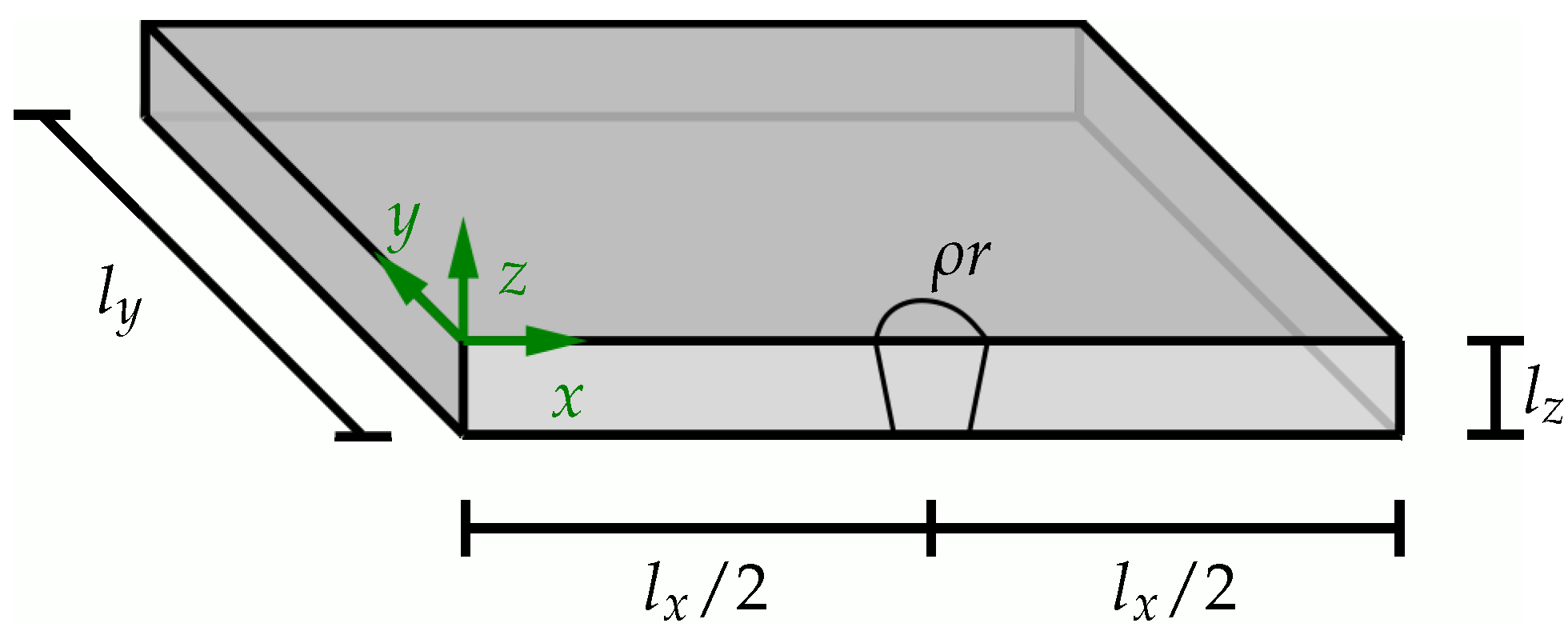
In this simplified example, the geometry of the molten pool is represented by a cone with an upper radius of $1.2\mathrm{mm}$ and a lower radius of $0.8\mathrm{mm}$. To evaluate the temperature distribution without the influences of the boundaries, the heat source is located at the center of the examined workpiece at $x=5\mathrm{mm}$. This is illustrated graphically in Figure 12. All surfaces, except the assumed symmetry plane along the weld seam at $y=0$, were considered for the Robin boundary conditions (see [28]) to mimic heat transition. The symmetry plane was used to utilize the fact that no heat exchange takes place at this plane. Therefore, the symmetry condition was applied in order to only have to simulate half of the system and, thus, save computing time. The heat transfer coefficient h was set to $15\frac{\mathrm{W}}{{\mathrm{m}}^2\mathrm{K}}$ and the emissivity $\widehat{\epsilon }$ to $0.85$.

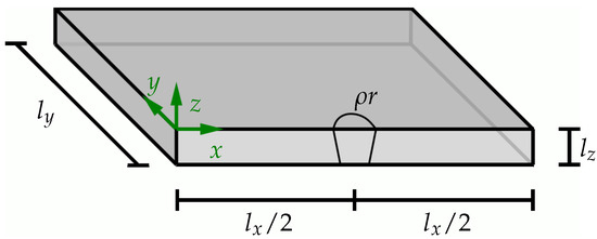
Figure 12. BVP for the analysis of temperature distribution for steady conical heat source.

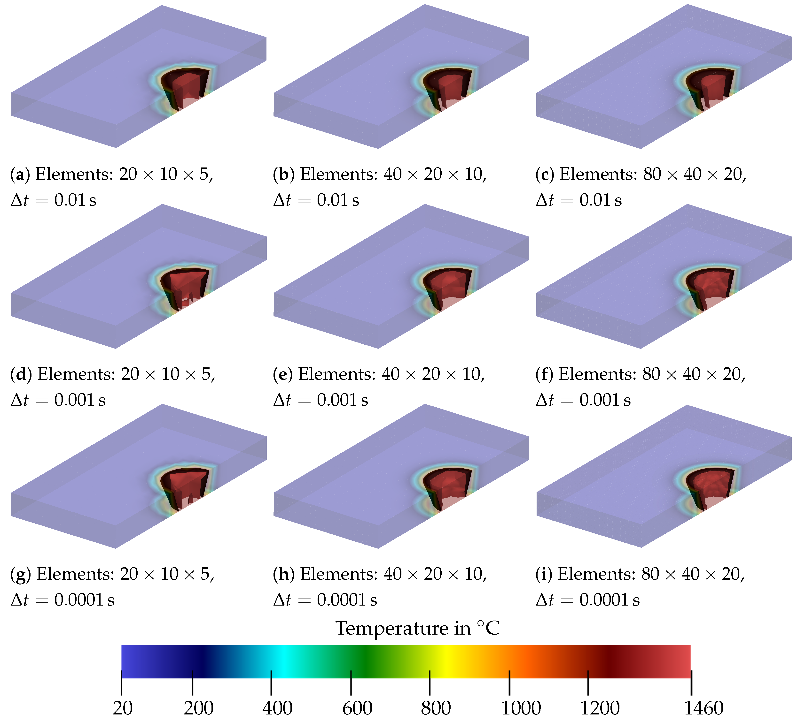
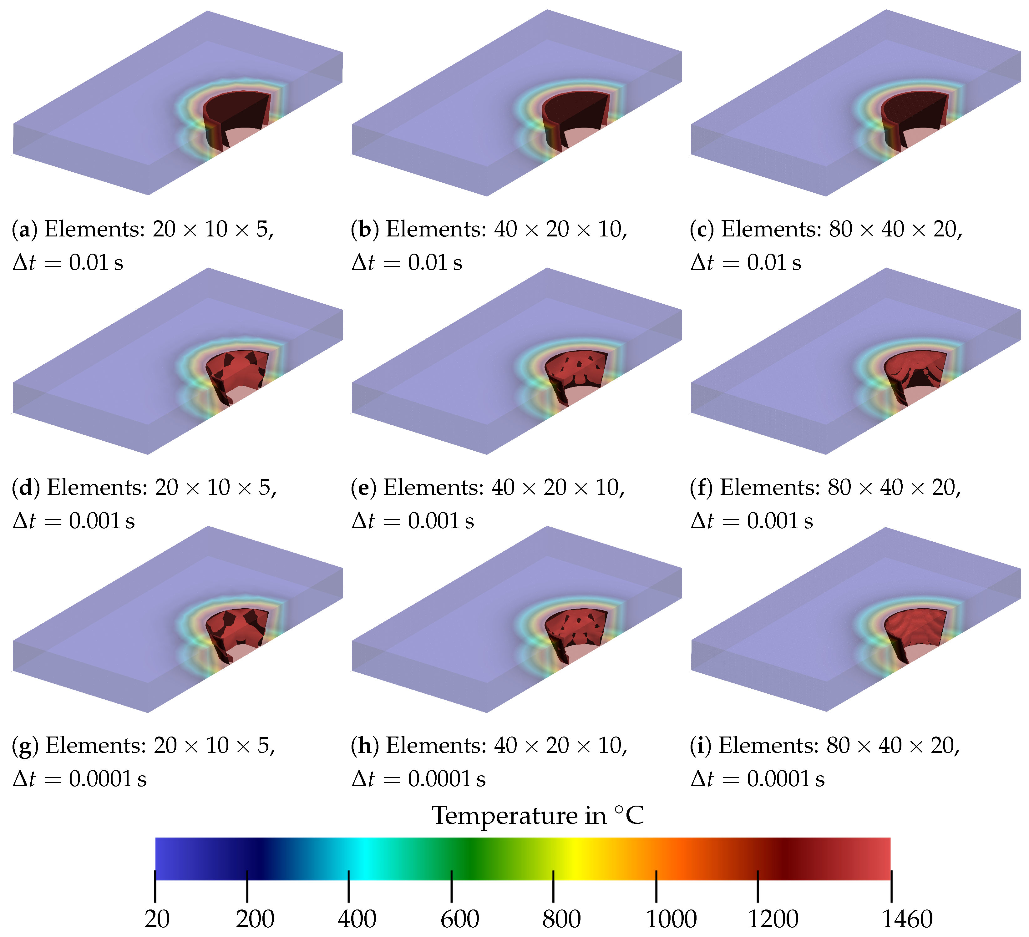
The results of the analysis are shown in Figure 13, Figure 14 and Figure 15 at different points in time. The isotherm is shown as the red surface, and the black cone serves as a comparison and represents the boundary of the melt pool. It is shown that, for any combination of time step size and discretization, the heat source does not achieve a fully heated melt pool at $t=0.05$ s up to ${\theta }_{\mathrm{liq}}$. This can be recognized by the fact that, in Figure 13, the isotherm is still within the black cone for all cases. It can be seen that, for a time increment of 0.01 s, the temperature distribution progresses more slowly than for smaller time increments. Furthermore, two isotherms for ${\theta }_{\mathrm{liq}}$ occur for a rough meshing with a smaller time step; see Figure 13d,g. This is assumed to arise due to coarse meshing. In addition to that, it can be seen that, with finer meshing (see Figure 13b,c), the shape of the isotherm becomes smoother.

Figure 13. Comparison of the temperature distribution for a steady heat source for different time step sizes and discretizations at $t=0.05\mathrm{s}$.

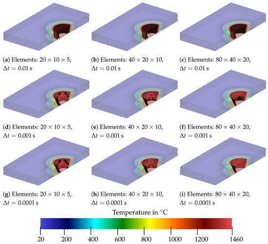
Figure 14. Comparison of the temperature distribution for a steady heat source for different time step sizes and discretizations at $t=0.1\mathrm{s}$.

Figure 15. Comparison of the temperature distribution for a steady heat source for different time step sizes and discretizations at $t=1.5\mathrm{s}$.

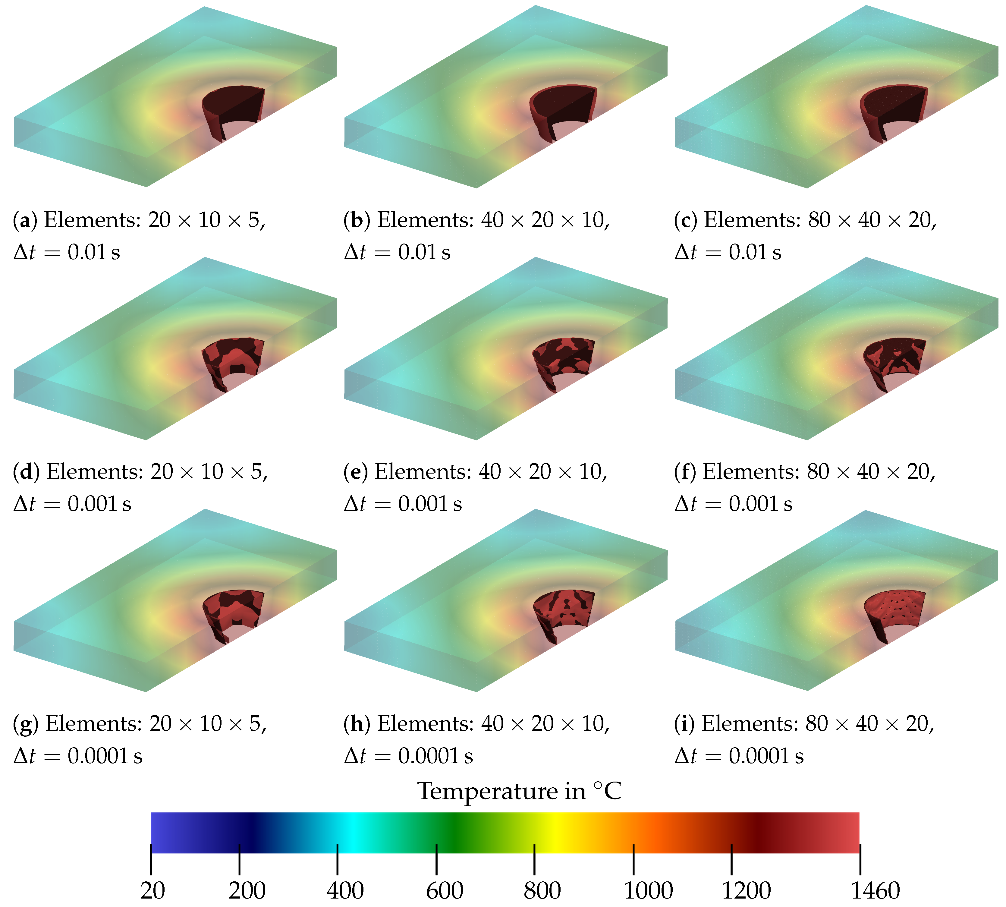
At $t=0.1$ s, even the coarsest mesh approaches a rounder shape, as can be seen in Figure 14a,d,g. However, it can also be observed in Figure 14a–c that, for a time step of $0.01$ s, the range of the isotherm is already larger than the specified geometry of the melt pool. This does not occur for $\Delta t=0.001\mathrm{s}$ and $\Delta t=0.0001\mathrm{s}$, where the isotherm already matches the cone quite well. In Figure 15a–c, all time step sizes lead to a somewhat feasible approximation of the cone, with $\Delta t=0.01\mathrm{s}$ showing the largest deviation. From this analysis, it was concluded that a time step size of at least $\Delta t=0.001\mathrm{s}$ should be used. No major differences can be seen between the two smaller time step sizes. Although the approximation to the cone appears to be somewhat more accurate with a smaller time step size, the results with a time step size of $0.001$ s also look promising.

For the different discretizations, it follows that the coarsest mesh gives an angular shape of the isotherm, and therefore, the results are too imprecise for our purposes. Although the finest mesh naturally provides the best representation of the isotherm as a cone, the fineness of the mesh is also associated with high computing times. If one compares the medium mesh with the finest mesh, differences are recognizable. It can be summarized that a sufficiently fine mesh must be used so that the specified geometry can be mapped appropriately. This is especially of importance when more complex geometries are used compared to the cone. Thus, it can be concluded that the medium meshing with a time step of $0.001$ s can provide sufficiently accurate results for the steady heat source. In view of a moving heat source, a smaller time step size is considered in the following to describe the temperature evolution accurately. Furthermore, due to the more complex isotherm geometry we will consider, an intermediate mesh size between medium and fine is used for the spatial discretization.

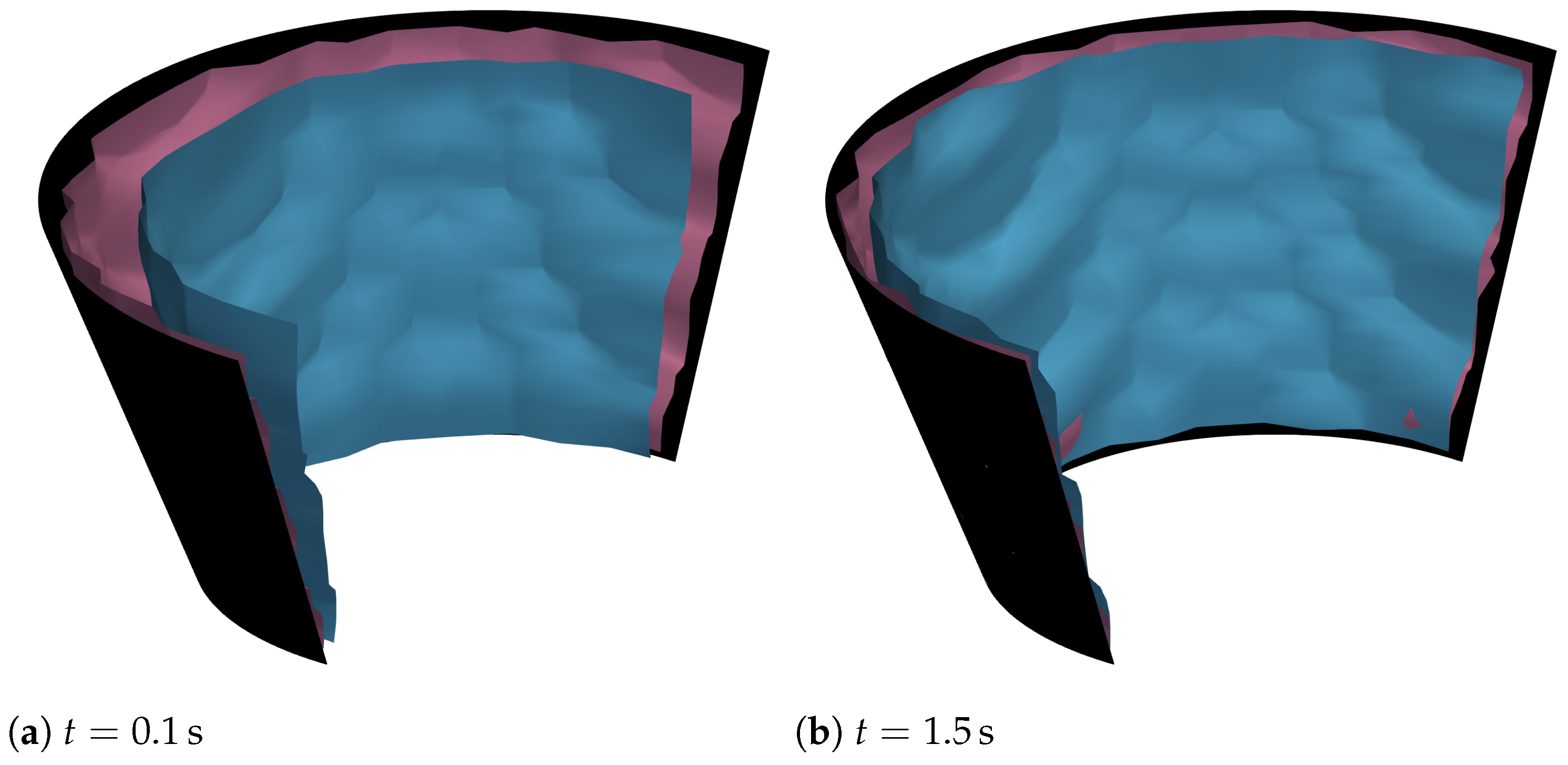
The significance of the redistribution of energy by means of the factor $fac{t}_Q$ is discussed in the following. Therefore, the results obtained above are compared with a heat source model that does not use a redistribution of energy. In this case, $fac{t}_Q$ is always 1 and cannot be changed. This means that the redistribution of energy does not take place and the energy input is only determined using Equation (19). Figure 16 shows the isotherms of the liquidus temperature of both cases for two points in time. We compare here a discretization of $80\times 40\times 20$ elements and a time step width of $\Delta t=0.0001\mathrm{s}$. The purple surface corresponds to the case in which $fac{t}_Q$ is variable, and the light blue surface corresponds to the case in which $fac{t}_Q$ is always equal to 1. At both points in time, it can be seen that the blue surface has a smaller size than the purple surface.

Figure 16. Comparison of the isotherm of the liquidus temperature with the redistribution of energy (purple surface) and without the redistribution of energy (blue surface) in relation to the given heat source geometry (black cone) for different points in time.

It can also be seen that, for the purple surface, a good result for approximating the specified geometry of the heat source is already available after $0.1$ s, whereas in the second case, the blue surface still expands over time and only approaches the cone after $1.5$ s. This allows the conclusion that $fac{t}_Q$ has a significant influence on the temperature distribution. The distribution of the energy ensures that the areas with a lower temperature heat up much faster, resulting in a shorter heating phase. In addition, the energy input $\overline{R}$ is shown in Figure 17. The results from the calculation were used, which used a spatial discretization of 80 elements × 40 elements × 20 elements and a time step size of $\Delta t=0.0001\mathrm{s}$. The results are shown for two different points in time and for the case that the energy redistribution takes place via $fac{t}_Q$ and for the case that the energy redistribution does not take place.

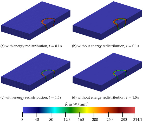
Figure 17. Representation of the energy input $\overline{R}$ for cases with and without energy redistribution at various time points.

The figure clearly shows that the energy input decreases over time. For both cases of energy input, it is, therefore, evident that the red areas, which means an energy input of $314\frac{\mathrm{W}}{{\mathrm{mm}}^3}$ and more, become smaller. The reason why the red areas are more pronounced for the first case is that the factor $fac{t}_Q$ can increase up to 5; see Section 4.3. Accordingly, maximum values of approximately $1500\frac{\mathrm{W}}{{\mathrm{mm}}^3}$ are possible. It can also be seen that, if there is no redistribution of energy, the area of maximum energy input lies further inside the cone. This is consistent with the results that can be inferred from Figure 16. The redistribution of energy ensures that the areas of lower temperature heat up more quickly.

5.3. Moving Heat Source

The numerical realization of the laser beam welding process involves defining an appropriate boundary-value problem. In this regard, the boundary-value problem was set up in relation to the experiments conducted in Section 2. This is shown in Figure 18. We selected a subsection of the real boundary-value problem given in the experiment, which ensures that all regions of relevant temperatures are included.

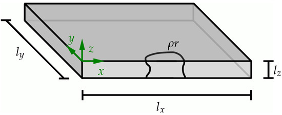
Figure 18. BVP for moving physically based heat source.

The boundary-value problem has a height $l_z$ of $1\mathrm{mm}$, a length $l_x$ of $60\mathrm{mm}$, and a width $l_y$ of $31.444\mathrm{mm}$. At $y=0$, a plane of symmetry is assumed (compare Section 2), which is where the center line of the weld seam is located. This is in line with the CFD simulation in Section 2. On the outer surface, the heat flux must be considered, which represents convection and radiation. For these thermal constraints, Robin boundary conditions were used (see [28]), which were adapted from [29]; see also Section 4.1. In the numerical example, surface elements were applied to every side of the system except for the symmetry plane at $y=0$. A heat transfer coefficient value of $h_{\mathrm{air}}=15\frac{\mathrm{W}}{{\mathrm{m}}^2\mathrm{K}}$ and an emissivity of $0.85$ were chosen equally on all outer surfaces.

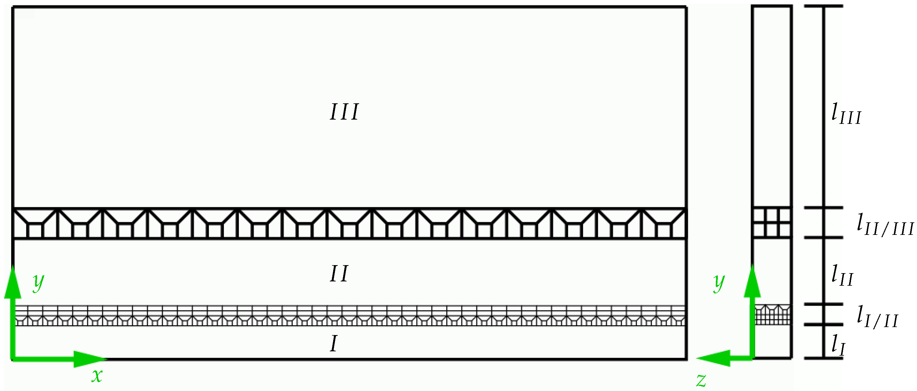
For the discretization, the software GMSH (Version 4.11.1) was used; see [36]. A structured mesh was constructed for the problem, which accounts for different mesh densities in different domains, as shown in Figure 19.

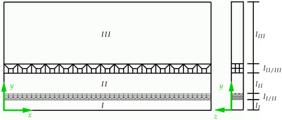
Figure 19. Overview of the differently meshed areas of the BVP including transition zones.

A total of three regions were constructed, which are connected by two transition zones. The purpose of the different regions was to achieve a fine mesh at the welding line in region I. In the regions $II$ and $III$ further away from the weld, a coarser mesh can be used since the temperature only varies slightly here. All regions stretch over the entire domain in the x- and z-direction. Different regions align in the y-direction; see Figure 19. The mesh sizes in the different regions were constructed in such a way that its change is not too large and, thus, the mesh size depends on the initial mesh size in region I. It was taken into account that the heat source has an approximate width of $1\mathrm{mm}$ at its widest point. Therefore, in any case, this region should be the most finely resolved. To accurately resolve the influence of the heat source on the nearby regions, three-times the width of the heat source was chosen; thus, $l_I$ as the width of region I is $3\mathrm{mm}$. During the meshing process, it was ensured that the elements in the x-y-plane had approximately the same dimensions. Taking into account the analysis of the steady-state heat source (see Section 5.2), an element number of $270\times 14\times 18$ (meaning 270 elements along the x-direction, 14 elements along the y-direction and 18 elements along the z-direction) was determined for the region I. This resulted in an element size of approximately $0.222\mathrm{mm}\times 0.214\mathrm{mm}\times 0.056\mathrm{mm}$. The subsequent transition area was constructed in such a way that it divided the number of elements into thirds in the x- and z-direction. Additionally, it was taken care that the elements in the transition area were not distorted largely to maintain good element quality. The first transition zone between region I and $II$ used eight elements in the y-direction and had a width $l_{I/II}$ of $16/9\mathrm{mm}$. The second region had a width $l_{II}$ of $6\mathrm{mm}$ and comprises an element size of $0.666\mathrm{mm}\times 0.6\mathrm{mm}\times 0.167\mathrm{mm}$. The second transition zone contained four elements in the y-direction and a width $l_{II/III}$ of $8/3\mathrm{mm}$ and ensured that the number of elements was only reduced in the x-direction. Region $III$ had element dimensions of $2\mathrm{mm}\times 1.8\mathrm{mm}\times 0.167\mathrm{mm}$ and a width $l_{III}$ of $18\mathrm{mm}$. For the current study, a welding velocity of $20\frac{\mathrm{mm}}{\mathrm{s}}$ was used, in accordance with Section 2, and a time step size of $\Delta t=0.0001\mathrm{s}$ based on the preliminary analysis in Section 5.2. Hexahedral elements with eight nodes (compare Section 4.1) were used. A time range of $3.15$ s of total weld time was simulated. This includes $0.1$ s for the heating stage, 3 s for welding through the specimen, and an additional $0.05$ s of cooling after the welding process. The simulations were carried out on a workstation with two Intel E5-2650v2 (each having eight cores at 2.6 GHz) and 256 GB RAM.

The resulting temperature distribution in the domain is shown in Figure 20 for different points in time. Within $0.1\mathrm{s}$ (compare to Section 5.2), the heat source achieved a temperature of ${\theta }_{\mathrm{liq}}$ in the entire melt pool. In the further course, the heat source advanced along the x-axis and formed a tail of heated material behind the melt pool, as in the CFD simulation and experiments. Perpendicular to the welding direction, outside the melt pool, a region also affected by heating can be seen. After only $0.3$ s, a steady form of the heat-affected zone was achieved. After the heat source had passed, the temperature of $1460°\mathrm{C}$ cooled down to $800°\mathrm{C}$ within $0.65$ s. After a further $1.84$ s, the temperature cooled down to $500°\mathrm{C}$.

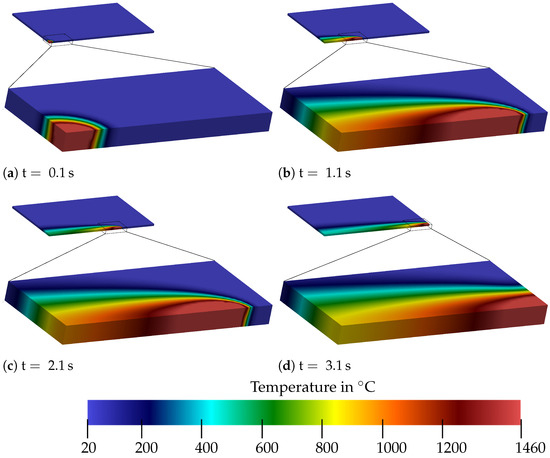
Figure 20. Perspective view of the temperature distribution for different time points of the calculation. Shown is the complete BVP with a respective section of the size $12\mathrm{mm}\times 7\mathrm{mm}\times 2.2\mathrm{mm}$.

Comparison of Finite-Element Results to Experimental Data and CFD Simulations

In the following, the simulation results from the FE analysis using the volumetric heat source and the Lamé curves are compared with the results from the CFD analysis and the experiments. Therefore, the temperature data from specific points within the domain in association with the thermocouples is analyzed in detail. For the comparison with the Lamé curve model based on moving Dirichlet boundary conditions, an additional simulation was carried out using the same mesh and the same time step size as for the simulation with the new heat source model. For further information on the simulation with Lamé curves, please refer to [22]. Furthermore, a comparison of the cross-section of the weld seam with the CFD and experimental data in relation to Figure 5 was carried out.

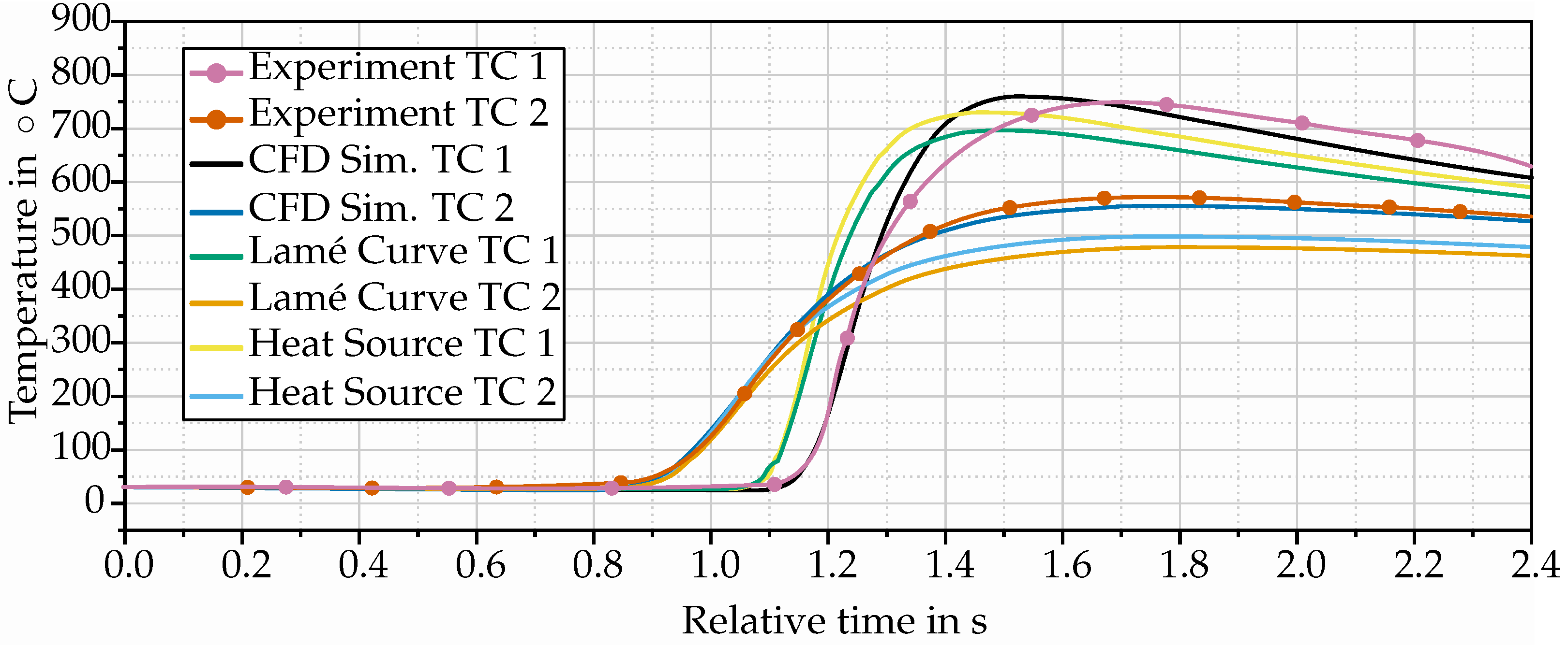
First, the resulting temperature curves (see Figure 21) were evaluated at the locations where the thermocouples were attached in the experiment. These were located on the surface at positions TC 1 $(30\mathrm{mm},2.1\mathrm{mm},0\mathrm{mm})$ and TC 2 $(25\mathrm{mm},3.2\mathrm{mm},0\mathrm{mm})$; see Figure 22. Although a time scale along the x-axis is indicated in Figure 21, no exact time points have been added to the axis. The reason for this is that the experiments required a certain amount of time before the laser started to advance. However, the exact time at which the laser started to run is unknown, which is why it was decided to align the curves over the temperature rise of TC 2, as this was the first relevant time point. Nevertheless, the time scale was roughly represented as an x-axis in order to be able to read off the theoretical time sequence. The distance between two continuous vertical lines corresponds to $0.2$ s. This means that the temperature is shown over a complete period of $2.4$ s. Also note that the markers on the lines of experimental measurements do not correspond to explicit measuring points, but are used to let the experimental curves stand out among the simulated data.

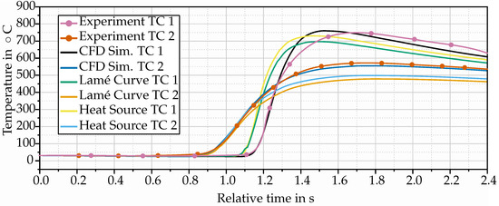
Figure 21. Resulting temperature curves over relative time of the thermocouples from the FE simulations and the CFD simulation at the locations of the thermocouples from the experiment. The curves of the various methods were aligned with the rise in temperature of TC 2 from the experiment.

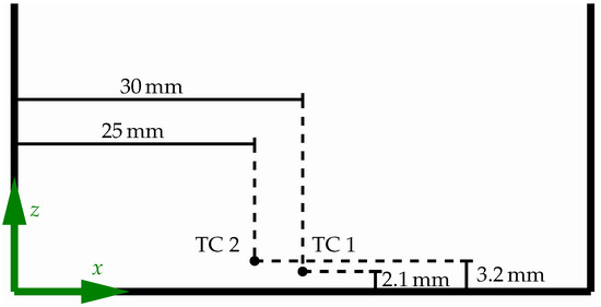
Figure 22. Location of the thermocouples.

Comparing the curves, it is noticeable that the temperatures from the FEM simulations were generally lower than those from the CFD simulation and the experiment. For thermocouple TC 1, the difference of the maximum temperature compared to the CFD simulations and the experiment was around 20–30 $°\mathrm{C}$. Meanwhile, the maximum temperature of the first thermocouple for the Lamé curves was 40–60 $°\mathrm{C}$ below the maximum temperature of TC 1. The behavior compared to the second thermocouple was similar. The maximum temperature from the CFD simulation and experiment was around 50–60 $°\mathrm{C}$ above the maximum temperature of the volumetric heat source model. The Lamé curves, on the other hand, only showed a temperature of around $480°\mathrm{C}$ and were 70–80 $°\mathrm{C}$ below the maximum temperature of TC 2. Nevertheless, it is noticeable that only the maximum temperatures differed and a similar behavior in temperature increase and cooling was observed for all cases. When the temperature rise was compared, it was similar for all four data sets for the first and second thermocouple. This means that with the beginning of the temperature rise, $0.3$ s up to $0.4$ s passed until the maximum temperature of TC 1 was reached. Only the temperature rise for the experiment was somewhat slower. This was followed by a cooling of around 150 $°\mathrm{C}$ within the next $0.7$ s to $0.9$ s for the CFD simulation and the experiment, while the temperatures for the heat source and the Lamé curves cooled down by around 120 $°\mathrm{C}$ within $0.8$ s and $1.0$ s. The behavior of TC 2 was also similar. The rise of the temperature to its maximum occurred within about $0.9$ s. Afterwards, a cooling occurred, but it was significantly weaker than for TC 1. In general, it can be said that the qualitative behavior of the three methods was very close to the experiment, and thus, all simulations were able to describe the experiments well. For further information on the thermal behavior, additional points were evaluated for the FE simulation with regard to their temperature profile. These points were at the same distance from the weld seam as the thermocouples, but varied in position along the x-axis. The evaluation showed that the temperature curves were congruent, and thus, a steady state was established after a certain distance from the starting point. One thing that stood out, despite the qualitatively similar progression of individual curves, was that the temperature of the FE simulation rose earlier than those from the CFD simulation or the experiment. This behavior may be due to minor inaccuracies when measuring the distances between the thermocouples TC 1 and TC 2 or the distance to the weld seam. Another reason could be the heat conduction in the system. In the implemented material model, Fourier’s law was taken into account.

In a second comparison, the cross-sections of the FE analysis were compared with those of the CFD simulation and the experiments; see Figure 23. The figure shows the isotherms of the CFD simulation on the left and the isotherms of the FE simulation with the volumetric heat source on the right. In the background is the cross-section of the experiment, with the fusion line shown in white. The black lines represent the isotherms from inside to outside. This means that the innermost black line is the isotherm of the liquidus temperature ($1460°\mathrm{C}$), the second innermost line is the isotherm for a temperature of $1400°\mathrm{C}$, and then, the isotherms follow in descending steps of 100-degree intervals, in other words for $1300°\mathrm{C}$, $1200°\mathrm{C}$, and so on.

Figure 23. Comparison of the temperature profiles: The white line indicates the fusion line as identified from the experimental data (cross-section). In comparison, the left side shows the temperature profile resulting from the CFD simulation, while the right side shows the temperature profile of the FE simulation with the physically based heat source model.

It is noticeable that, for the CFD simulation, the fusion line in the lower part is congruent with the liquidus isotherm, and in the upper part, the liquidus isotherm is slightly inside the fusion line. For the volumetric heat source, on the other hand, the liquidus isotherm lies completely inside the fusion line. On the other hand, the isotherm for $1400°\mathrm{C}$ approximately maps the fusion line. The difference in heat distribution was already noticeable in the first comparison due to the lower maximum temperatures at the thermocouples. This may be due to the same reason that heat conduction is realized differently in CFD simulation and FE simulation and needs to be further investigated in the future.

6. Summary and Discussion

In this paper, we have presented a new heat source model for laser beam welding. We discuss the experimental background of the laser beam welding process in Section 2. Section 3 gives an overview on the simulation of the laser beam welding process using a FEM scheme and gives insight into the CFD model.

The CFD results of the computed melting isotherm form the basis for our heat source model, which is described in detail in Section 4. There, we have presented a new physics-based heat source model based on the definition of a heat source term inside the melting pool for welding simulations. The key difference from existing models, such as Goldak (see [11]), is that we did not describe the laser directly, but we aim for a description of a constant temperature at the level of the melting temperature in the melting pool. This is reasonable when we want to analyze the surrounding region of the melt pool to identify, e.g., the mushy zone or the heat-affected zone in general. Complex physical effects, such as ray reflecting and evaporation, taking place in the melt were not considered in the heat source model directly, but entered indirectly by using data from CFD simulation including such effects. In CFD simulations, these complex physical phenomena can be more easily realized compared to structural FEM simulations, where they would pose high difficulties. With a similar aim, a Lamé curve model with moving Dirichlet boundary conditions was realized in [37]; however, moving Dirichlet boundary conditions may be hard to realize in some cases. Both models rely on a prior identification of a melting isotherm, for example based on CFD simulations.

The heat source model achieved a constant temperature inside the melting pool by modification of the power density input at each Gaussian point. Based on the given power of the laser beam, a maximal power density was calculated, which acted as an upper limit. While in the heating phase, every point received the identical power density input related to the maximal value, as long as the liquidus temperature was not achieved. The power density was modified as soon as an estimation of the current temperature exceeded the liquidus temperature. Then, the power density was reduced to avoid overshooting of the temperature in the melting pool and possible fluctuation of the temperature. The power density, furthermore, was set to zero when the Gaussian point had exceeded the liquidus temperature in the previous time step. In addition to this modification of the power density at each Gaussian point depending on the local temperature, a redistribution of unused energy was considered. When some points in the melting pool received a lower energy input than the maximal value, the remaining energy was redistributed to a point where the liquidus temperature had not been achieved yet. This was performed in an averaged sense by calculating a factor, which was then multiplied with the maximal power density. A limit factor has been implemented to prevent fluctuations. The comparison in Section 5 shows that this redistribution increases the accuracy with which the prescribed isotherm is achieved in the simulation.

We conducted two laser beam welding simulations using the presented heat source model. First, a steady conical heat source model was analyzed, using a simplified, artificial isotherm and considering no movement of the laser beam. In this convergence study, we analyzed the sensitivity of the model with respect to discretization in space and time. It became clear that, with a suitable discretization, we were able to describe the prescribed isotherm accurately. Furthermore, the influence of the redistribution of the power density in the melt pool was analyzed. Section 5.3 then presents a boundary-value problem for a moving heat source, where an FEM model with a varying element size was used. Therein, the realistic isotherm obtained from the prior CFD simulation served as the input for the welding process. The resulting temperature distribution in the welded part was discussed, where the typical elongated tail of the heated material was found in the rear of the melt pool. Furthermore, we compared the results to experimental data obtained from thermocouples, which were placed at two positions close to the weld seam. A very good agreement was found in the characteristics of the temperature curves, showing only minor differences of 4%. Finally, a cross-section of the weld was analyzed, showing the approximation of the experimental fusion line.

The heat source model will be used in our future studies to identify the mushy zone in the welded part in order to perform further analyses in this region in view of solidification cracking.

References

- Dilthey, U. Schweißtechnische Fertigungsverfahren 1: Schweiß- und Schneidtechnologien, 3rd ed.; VDI-Buch; Springer: Berlin/Heidelberg, Germany, 2006. [Google Scholar]
- Hills, R.N.; Loper, D.E.; Roberts, P.H. A thermodynamically consistent model of a mushy zone. Q. J. Mech. Appl. Math. 1983, 36, 505–540. [Google Scholar] [CrossRef]
- Yoshioka, H.; Tada, Y.; Hayashi, Y. Crystal growth and its morphology in the mushy zone. Acta Mater. 2004, 52, 1515–1523. [Google Scholar] [CrossRef]
- Rosenthal, D. The theory of moving sources of heat and its application to metal treatments. Trans. Am. Soc. Mech. Eng. 1946, 68, 849–865. [Google Scholar] [CrossRef]
- Boulton, N.; Martin, H.L. Residual stresses in arc-welded plates. Proc. Inst. Mech. Eng. 1936, 133, 295–347. [Google Scholar] [CrossRef]
- Bruce, W. The thermal distribution and temperature gradient in the arc welding of oil well casing. J. Appl. Phys. 1939, 10, 578–584. [Google Scholar] [CrossRef]
- Mahla, E.M. Heat Flow in Arc Welding. Ph.D. Thesis, Lehigh University, Bethlehem, PA, USA, 1941. [Google Scholar]
- Eagar, T.; Tsai, N. Temperature fields produced by traveling distributed heat sources. Weld. J. 1983, 62, 346–355. [Google Scholar]
- Pavelic, V.; Tanbakuchi, R.; Uyehara, O.; Myers, P. Experimental and computed temperature histories in gas tungsten arc welding of thin plates. Weld. J. Res. Suppl. 1969, 48, 296–305. [Google Scholar]
- Wu, C.; Wang, H.; Zhang, Y. A New Heat Source Model for Keyhole Plasma Arc Welding in FEM Analysis of the Temperature Profile. Weld. J. 2006, 85, 284. [Google Scholar]
- Goldak, J.; Chakravarti, A.; Bibby, M. A new finite element model for welding heat sources. Metall. Trans. B 1984, 15, 299–305. [Google Scholar] [CrossRef]
- Rahman Chukkan, J.; Vasudevan, M.; Muthukumaran, S.; Ravi Kumar, R.; Chandrasekhar, N. Simulation of laser butt welding of AISI 316L stainless steel sheet using various heat sources and experimental validation. J. Mater. Process. Technol. 2015, 219, 48–59. [Google Scholar] [CrossRef]
- Farias, R.; Teixeira, P.; Vilarinho, L. Variable profile heat source models for numerical simulations of arc welding processes. Int. J. Therm. Sci. 2022, 179, 107593. [Google Scholar] [CrossRef]
- Winczek, J. The influence of the heat source model selection on mapping of heat affected zones during surfacing by welding. J. Appl. Math. Comput. Mech. 2016, 15, 167–178. [Google Scholar] [CrossRef]
- Heinze, C.; Schwenk, C.; Rethmeier, M. Effect of heat source configuration on the result quality of numerical calculation of welding-induced distortion. Simul. Model. Pract. Theory 2012, 20, 112–123. [Google Scholar] [CrossRef]
- Beygi, R.; Marques, E.; da Silva, L.F. Computational Concepts in Simulation of Welding Processes; Springer: Cham, Switzerland, 2022. [Google Scholar]
- Lazov, L.; Teirumnieks, E.; Draganov, I.; Angelov, N. Numerical modeling and simulation for laser beam welding of ultrafine-grained aluminium. Laser Phys. 2021, 31, 066001. [Google Scholar] [CrossRef]
- Fan, X.; Qin, G.; Jiang, Z.; Wang, H. Comparative analysis between the laser beam welding and low current pulsed GMA assisted high-power laser welding by numerical simulation. J. Mater. Res. Technol. 2023, 22, 2549–2565. [Google Scholar] [CrossRef]
- Duggirala, A.; Kalvettukaran, P.; Acherjee, B.; Mitra, S. Numerical simulation of the temperature field, weld profile, and weld pool dynamics in laser welding of aluminium alloy. Optik 2021, 247, 167990. [Google Scholar] [CrossRef]
- Yan, S.; Meng, Z.; Chen, B.; Tan, C.; Song, X.; Wang, G. Prediction of temperature field and residual stress of oscillation laser welding of 316LN stainless steel. Opt. Laser Technol. 2022, 145, 107493. [Google Scholar] [CrossRef]
- de Oliveira, A.F.M.; Magalhães, E.d.S.; Paes, L.E.d.S.; Pereira, M.; da Silva, L.R. A Thermal Analysis of LASER Beam Welding Using Statistical Approaches. Processes 2023, 11, 2023. [Google Scholar] [CrossRef]
- Artinov, A.; Karkhin, V.; Bakir, N.; Meng, X.; Bachmann, M.; Gumenyuk, A.; Rethmeier, M. Lamé curve approximation for the assessment of the 3D temperature distribution in keyhole mode welding processes. J. Laser Appl. 2020, 32, 022042. [Google Scholar] [CrossRef]
- Artinov, A.; Bachmann, M.; Rethmeier, M. Equivalent heat source approach in a 3D transient heat transfer simulation of full-penetration high power laser beam welding of thick metal plates. Int. J. Heat Mass Transf. 2018, 122, 1003–1013. [Google Scholar] [CrossRef]
- Hildebrand, J. Numerische Schweißsimulation-Bestimmung von Temperatur, Gefüge und Eigenspannung an Schweißverbindungen aus Stahl-und Glaswerkstoffen. Ph.D. Thesis, Bauhaus-Universität Weimar, Weimar, Germany, 2008. [Google Scholar]
- Sahoo, P.; Debroy, T.; McNallan, M. Surface tension of binary metal—Surface active solute systems under conditions relevant to welding metallurgy. Metall. Trans. B 1988, 19, 483–491. [Google Scholar] [CrossRef]
- Simo, J.; Miehe, C. Associative coupled thermoplasticity at finite strains: Formulation, numerical analysis and implementation. Comput. Methods Appl. Mech. Eng. 1992, 98, 41–104. [Google Scholar] [CrossRef]
- Wriggers, P. Nonlinear Finite Element Methods; Springer Nature: Berlin/Heidelberg, Germany, 2008. [Google Scholar]
- Knothe, K.; Wessels, H. Finite Elemente: Eine Einführung für Ingenieure, 5th ed.; Springer: Berlin/Heidelberg, Germany, 2017. [Google Scholar]
- Zain-Ul-Abdein, M.; Nélias, D.; Jullien, J.; Deloison, D. Thermo-mechanical Analysis of Laser Beam Welding of Thin Plate with Complex Boundary Conditions. Int. J. Mater. Form. 2008, 1, 1063–1066. [Google Scholar] [CrossRef]
- Agarwal, G.; Gao, H.; Amirthalingam, M.; Hermans, M. Study of Solidification Cracking Susceptibility during Laser Welding in an Advanced High Strength Automotive Steel. Metals 2018, 8, 673. [Google Scholar] [CrossRef]
- Kik, T. Computational Techniques in Numerical Simulations of Arc and Laser Welding Processes. Materials 2020, 13, 608. [Google Scholar] [CrossRef] [PubMed]
- Kik, T. Heat Source Models in Numerical Simulations of Laser Welding. Materials 2020, 13, 2653. [Google Scholar] [CrossRef] [PubMed]
- Taylor, R. FEAP—A Finite Element Analysis Program, Version 8.2. Department of Civil and Environmental Engineering, University of California at Berkley, Berkley, California 94720-1710, March 2008. Available online: http://projects.ce.berkeley.edu/feap/ (accessed on 18 March 2024).
- Sente Software Ltd. JMatPro; Sente Software Ltd.: Guildford, UK, 2022. [Google Scholar]
- Richter, F. Die physikalischen Eigenschaften der Stähle—Das 100 Stähle-Programm; Technical Report; TU Graz: Styria, Austria, 2011. [Google Scholar]
- Geuzaine, C.; Remacle, J.-F. Gmsh: A 3-D finite element mesh generator with built-in pre- and post-processing facilities. Int. J. Numer. Methods Eng. 2009, 79, 1309–1331. [Google Scholar] [CrossRef]
- Bakir, N.; Artinov, A.; Gumenyuk, A.; Bachmann, M.; Rethmeier, M. Numerical simulation on the origin of solidification cracking in laser welded thick-walled structures. Metals 2018, 8, 406. [Google Scholar] [CrossRef]
Disclaimer/Publisher’s Note: The statements, opinions and data contained in all publications are solely those of the individual author(s) and contributor(s) and not of MDPI and/or the editor(s). MDPI and/or the editor(s) disclaim responsibility for any injury to people or property resulting from any ideas, methods, instructions or products referred to in the content. |
© 2024 by the authors. Licensee MDPI, Basel, Switzerland. This article is an open access article distributed under the terms and conditions of the Creative Commons Attribution (CC BY) license (https://creativecommons.org/licenses/by/4.0/).