Abstract
The superconducting transition temperature, , can be calculated for practically all superconducting elements using the Roeser–Huber formalism. Superconductivity is treated as a resonance effect between the charge carrier wave, i.e., the Cooper pairs, and a characteristic distance, x, in the crystal structure. To calculate for element superconductors, only x and information on the electronic configuration is required. Here, we lay out the principles to find the characteristic lengths, which may require us to sum up the results stemming from several possible paths in the case of more complicated crystal structures. In this way, we establish a non-trivial relation between superconductivity and the respective crystal structure. The model enables a detailed study of polymorphic elements showing superconductivity in different types of crystal structures like Hg or La, or the calculation of under applied pressure. Using the Roeser–Huber approach, the structure-dependent different ’s of practically all superconducting elements can nicely be reproduced, demonstrating the usefulness of this approach offering an easy and relatively simple calculation procedure, which can be straightforwardly incorporated in machine-learning approaches.
1. Introduction
We use the Roeser–Huber formalism [1,2,3,4] to calculate the superconducting transition temperature, , of the superconducting elements in ambient conditions as well as under pressure. Up to now, there are 53 superconducting elements known (in ambient conditions and under pressure, [5,6]), and three more are superconductors under special conditions (i.e., in thin film form (Cr), after irradiation (Pd), or C in several modifications [7], e.g., diamond films, alkali-doped fullerene, and carbon nanotubes). A periodic table of the elements with the -data from the literature is presented in Figure 1. From all reviews and teaching books covering this field [6,7,8,9,10,11,12,13], it is clear that there is no simple relation between and the respective crystal structure. Moreover, some elements are polymorphic superconductors with different crystal structures, e.g., La, Hg and Ga, and some elements show changes of the crystal structure under pressure (e.g., Fe becomes superconducting under pressure in the non-magnetic phase (hexgonally close-packed (hcp) -Fe phase) [14,15,16]). Commonly, bandstructure calculations are performed to obtain requiring many parameters (see, e.g., Refs. [17,18]) and using given crystal structures as a base, which is, however, not straightforward to enable comparison of a large variety of elements and different crystal structures. Thus, a relatively simple calculation procedure like the Roeser–Huber formalism, which requires only knowledge of the crystal structure and the basic electronic configuration with no free parameters, has clear advantages when being incorporated as a test in machine learning approaches to find new superconducting materials [19,20,21], because there is only a limited number of crystal structures to be considered.
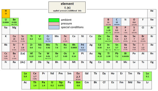
Figure 1.
Superconducting elements in the periodic table ( = superconductor in ambient conditions,
  = superconductor under applied pressure, and
  = superconductor with special conditions). Given are the abbreviations of the names, the transition temperatures, , and the applied pressure or some extra info for each element. Hydrogen H is marked in orange concerning the prediction to be a room-temperature superconductor under high pressure. All data given are taken from Refs. [6,7,8,9,10,11,12,13].
= superconductor in ambient conditions, = superconductor under applied pressure, and = superconductor with special conditions). Given are the abbreviations of the names, the transition temperatures, , and the applied pressure or some extra info for each element. Hydrogen H is marked in orange concerning the prediction to be a room-temperature superconductor under high pressure. All data given are taken from Refs. [6,7,8,9,10,11,12,13].
2. Principles of the Model
The basic idea of the Roeser–Huber formalism is the view of superconductivity being a resonance effect between the charge carrier wave (Cooper pairs with the de Broglie wavelength, ) moving through the crystal lattice and a characteristic distance, x, within the crystal unit cell. Interpreting the superconducting transition in a resistance measurement of a superconductor as an integrated resonance curve helps to visualize this resonance effect. The resistance data reflect the material properties and the microstructure (e.g., grain boundaries), but the superconducting transition itself is only due to the Cooper pairs. Of course, their underlying properties are influenced by the band structure configuration of the material. As discussed in Refs. [22,23], the mass of the Cooper pairs is given by with being the free electron mass. The characteristic distance, x, which can be deduced from the crystal unit cell as an interatomic distance being different for various possible directions, and some knowledge about the electronic structure of the material are sufficient to calculate , based on the particle-in-box (PiB) principle [24]. As described already in Refs. [3,25], the Roeser–Huber formula is given as
with describing the lowest level energy of the PiB. h denotes the Planck constant, the Boltzmann constant, is a parameter with the unit of a mass, and the sum is taken for all possible directions, , as explained below. For all unit cells of metallic elemental superconductors, there are no 2D-like superconducting planes, thus (describing the number of superconducting planes of 2D superconductors) is set to 1. The interatomic distance x now depends on each crystallographic direction (which will be called superconducting path hereafter), , and the two correction factors, and , the determination of which is discussed below.
Following the work of Moritz [25], there are four important points to be considered when calculating for metallic elements:
- (i)
- The distance x corresponds to an interatomic distance similar to the PiB approach applied in [1]. The distance x is obtained from possible symmetric paths (also called superconducting directions in the following) for the movement of the charge carrier wave within the crystal structure, as discussed below. The crystallographic data come from respective databases [26,27], which is an important issue for application of the Roeser–Huber formalism in machine-learning calculation approaches.
- (ii)
- The parameter for high- superconductor (HTSc) compounds was taken as 2. For element superconductors, is much higher as all the phononic interactions (Fermi temperature, Debye temperature, effective mass, charge carrier density) are incorporated in the parameter . In a first approximation, 1900, which corresponds closely to the mass of a proton ( 1836.15). Regarding the location of metallic superconductors in a Uemura plot ( as function of the Fermi temperature, [28,29] and denoting the Fermi velocity, m* is the effective mass) in the lower right corner with 10… 10 K, the high value for is reasonable. This significant difference between elemental metallic superconductors and the HTSc materials was also pointed out by Emery and Kievelson [30] mentioning the substantial phase rigidity of the superconducting state in, e.g., lead at all temperatures below .
- (iii)
- A first correction factor is required to account for more complex crystal structures. Atoms being close to a superconducting direction may have an influence on the moving charge carriers via the phonon interaction. Therefore, the number of atoms passed within a unit cell is counted. This correction was originally added to the parameter via:which we keep here for consistency. Regarding the definition of given above, the relation is thus incorporated in . Here, represents the number of the charge carriers and denotes the number of the near, passed atoms along each superconducting path. A correction factor can be then defined as . In case there are no (near) passed atoms, then 1.As the symmetry of the superconducting path plays an important role for our considerations, the passed atoms must be symmetrically arranged along the superconducting path, as otherwise the charge carriers would be not in phase due to the unsymmetric forces. This implies that superconductivity cannot exist in directions with unsymmetrically arranged passed atoms. As test for the influence of the passed atoms, we define a relation , with l being a distance perpendicular to the direction of the moving charge carriers. If 0.5, the passed atoms show an influence on the superconductivity and must be counted in . Here, it is important to point out that and are not free parameters, but are given from the respective crystal structure being investigated. A special case for determining will be encountered for hcp Fe under pressure as discussed below.
- (iv)
- A second correction factor is necessary to account for anisotropic superconductivity, which can even lead to so-called multimode superconductivity. The factor gives a relation between the specific directions for the charge carrier wave, , in the given crystal structure. The energy and the transition temperature are then calculated for each existing superconducting path , and the results must be summed up according to Equation (1). If one of the directions gives a reasonable value for to compare with the experimentally determined , this direction is taken as the superconducting path. However, the -values of the other directions and the complete sum of all may also have important implications as, e.g., in the case of Al, which was discussed in Ref. [3], the experimental value of is reached with 2 of the possible 4 directions in the fcc structure, but the total sum of all 4 directions is strikingly close to the increased , when measuring thin films. A similar situation is given for the energies, . may be compared to the pairing energy or energy gap as determined experimentally. Thus, all - and -values must be calculated for a given material. For most elemental superconductors, 1, in contrast to the metallic alloys NbSn or MgB, where superconducting directions can exist several times within one unit cell, as already discussed in Ref. [3].
The Roeser–Huber formalism (1) does not contain any free parameters, as all the required inputs are given via the crystal unit cell (i.e., x and ) and from the basic electronic configuration of the material. It must be noted here that the Roeser–Huber formalism does not describe how the Cooper pairs are formed, and so it is not possible to determine if a given material is a superconductor. However, regarding the limits of the parameter ( 2, and is set by the demand of the BCS-theory that the effective charge carrier mass, cannot be smaller than for isotropic, spherical Fermi surfaces [31]), one may deduce a possibility to judge if superconductivity for a given material and crystal structure exists. This will be elaborated in future works.
3. Results and Discussion
Figure 1 presents the periodic table of the superconducting elements. Thirty-three of them are superconductors in ambient conditions with the reported -values ranging between 0.00053 K (Bi) to 9.2 K (Nb). Under applied high pressures, 20 more elements become superconductors, and the -values can be as high as 20 K (Li), and also several non-metals (O, P, S, Br, I) were found to supercoduct as well. Finally, three elements (C, Cr and Pd) are superconductors in ambient conditions, but only under special conditions—C in several modifications (alkali-doped C, carbon nanotubes, diamond) having also different values of , Cr only as thin film material and Pd only after irradiation with He+-ions [32].
In Figure 2a, is plotted versus the year of discovery. Up to 1950, only superconductors at ambient conditions were known. In 1970, the measured of La under pressure exceeded the first time the ambient of Nb, and after the discovery of the HTSc materials, the high-pressure experiments were extended to find elements with even much higher -values up to 20 K (Li). Figure 2b presents a logarithmic plot of in relation to the respective crystal structure (body-centered cubic (bcc), face-centered cubic (fcc), hexagonally close-packed (hcp), tetragonal (tetra), monoclinic (mono), orthorhombic (ortho), fcc* and double hexagonally close-packed (dhcp)), and it is obvious that there is no direct and simple relation between and the crystal structures. For example, the highest is obtained for bcc Nb, but bcc Li shows the second-lowest at ambient conditions. Figure 2b indicates that similar behavior holds for all other crystal lattice types as well. Thus, the link between crystal structure and , if existing, must be a much more subtle and non-trivial one.
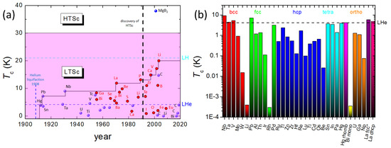
Figure 2.
(a) as a function of the year of discovery of the superconducting elements (•—ambient conditions, •—under pressure). Note the highest of all elements at 20 K for Li under pressure. The borderlines for liquid He (LHe) and liquid H (LH) are also presented. The 30 K-line marks the border between LTSc and HTSc materials, crossed by the alloy superconductor MgB2, which is given for comparison. (b) Logarithmic plot of of various elements in ambient conditions with respect to their crystal structure (body-centered cubic (bcc), face-centered cubic (fcc), hexagonally close-packed (hcp), tetragonal (tetra), monoclinic (mono), orthorhombic (ortho), fcc* and double hexagonally close-packed (dhcp)). The highest in ambient conditions is obtained for Nb with bcc structure, the lowest to date has Bi with a monoclinic structure.
Exactly this task is fulfilled by the Roeser–Huber formalism, establishing a non-trivial relation between and the given crystal structures. For a successful application of the Roeser–Huber formalism, one needs the information of the possible crystal structures, and about the electronic configuration to count (similar to the valence electron count used by Matthias [9]) and the number of passed (or near) atoms, (as determined from the given crystal structure using the relation 0.5.
In Ref. [2], of the elements Nb, V, Ta (bcc) and Hg (rhombohedral) were calculated introducing the procedure. In [3], the calculation of Pb and Al (fcc) and Sn (tetragonal) was presented. As an example, here the two most interesting cases of the polymorphic elements La and Hg will be discussed, where two different crystal structures exist with different -values.
Figure 3 presents all the crystal structures, which need to be calculated for this purpose. For -Hg, the details of the crystal structure and the calculation steps were already presented in Ref. [2]. The structure is rhombohedral, being a simple cubic cell with the angles 70.52. -Hg is tetragonal, and more precisely, tetragonal bcc with and having an atom in the center of the unit cell. The crystal structure fcc* is unique to the rare earth elements La, Ce and Yb [33]. Indeed, in the [111]-direction, the structure is similar to the standard fcc one, only the number of atoms involved is different. The dhcp-structure is the common one for most of the rare earth elements, and is treated here the first time. Both fcc* and dhcp structures are derivatives of the hcp structure as indicated with letters A–C.
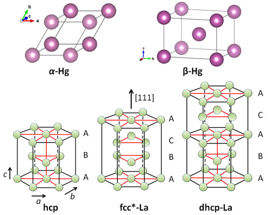
Figure 3.
Upper row: Crystal structures of -Hg (rhombohedral) and -Hg (tetragonal bcc). Lower row: (left) hcp-crystal structure (e.g., -Fe) and the ones of the rare-earth element La, fcc* (middle) and dhcp (right). These structures were redrawn from Ref. [33].
The case of the rhombohedral Hg (-Hg) is simple. All distances between the atoms correspond to a, and all 3 rhombohedral directions are equal. There is only one possible superconducting path along a, which fulfills the symmetry condition. The calculation yields one value for 4.175 K, which corresponds well to the tabulated of 4.15 K [7]. In the case of the tetragonal Hg (-Hg) [34], there are three possible superconducting paths like in the standard bcc structure, each with an own energy and .
- (1)
- along the space diagonal via the central atom. Thus, x is the half of this distance, so and 1.
- (2)
- corresponds to the crystal edge along a, so and 1.
- (3)
- along the diagonal in the top/bottom plane with and 4, i.e., the other two atoms in this plane and the central atoms (one of the given cell and the one of the cell below) are close enough to have an influence on the superconducting path.
See also the Supplementary Material for drawings of each superconducting direction. Table 1 presents the details of the superconducting paths fulfilling the symmetry condition together with the calculations performed.

Table 1.
The crystal parameters a and c, the direction number, the distance x, , , , the calculated energies and the calculated for Hg (rhombohedral -Hg and tetragonal bcc -Hg) and La (fcc* and dhcp).
Here, one can see that direction (1) yields 3.792 K, which again fits closely to the tabulated value of 3.95 K [7]. For the comparison of the calculated and the experimental -values, one must note that the Roeser–Huber approach requires (the mean-field corresponding to the maximum of the derivative dR/dT). This is not always the case concerning various literature data, where often or 50 % of the normal-state resistivity are given as . Therefore, the small deviations obtained may stem from this problem.
In the case of La, there are two crystal structures which are both unique to the rare-earth materials, fcc* and double hexagonally close-packed (dhcp) [33]. Figure 3 shows that for both structures, the hexagonal top and bottom layers labeled A are the same like in the hcp structure. In fcc*, there are more atoms as in the conventional fcc structure, but some of the possible superconducting paths are basically the same, except that we have to account for the near atoms. Therefore, both systems have three possible paths for superconductivity, which fulfill the condition of symmetry. For dhcp La, the superconducting paths are:
- (1)
- Along the c-axis in the center of the structure with , and counts to 3.
- (2)
- Oriented along the edge with (1), and
- (3)
- In the plane between 2 not neighboring atoms with and 2.
For fcc* La, paths (2) and (3) are the same as before, and path (1) takes the length with 6. Table 1 gives the results of the calculations.
The experimental of dhcp La is 4.8 K, and of the fcc*-La is 6 K [6,8]. Looking at Table 1 reveals that we must combine at least two directions to reach the experimental value, e.g., (1) + (3) or (2) + (3) for dhcp with (1) + (3) yielding 4.85 K, and for fcc *, even all three directions must contribute to reach the experimental value with the sum yielding 6.245 K. Given the large experimental variation of reported [8], this is again a perfect coincidence.
As an example for an element being superconducting under applied pressure, we have chosen the hcp -Fe, which is nonmagnetic [15]. Therefore, superconductivity may develop in this specific crystal structure. The properties of hcp Fe were discussed in the work by Roth [16], using all available information from the literature. To obtain reasonable values for comparison with the experimentally measured -values, it is important that also the crystallographic data under pressure are available. For hcp iron, one can find two equations describing the lattice parameters under pressure, determined using x-ray diffraction techniques [35]:
and
Using Equations (3) and (4), one can determine the proper crystal parameters at the given applied pressure. Following Shimizu et al. [14], the maximum of 2 K is reached at a pressure of 21 GPa. Fe has the electron configuration [Ar] 3d6 4s2, so in total 8 electrons in the outer shell. Fe can have oxidation states from −2 to 7. As Fe also has a specific resistance below 10−8 Ωm, it is reasonable to consider all eight outer electrons like in the e/a-count by Matthias [9] being involved in superconductivity. The hcp structure (see Figure 3) has basically the same superconducting paths as the dhcp structure discussed before, that is,
- (1)
- Along the c-axis in the center of the structure with , and 3.
- (2)
- Oriented along the edge with (1), and
- (3)
- In the top/bottom plane between two not-neighboring atoms with and 2.
With this information, can now be calculated as summarized in Table 2.
Table 2.
The crystal parameters a and c, the direction number, the distance x, , , , the calculated energies and the calculated for -Fe under a pressure of 21 GPa [14] and 22.2 GPa [36].
Now, we have to realize that the value for of 2 K reported is the onset temperature of superconductivity, and the transition width is quite broad [14], so is much smaller, possibly between 1.5 and 1.7 K, as the full resistance curve at 21 GPa is not published in [14]. In [36], the high-pressure experiments on Fe were repeated and the highest with 2.5 K was obtained at 22.2 GPa. Here, the complete resistance curve is published showing a broad superconducting transition with 1.5 K, yielding 1.64 K. Thus, the calculated values of direction (1) or (2) give a good representation of the situation with only a small error margin. To summarize this, it is possible to calculate the of elements under pressure using the Roeser–Huber formalism, provided that experimental crystallographic data are available.
Finally, Figure 4 presents the Roeser–Huber plot with many calculated superconducting materials, high- superconductors (HTSc, marked with a red circle), metallic alloys (blue circle) and elements (green circle). Practically all superconducting elements can be calculated using the Roeser–Huber formalism with only small error margins. The only exceptions are the very low- materials Li, Be and Bi, where the low values of can only be reproduced with an adaptation of , which is due to either an extremely small charge carrier mass (Li, Be) or a large electron mean free path (Bi). In contrast, the Roeser–Huber formalism works well to calculate the respective -values of the same materials under applied pressure. A very important point is here that all the data of obtained fall on a common, straight line (blue), which follows the equation for a particle in a box [24] with the slope 5.061 × 10 m kg K. This result enables the Roeser–Huber formalism to act as a test for given predictions of , e.g., for the case of metallic hydrogen as was done recently in Ref. [37].
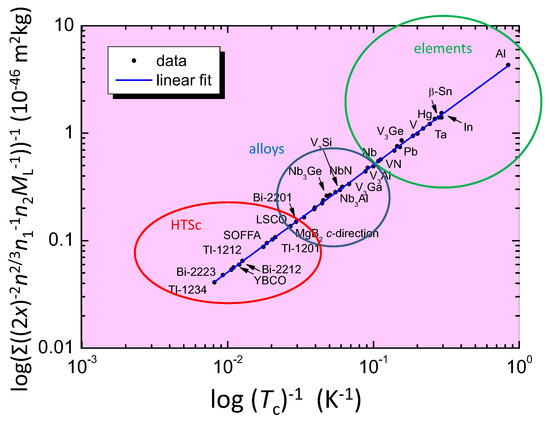
Figure 4.
The Roeser–Huber plot for a large number of superconducting materials. Red circle: HTSc, blue circle: alloys, and green circle: elemental superconductors. Some overlaps between these regions do exist. For clarity, only some of our collected data are included.
4. Conclusions
To conclude, we have presented -calculations of two polymorphic superconducting elements (Hg, La) using the Roeser–Huber formalism and for -Fe (hcp) under pressure. The principles of this formalism enable to reproduce the different -values of various crystal structures of the same elements, which directly proofs the validity of the concept. This will enable us to apply this formalism for the prediction of of still unknown superconducting materials, e.g., in machine learning approaches.
Supplementary Materials
The following are available online at https://www.mdpi.com/article/10.3390/met12020337/s1, Figure S1: Crystal structure of -Hg (rhombohedral) and superconducting direction, Figure S2: Crystal structure of -Hg (tetragonal bcc) and superconducting directions (1)–(3), Figure S3: Crystal structure hcp and superconducting directions (1)–(3), Figure S4: Crystal structure fcc* and superconducting directions (1)–(3), Figure S5: Crystal structure dhcp and superconducting directions (1)–(3).
Author Contributions
Conceptualization, M.R.K.; formal analysis, A.K.-V. and M.R.K.; investigation, A.K.-V. and M.R.K.; visualization, A.K.-V. and M.R.K., writing—original draft preparation, M.R.K.; writing—review and editing, A.K.-V. and M.R.K. All authors have read and agreed to the published version of the manuscript.
Funding
This work is part of the SUPERFOAM international project funded by ANR and DFG under the references ANR-17-CE05-0030 and DFG-ANR Ko2323-10, respectively.
Institutional Review Board Statement
Not applicable.
Informed Consent Statement
Not applicable.
Data Availability Statement
Data are available from the authors upon reasonable request.
Conflicts of Interest
The authors declare no conflict of interest.
References
- Roeser, H.P.; Hetfleisch, F.; Huber, F.M.; Stepper, M.; von Schoenermark, M.F.; Moritz, A.; Nikoghosyan, A.S. A link between critical transition temperature and the structure of superconducting YBa2Cu3O7-δ. Acta Astronaut. 2008, 62, 733–736. [Google Scholar] [CrossRef]
- Roeser, H.P.; Haslam, D.T.; Lopez, J.S.; Stepper, M.; von Schoenermark, M.F.; Huber, F.M.; Nikoghosyan, A.S. Correlation between transition temperature and crystal structure of niobium, vanadium, tantalum and mercury superconductors. Acta Astronaut. 2010, 67, 1333–1336. [Google Scholar] [CrossRef]
- Koblischka, M.R.; Roth, S.; Koblischka-Veneva, A.; Karwoth, T.; Wiederhold, A.; Zeng, X.L.; Fasoulas, S.; Murakami, M. Relation between Crystal Structure and Transition Temperature of Superconducting Metals and Alloys. Metals 2020, 10, 158. [Google Scholar] [CrossRef]
- Koblischka-Veneva, A.; Koblischka, M.R. (RE)BCO and the Roeser-Huber formula. Materials 2021, 14, 6068. [Google Scholar] [CrossRef]
- Flores-Livas, J.A.; Boeri, L.; Sanna, A.; Profeta, G.; Arita, R.; Eremets, M. A perspective on conventional high-temperature superconductors at high pressure: Methods and materials. Phys. Rep. 2020, 856, 1–78. [Google Scholar] [CrossRef]
- Buzea, C.; Robbie, K. Assembling the puzzle of superconducting elements: A review. Supercond. Sci. Technol. 2005, 18, R1–R8. [Google Scholar] [CrossRef]
- Buckel, W.; Kleiner, R. Supraleitung. Grundlagen und Anwendungen, 7th ed.; Wiley-VCH: Weinheim, Germany, 2013. [Google Scholar]
- Eisenstein, J. Superconducting elements. Rev. Mod. Phys. 1954, 26, 277–291. [Google Scholar] [CrossRef]
- Matthias, B.T. Chapter V: Superconductivity in the Periodic System. Prog. Low Temp. Phys. 1957, 2, 138–150. [Google Scholar]
- Roberts, B.W. Survey of superconductive materials and critical evaluation of selected properties. J. Phys. Chem. Ref. Data 1976, 5, 581–821. [Google Scholar] [CrossRef]
- Poole, C.P. (Ed.) Handbook of Superconductivity, 1st ed.; Elsever: Amsterdam, The Netherlands, 1995. [Google Scholar]
- Narlikar, A.V. Superconductors; Oxford University Press: Oxford, UK, 2014. [Google Scholar]
- Savitskii, E.M.; Baron, V.V.; Efimov, Y.V.; Bychkova, M.I.; Myzenkova, L.F. Superconducting Materials, 1st ed.; Plenum Press: New York, NY, USA; London, UK, 1973. [Google Scholar]
- Shimizu, K.; Kimura, T.; Furomoto, S.; Takeda, K.; Kontani, K.; Onuki, Y.; Amaya, K. Superconductivity in the non-magnetic state of iron under pressure. Nature 2001, 427, 316–318. [Google Scholar] [CrossRef]
- Steinle-Neumann, G.; Stixrude, L.; Cohen, R.E. Magnetim in dense hexagonal iron. Proc. Natl. Acad. Sci. USA 2004, 101, 33–36. [Google Scholar] [CrossRef] [PubMed]
- Roth, S. Theoretical Investigation of One-Component-Superconductors and their Relationship between Transition Temperature and Ionization Energy, Crystal Parameters and Further Parameters. Ph.D. Thesis, Institute of Space Systems, University of Stuttgart, Stuttgart, Germany, 2018. (In German). [Google Scholar]
- Nowotny, H.; Hittmair, O. Calculation of the transition temperature Tc of superconductors. Phys. Stat. Solidi B 1979, 91, 647–656. [Google Scholar] [CrossRef]
- Arita, R.; Koretsune, T.; Sakai, S.; Akashi, R.; Nomura, Y.; Sano, W. Nonempirical Calculation of Superconducting Transition Temperatures in Light-Element Superconductors. Adv. Mater. 2017, 29, 1602421. [Google Scholar] [CrossRef] [PubMed]
- Stanev, V.; Oses, C.; Kusne, A.G.; Rodriguez, E.; Paglione, J.; Curtarolo, S.; Takeuchi, I. Machine learning modeling of superconducting critical temperature. NPJ Comput. Mater. 2018, 4, 29. [Google Scholar] [CrossRef]
- Lee, D.; You, D.; Lee, D.; Li, X.; Kim, S. Machine-Learning-Guided Prediction Models of Critical Temperature of Cuprates. J. Phys. Chem. Lett. 2021, 12, 6211–6217. [Google Scholar] [CrossRef]
- Konno, T.; Kurokawa, H.; Nabeshima, F.; Sakishita, Y.; Ogawa, R.; Hosako, I.; Maeda, A. Deep learning model for finding new superconductors. Phys. Rev. B 2021, 103, 014509. [Google Scholar] [CrossRef]
- Hirsch, J.E. The London moment: What a rotating superconductor reveals about superconductivity. Phys. Scr. 2013, 89, 015806. [Google Scholar] [CrossRef][Green Version]
- Koizumi, H. London Moment, London’s Superpotential, Nambu-Goldstein Mode, and Berry Connection from Many-Body Wave Functions. J. Supercond. Nov. Magn. 2021, 34, 1361–1370. [Google Scholar] [CrossRef]
- Rohlf, J.W. Modern Physics from α to Z0; Wiley: New York, NY, USA, 1994. [Google Scholar]
- Moritz, A. Calculation of the Transition Temperature of One-Component-Superconductors. IRS 09-S33. Master’s Thesis, Institute of Space Systems, University of Stuttgart, Stuttgart, Germany, 2009. (In German). [Google Scholar]
- ICDD. ICDD PDF Data Base. Available online: https://www.icdd.com/ (accessed on 21 November 2021).
- Materials Project Database V2019.05. Available online: https://materialsproject.org/ (accessed on 21 November 2021).
- Uemura, Y.J.; Le, L.P.; Luke, G.M.; Sternlieb, B.J.; Wu, W.D.; Brewer, J.H.; Riseman, T.M.; Seaman, C.L.; Maple, M.B.; Ishikawa, M.; et al. Basic Similarities among Cuprate, Bismuthate, Organic, Chevrel-Phase, and Heavy-Fermion Superconductors Shown by Penetration Depth Measurements. Phys. Rev. Lett. 1991, 66, 2665–2668. [Google Scholar] [CrossRef]
- Uemura, Y.J. Condensation, excitation, pairing, and superfluid density in high-Tc superconductors: The magnetic resonance mode as a roton analogue and a possible spin-mediated pairing. J. Phys. Condens. Matter 2004, 16, S4515–S4540. [Google Scholar] [CrossRef]
- Emery, V.J.; Kivelson, S.A. Importance of phase fluctuations in superconductors with small superfluid density. Nature 1995, 374, 434–437. [Google Scholar] [CrossRef]
- Talantsev, E.F.; Mataira, R.C.; Crump, W.P. Classifying superconductivity in Moiré graphene superlattices. Sci. Rep. 2020, 10, 212. [Google Scholar] [CrossRef]
- Stritzker, B. Superconductivity in irradiated palladium. Phys. Rev. Lett. 1979, 41, 1769–1773. [Google Scholar] [CrossRef]
- Gschneidner, K.A., Jr.; Pecharsky, V.K. Rare-earth elements. Encyclopedia Britannica. 17 January 2019. Available online: https://www.britannica.com/science/rare-earth-element/Properties-of-the-metals#/media/1/491579/173111 (accessed on 31 January 2022).
- Atoji, M.; Schirber, J.E.; Swenson, C.A. Crystal Structure of β-Hg. J. Chem. Phys. 1959, 31, 1628. [Google Scholar] [CrossRef]
- Mao, H.-K.; Bassett, W.A.; Takahashi, T. Effect of pressure on crystal structure and lattice parameters of iron up to 300 kbar. J. Appl. Phys. 1967, 38, 272–276. [Google Scholar] [CrossRef]
- Jaccard, D.; Holmes, A.T.; Begr, G.; Inada, Y.; Onuki, Y. Superconductivity of ϵ-Fe: Complete resistive transition. Phys. Lett. A 2002, 299, 282–286. [Google Scholar] [CrossRef]
- Ghosh KJ, B.; Kais, S.; Herschbach, D.R. Dimensional interpolation for metallic hydrogen. Phys. Chem. Chem. Phys. 2021, 23, 7841–7848. [Google Scholar] [CrossRef]


Publisher’s Note: MDPI stays neutral with regard to jurisdictional claims in published maps and institutional affiliations. |
© 2022 by the authors. Licensee MDPI, Basel, Switzerland. This article is an open access article distributed under the terms and conditions of the Creative Commons Attribution (CC BY) license (https://creativecommons.org/licenses/by/4.0/).