Abstract
The heat input into the material during welding significantly affects the properties of high-strength steels in the near-weld zone. A zone of hardness decrease forms, which is called the soft zone. The width of the soft zone also depends on the cooling time t8/5. An investigation of the influence of welding parameters on the resulting properties of welded joints can be performed by thermal physical simulation. In this study, the effect of the cooling rate on the mechanical properties of the heat-affected zone of the steel S960MC with a thickness of 3 mm was investigated. Thermal physical simulation was performed on a Gleeble 3500. Three levels of cooling time were used, which were determined from the reference temperature cycle obtained by metal active gas welding (MAG). A tensile test, hardness measurement, impact test with fracture surface evaluation, and microstructural evaluation were performed to investigate the modified specimen thickness. The shortest time t8/5 = 7 s did not provide tensile and yield strength at the minimum required value. The absorbed energy after recalculation to the standard sample size of 10 × 10 mm was above the 27 J limit at −40 °C. The hardness profile also depended on the cooling rate and always had a softening zone.
1. Introduction
High-strength low-alloy (HSLA) steels provide design engineers with new opportunities in the design of mobile vehicles. These include the use of smaller cross-sections and thinner sheets. This has beneficial effects such as weight reduction, production cost savings, simplified transport, lower fuel consumption, and consequently reduced emissions. One method of producing high-strength steels is thermo-mechanical processing, which is a technological process of controlled rolling in the area of transformation temperatures of austenite to bainite and martensite. High-strength steels are achieved by plastic deformation, grain refinement, adjustment of the chemical composition, precipitation hardening by micro-alloying elements (NB, V, and Ti), and austenite-to-martensite and -bainite phase transformation. The strength obtained by these factors allows the carbon content and amount of alloying elements added to be reduced and compared to standard steel of the same properties. These generally known properties of HSLA steels are described in a series of research papers by Schaupp et al. [1], Branco et al. [2], and others [3,4,5]. Since the carbon equivalent of these steels is at the level of standard steels with a lower strength, they therefore have excellent weldability in terms of the chemical composition. Compared to mild steels, structures can achieve a comparable or higher fatigue life. This is described in Ślęzak’s [6] and Lago’s [7] research.
Research in the field of the welding of high-strength steels is concentrated in several areas. The formation of a soft zone in the heat-affected zone (HAZ) where the hardness decreases compared to the base material, is one of the problems in HSLA steel welding. A soft zone does not always mean a decrease in the static strength of the weld joint in the transverse tensile test. Hochhauser et al. [8] and Björk [9] concluded from their research that the decrease in strength mainly depends on the width of the soft zone. It is possible to determine the ratio of the width of the soft zone to the thickness of the material to be welded. This ratio is called the relative thickness of the soft zone—XSZ. A reduction in the relative thickness of the soft zone results in an increased strength of the weld joint during tensile tests. Nowacki et al. [10] also expressed the view that a small width of the tempered heat-affected zones (often having lower strength properties than required) does not significantly affect the strength of the whole joints. This can be explained by the occurrence of the phenomenon of the so-called “contact strengthening”, generated by plane stresses in the less hard areas of joints.
Welding procedures with a limited heat input result in the formation of very narrow, softened areas located within the heat-affected zones of joints. Due to this, they are suitable for welding technologies with a concentrated heat source such as laser welding or electron beam welding. These phenomena are described in research papers by Guo et al. [11,12] and Kopas et al. [13]. Combining multiple techniques into one—the use of so-called hybrid technologies—is also one of the ways to achieve HSLA welded joints with satisfactory properties. Górka [14] examined hybrid welding technologies (laser beam + MAG) of S700MC steel T-joints with a thickness of 10 mm. Sajek and Nowacki [15] applied the same technology to S960QL.
Nevertheless, MAG welding in the field of the production of steel structures is still the most commonly used technique. MAG welding conditions can be improved by means of additional cooling of the welds (cupper backing pieces and heat sinks). Laitila and Larkiola [3] described that the use of heat sinks results in a beneficial increase of the cross-weld yield strength; however, at the expense of the yield-to-tensile strength ratio.
Generally, two mechanisms of “softening” are described. If the maximum temperature of the thermal cycle is below A1, it is tempering softening. Tempering processes occurring in the HAZ of welds involve a process similar to that when manufacturing the base material. They include carbon rejection of the supersaturated martensite, the transformation of metastable carbides to stable ones, or the spheroidization of carbides. This phenomenon is typical of structural steels in a quenched and tempered condition. Tempering softening is less pronounced for thermo-mechanically-controlled processed (TMCP) steels due to a beneficial precipitation hardening effect and less extensive transformation of the hardened microstructure. However, a thermo-mechanically-treated microstructure changes irreversibly if the microstructure is exposed to temperatures above the A1 temperature (representing another phenomenon—transformation softening). A longer period of heating to higher temperatures leads to grain growth in the HAZ. Such a structure is sensitive to the reduction of toughness. Samardžić et al. [16] and Lahtinen et al. [17] analyzed the effect of the temperature input and cooling rate on the toughness of individual HAZs.
The filler metal also has a considerable effect on the resulting properties of the weld joint. With respect to the strength of the base material and the strength of the filler metal, several cases may occur. With undermatching weld metal, the yield strength is smaller than the yield strength of the base material. The matching weld metal has the same properties as the base material. This category includes MAG welding wires with a classification of G 89, according to the EN ISO 16834-A standard. Sefcikova et al. [18], Pisarski et al. [19], and other authors [4,20,21] used this type of add-on material in their experiments. They compared the results of the mechanical properties of welded joints, when applying undermatching and matching welding wire. The lower-strength additive material was shown to be suitable for reducing the need for preheating. Such welds have lower residual stresses than those using higher-strength filler metal and are less susceptible to crack initiation. In this case, not the soft zones, but the strength of the weld metal, may be the limitation of the overall strength of the weld joint.
A physical simulation of material involves the exact reproduction of the thermal and mechanical processes in the laboratory that the material is subjected to in real-life welding. In the case of the physical simulation of the welding process, the most common task is to investigate the loading of the material by the temperature cycle. This is important due to its effect on the resulting structure and mechanical properties of the HAZ. These experiments have been described in several articles. The impact of temperature and holding time for S700MC steel on grain growth in HAZs was investigated by Moravec et al. [22]. Laitila and Larkiola [3] used physical simulation to evaluate the properties of S960 steel with multi-layer MAG welding. Gáspár [23] and Dunđer et al. [24] evaluated the effect of the cooling time t8/5 on the hardness and toughness of the S960QL steel HAZ.
The research carried out so far and the published results cited in this work relate to only the welding of high-strength steel in the range of sheet thicknesses from 8 to 20 mm. S960MC steel is manufactured with a minimum thickness of 3 mm and is suitable for cold bending. The production of various bend profiles also requires single-layer butt MAG welds. The behavior of HLSA thin sheets when subjected to a welding cycle load is very interesting, but not featured in the literature so far.
2. Materials and Methods
2.1. Experimental S960MC Material
In this experiment, the S960MC (Strenx 960MC—SSAB) steel was supplied, according to the EN 10149-2 Standard. The required chemical composition according to this standard and the chemical composition according to the inspection certificate of investigated steel are shown in Table 1.

Table 1.
Chemical composition of investigated steel.
The SSAB manufacturer (SSAB AB, Stockholm, Sweden) for this steel reduces the maximum required values of C = 0.12%, Si = 0.25%, and Mn = 1.30% wt. The total content of Nb + V + Ti micro alloys may be 0.18% wt. at the most. The base material was subjected to tensile testing according to EN ISO 6892-1. Tests were performed on the device INSTRON Series 5985. All samples for this test were cut by a fiber laser. Their orientation was in the rolling direction (sample designation 0°), perpendicular to the rolling direction (sample designation 90°), and at a 45° angle to the rolling direction (sample designation 45°) for an evaluation of planar anisotropy. The mechanical properties of the investigated steel, according to the supply standard and our own measurements, are shown in Table 2.
Table 2.
Mechanical properties of investigated steel.
The values of the anisotropy coefficient show that the base material does not show any signs of planar anisotropy in all investigated parameters (Rm, Rp0.2, and A). The microstructure of the base material was evaluated by the optical microscopy ZEISS LSM 700 device.
In general, the S960MC is a microalloyed, thermo-mechanically processed high-strength structural steel, with a microstructure consisting of tempered martensite and rest austenite. Only in the case of thick plates can a small amount of bainite occur. As shown in Figure 1, the microstructure of the base experimental steel consists of tempered martensite and rest austenite. The amount of rest austenite was not exactly determined in this study. This kind of microstructure provides a good combination of a high tensile strength and high fracture toughness.
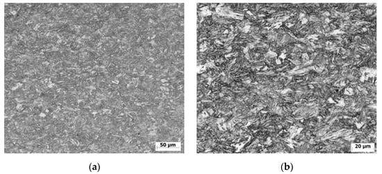
Figure 1.
Microstructure of investigated steel S960MC: (a) magnification 200×; (b) magnification 500×.
2.2. Experimental Welding
The test sample was welded to set the parameters of the physical simulation. Real courses of the temperature cycle were obtained from welding. The joint was designed as a butt weld with a square groove and root gap of 1.5 mm on 3-mm thick plates. Welding was done by means of the linear automatic machine FVD 15 MF (Fronius, Wels, Austria) with a Fronius TransPuls Synergic 2700 power source. The welding parameters were monitored with Fronius Explorer software at a frequency of 10 Hz. The following actual welding parameters were obtained by means of monitoring: mean current Iz = 102 A, wire feed speed vd = 3.8 m·s−1, mean voltage Uz = 16.6 V, and welding speed vz = 3.7 mm·s−1. Using the energy efficiency factor for MAG welding h = 0.8, the effective heat input was Qef = 0.37 kJ·mm−1.
The copper-coated solid wire Union X 96 (classified as G 89 5 M21 Mn4Ni2.5CrMo, according to the EN ISO 16834-A standard; manufactured by Böhler Welding) was used for welding. This wire belongs to undermatching filler materials, where the yield strength of the weld metal is less than the yield strength of the base material. The manufacturer’s minimum guaranteed yield strength value is Rp0.2 = 930 MPa, and the tensile strength is Rm = 980 MPa for M21 shielding gas. Filler material with the same classification for welding steels of the strength grade 960 MPa was also used in studies by Guo et al. [11], Jambor et al. [25,26], Schneider et al. [20], and Taavitsainen et al. [5]. Type MIX 18 (classification M21, manufactured by Linde) was used as the shielding gas at a gas flow of 15 L/min when welded without preheating.
During the welding process, temperature cycles in the HAZ were recorded by the Temperature Input Module NI-9212 (manufactured by National Instruments) with an application prepared in the LabView software environment. For each channel, the temperature scan rate was 95 Hz. T-type thermocouples with a diameter of 0.32 mm were condenser-welded on the bottom of the plate.
Figure 2 shows a view of the bottom of the sheet in the area of the weld root and welded thermocouples. The distance of the TC1 thermocouple from the root edge was 0.96 mm. The distance between the TC1 and TC2 thermocouples was 3.18 mm, and 4.69 mm between TC3 and TC2. The thermal effect from welding the thermocouples on the material created local craters.
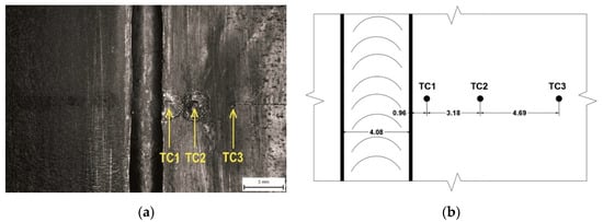
Figure 2.
Position of thermocouples on the root side of the weld: (a) marking the locations of the welded thermocouples; (b) geometry of the thermocouple position from the edge of the weld root.
Geometrical evaluation of the butt weld joint in the cross-section through an area of welded thermocouples is shown in Figure 3. The weld reinforcement was 1.71 mm at the weld width of 6.79 mm. The root reinforcement was 1.43 mm at the root weld width of 4.08 mm. The weld showed a little linear misalignment between plates.
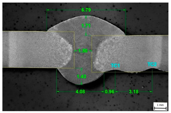
Figure 3.
Geometrical evaluation of the experimental butt weld joint with marked points of thermal cycle measurement. (unit: mm)
The thermal cycles obtained from the welding are shown in Figure 4. To determine the cooling time t8/5, the cycle temperature must be higher than 800 °C. Only the TC1 thermocouple reached a temperature above 800 °C, and its maximum temperature was 1105 °C. The cooling time t8/5 = 17.5 s was determined from the thermal cycle of the TC1 thermocouple. The maximum temperature of the TC2 thermocouple was 688 °C. This temperature indicated that the TC2 thermocouple was on the border of the HAZ and the base material. The maximum temperature of the TC3 thermocouple was 283 °C. At this temperature, there was no change in the material properties, so the thermocouple was positioned in the base material.
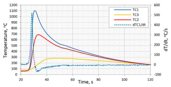
Figure 4.
Thermal cycle obtained during the welding of a S960MC steel butt weld joint.
2.3. Preparation of Input Data for Physical Simulation
Physical simulation provides a unique opportunity to describe a HAZ in steels and other metal materials for various fusion welding methods. It includes processes with a high energy density such as electron beam welding (EBW) and laser beam welding (LBW) as well as processes with a medium to low energy density such as arc welding. In this paper, HAZ physical simulations were carried out on a Gleeble 3500 thermo-mechanical physical simulator (manufactured by Dynamic Systems Inc., Poestenkill, NY, USA), which is installed at the Technical University of Liberec, Liberec, Czech Republic.
The heating and cooling of the test samples in this test was controlled according to the specified temperature cycle set to the Gleeble system—the so-called “TCprog Program Cycle”. The above-mentioned cycle can be generated based on the calculation model in QuikSIM2 software, according to the welding input conditions such as the type of material, heat input, metal sheet thickness, etc. Six functions can be used [27]. The first function is based on a real measured cycle. We can also use four equations derived from certain heat transfer equations such as the Hannerz equation, Rykalin 2D and 3D equations, and the Rosenthal equation. In the last one above-mentioned—the exponential cooling method—the sample is heated to a maximum temperature given by the rate. Then, the sample is exponentially cooled at a predetermined rate from 800 to 500 °C.
In the experiment, the method based on the description of the TCprog control cycle was used according to the measured data from the actual TC1 temperature cycle depicted in Figure 4, which was termed as the “TCref Reference Cycle” for further description. The TCref cycle consists of a heating phase, where the heating rate can be calculated as its first derivative, dT/dt. The maximum heating rate value was 522.5 °C/s and was used to determine the TCprog control cycle heating rate. The maximum heating cycle rate value was Tmax = 1105 °C. The cooling phase was described by the cooling time t8/5. The Strenx 960MC steel manufacturer recommends a t8/5 time interval of 1–15 s to ensure satisfactory mechanical properties of the weld joint [28]. For the experiment using the Gleeble instrument, three program cycles were designed with different levels of the t8/5 cooling time. These program cycles were designated as TC1prog, TC2prog, and TC3prog. The cooling time t8/5 was programmed at the following three levels: t8/5 = 7 s (for TC1prog), t8/5 = 10 s (for TC2prog), and t8/5 = 17 s (for TC3prog). At the same time and for the given test conditions, the time t8/5 = 7 s was the shortest that could be achieved using Gleeble. This was done when the control system turned off the power supply as the maximum cycle temperature was reached, and the sample was cooled through heat transfer by water-cooled jaws that clamped the sample. In the TC1prog program cycle, this phase represented the sample temperature requirement of 20 °C. Figure 5 shows the program temperature cycles used in the experiment.
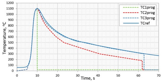
Figure 5.
Program temperature cycles for the control Gleeble.
2.4. Preparation of Test Samples and Their Physical Simulation on Gleeble
Samples are normalized when testing materials because they follow standards such as EN ISO. However, samples in a physical simulation can often be arbitrary in order to achieve a satisfactory goal of the simulation. For HAZ simulation, round bars are most often recommended for tensile tests. Samples of a square cross-section are recommended for Charpy impact tests. A higher cooling rate can be achieved in the case of round samples and shortening the free length of the sample also speeds up cooling.
Since a material of thickness t = 3 mm was used in the experiment, the samples for simulation were flat and their dimensions were modified to fit the clamping jaws. As the samples could not be clamped at their original thickness, they were reduced by grinding on both sides to a thickness of 2 mm after laser cutting. The sampling was carried out in the direction of the metal sheet rolling. The overall dimensions of the test sample for the Gleeble simulation are shown in Figure 6.
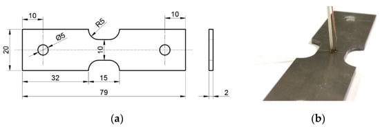
Figure 6.
Samples for testing on a Gleeble 3500 device and a tensile test after simulation: (a) dimensions of the test sample (unit: mm); (b) view of the test sample with a thermocouple welded on it.
A thermocouple was welded onto the sample—in the middle of its length—using a condenser welding machine. This thermocouple sensed the real temperature during heating and cooling. At the same time, this cycle was compared with the program cycle, and the control system adjusted the power to achieve matching of the two cycles. The sample clamping during thermal loading in the Gleeble device is shown in Figure 7.
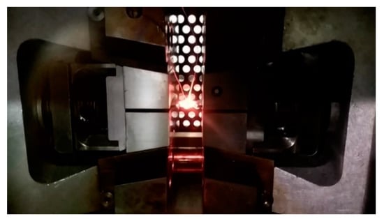
Figure 7.
Position of the sample in the Gleeble 3500 device during the temperature cycle application.
For three control cycles, three sets of test samples were prepared for the Gleeble for subsequent mechanical testing and microstructure assessment. The test samples were labeled according to their cooling time t8/5, namely 7s, 10s, and 17s. The device was set to “Force-Control” when the force F = 0. This means that the distance between the jaws changed automatically with respect to the thermal expansion of the samples. As a result, no internal stresses occurred in the samples. The whole process took place in a vacuum. A record of the real temperature cycles measured during the simulation for different times t8/5 is shown in Figure 8. In a temperature cycle corresponding to the cooling time t8/5 = 7 s, an increase in temperature can be observed at 480 °C. This increase is associated with the latent heat release during austenite transformation. A similar phenomenon can be observed in the cycle for t8/5 = 10 s. In this case, the austenite phase transformation beginning temperature shifted to 500 °C as the austenite decay temperature curve in the CCT diagram increased with time. This phenomenon was not observed in the last temperature cycle with a t8/5 = 17 s cooling time. This is because the Gleeble device was able to transfer the latent heat generated in the sample by cooling according to the program cycle already at slower cooling.
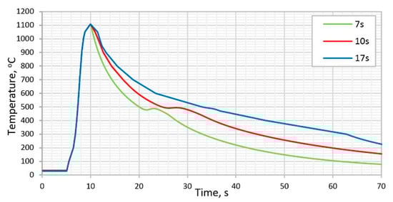
Figure 8.
Thermal cycle from the Gleeble physical simulation with different cooling times t8/5.
Samples directly from the Gleeble device were used for the static tensile test, without further treatment or modification. The test was performed on an INSTRON Model 5985 at room temperature. Figure 9 shows the samples after physical simulation milled to the required dimensions for the Charpy pendulum impact test, with a maximum impact energy of 150 J. At the same time, shims were adhered to the sample in the same way as recommended by the EN ISO 148-1 standard for low energies. The fracture surfaces after the impact test were shot by a scanning electron microscope (SEM), model TESLA VEGA II. Samples for the assessment of the microstructure and microhardness were taken by the means of a longitudinal section using precise water-cooled cutting equipment to prevent heat affecting the samples. Sample dimensions are shown in Figure 10. Samples were prepared by a standard procedure for light metallographic microscopy and etched with 2% Nital. Samples were assessed using a ZEISS LSM 700 optical microscope (Carl Zeiss Microscopy GmbH, Jena, Germany). Microhardness was measured in a line drawn through the thickness center using an Innovatest NOVA 130 device (INNOVATEST Europe BV, Maastricht, The Netherlands). This measurement utilized a load force of 9.807 N for 10 s. The distance between indentations was 0.5 mm.
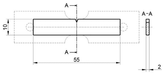
Figure 9.
Sample with a reduced thickness of 2 mm used to measure the Charpy pendulum impact test (unit: mm).
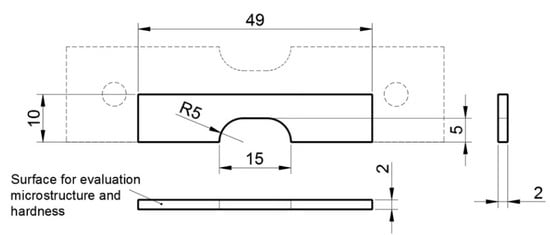
Figure 10.
Sample with a reduced thickness of 2 mm used for the microstructure and hardness evaluation (unit: mm).
3. Results and Discussion
3.1. Tensile Test and Charpy Pendulum Test
In the static tensile test, we assessed the yield strength and tensile strength. Subsequently, we used these values to calculate their mutual ratio. The Charpy pendulum impact test was carried out at the temperature of −40 °C. The sample width was 2 mm, which is not a normalized dimension. Samples of the same width were also made for the base material (BM). The average value was calculated from five measurements. The criterion value of absorbed energy for S960MC steel at −40 °C is KV = 27 J in the case of samples with a standard 10 mm width. To compare the results of 2 mm wide samples with the criterion value, the results were recalculated using a coefficient given by the ratio of reduced width and standard width (i.e., 10 mm/2 mm = 5.) The same approach was also used by Schneider et al. [20] and Guo [11] in their works.
The results of tensile testing showed that the load on the base material by a thermal cycle with a maximum temperature of 1105 °C causes a decrease in the tensile and yield strength. The cooling rate expressed by time t8/5 had a decisive influence on the above-mentioned phenomenon. The tensile test samples marked “7s” reached an average tensile strength of 1027.2 MPa, which is 94% of the value of the base material. This value is above the minimum required value of 980 MPa for the S960MC steel. The yield strength was 917.4 MPa, which is 91% of the base material value. However, it was below the minimum required yield strength of 960 MPa for the S960MC steel. In the case of the 10s and 17s samples, the tensile strength and yield strength did not reach the minimum required values for the steel that was investigated. The ratio of yield strength to tensile strength rose with an increasing cooling time t8/5 value from 0.89 in the case of the 7s sample up to 0.91 in the 17s sample. The above ratio for the base material reached 0.92. The results of the tensile test are presented in Table 3, and are graphically shown in Figure 11.
Table 3.
Results of the tensile test (at a room temperature of 23 ± 2 °C) for the base material and samples affected by the thermal cycle under different cooling times t8/5.
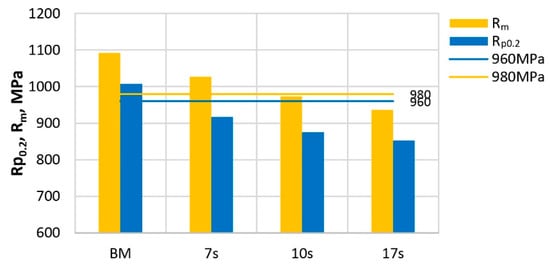
Figure 11.
Yield strength and tensile strength for the base material and samples with different cooling times t8/5.
As a result of the above-mentioned testing, the tensile strength and yield strength decrease as the t8/5 time value increases. This is a phenomenon described by other authors in their work [10,19,20]. However, even the minimum cooling time of t8/5 = 7 s that could be simulated on the Gleeble device did not achieve the required mechanical properties.
The afore-mentioned reduction in tensile strength can be explained by several aspects. In the investigated HAZ region, grain coarsening, and a higher degree of martensite tempering (lowering the degree of tetragonality) occurred, resulting in a decreased hardness and hence tensile strength. At the same time, we expect the precipitate dissolution of micro-alloying elements that lose their ability to prevent the growth of austenite grains.
In the Charpy pendulum impact tests of the assessed samples with a reduced width of 2 mm, the absorbed energy values in all simulated samples were higher than those of the base material. The test was carried out at −40 °C. This value was 20 J in the 7s sample. These values were higher in the 10s and 17s samples. The base material reached an average absorbed energy value of 17 J. At the same time, there was a trend of an increasing absorbed energy value with an increasing t8/5 cooling time. This increase can be explained by a more pronounced effect of tempering the martensitic structure in repeated heating. On the contrary, the influence of grain growth had a negative effect on the absorbed energy. The results of the Charpy pendulum impact tests are shown in Table 4 and are graphically shown in Figure 12. At the same time, this table also shows the recalculated absorbed energy values based on the dimensions of a standard 10-mm wide sample. These values in all samples were higher than the minimum required value of 27 J for the S960MC steel at −40 °C.
Table 4.
Results of the Charpy pendulum impact test (at the temperature of −40 °C) for the base material and samples affected by the thermal cycle under different cooling times t8/5.
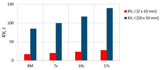
Figure 12.
Absorbed energy KV for the base material and samples with different cooling times t8/5.
3.2. Charpy Fracture Surfaces
The observation of the fracture surface topography of the broken samples after the Charpy impact tests using scanning electron microscopy (SEM) only revealed the ductile fracture. In Figure 13, it can be seen that the ductile fracture is accompanied by plastic deformation, which is manifested macroscopically by the cross-section distortion of all broken samples. Microscopically, pure transcrystalline ductile fractures with a typical dimple morphology, without any signatures of intercrystalline or brittle fracture, can be observed. The variation of dimple size is affected by the microstructural features of the HAZ. As can be seen in Figure 14, the different cooling times have a negligible influence on the fracture changes in this case. The ductile dimples are generated around carbide particles (Fe3C). Therefore, the size, shape, and distribution of dimples depend on the distribution of carbide particles and grain size.
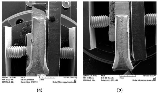
Figure 13.
SEM images of the whole fracture surface after the Charpy pendulum impact test with different cooling times t8/5: (a) sample 7s; (b) sample 17s.
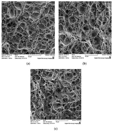
Figure 14.
SEM micrographs of the fracture surface after the Charpy pendulum impact test with different cooling times: (a) sample 7s; (b) sample 10s; (c) sample 17s.
3.3. Microstructure Analysis
The main emphasis in evaluating the microstructure was placed on comparing the structural changes in the central part of the simulated samples that were exposed to the same maximum temperature of 1105 °C, but cooled at different rates, expressed by time t8/5. Heating the base material to 1105 °C represents the transformation of the original structure into austenite, which grew at the same time. After rapid cooling, the enlarged austenitic grains were converted back to coarse martensite. This region (Figure 15a–c and Figure 16—area f) is called the coarse grain heat-affected zone (CGHAZ). Moravec et al. [22] used the temperature of 1350 °C to evaluate this zone. It is obvious that even at 1105 °C—which is highly in the austenitic region—this results in the growth of austenitic grains, a phenomenon that strongly depends on temperature and time. This growth will increase as the increasing temperature approaches the solidus temperature. Figure 15a–c show the microstructure in the center of the samples heated to the temperature of 1105 °C and cooled at different rates. The microstructure had a similar character in light microscopy evaluation. The grain size was also determined using the linear method according to EN ISO 2624, with an average grain diameter of 18 µm for the 7s sample, 17 µm for the 10s sample, and 14 µm for the 17s sample. The results show that the cooling rate had no significant effect on the grain size. A similar statement was also presented by Laitila et al. [3] in their work.
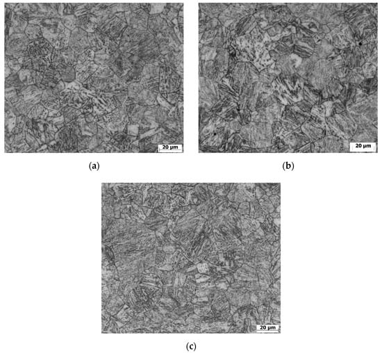
Figure 15.
Microstructure in the center of the sample with different cooling times: (a) t8/5 = 7 s; (b) t8/5 = 10 s; (c) t8/5 = 17 s.
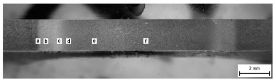
Figure 16.
Macrostructure of the 7s sample with marked spots of microstructure evaluation: (a) Base material (BM)—inter-critical heat-affected zone (ICHAZ) transition area; (b) ICHAZ area; (c) ICHAZ—fine-grained area of the heat-affected zone (FGHAZ) transition area; (d) FGHAZ area; (e) FGHAZ—coarse grain heat-affected zone (CGHAZ) transition area; (f) CGHAZ area.
In the HAZ prepared by our physical simulation, except for the coarse-grained microstructure located in the central part of the specimen, additional HAZ areas with different microstructures were visible. Similar observations in real welded joints have also been reported in works published by Jambor et al. [25,26], Guo [11], Ferreira [29], and Bayock [4]. Next to the central coarse-grained area of the HAZ, a fine-grained area of the heat-affected zone (FGHAZ) occurs. Material in the FGHAZ was heated slightly above the Ac3 temperature, but only for a very short time. This caused the transformation of the base martensitic microstructure to austenite. However, due to the relatively low temperature and a very short time of rapid cooling, which resulted in a refinement of the austenitic microstructure and, later, also of the resulting martensitic microstructure (Figure 16, area d). The last observed area of the HAZ with a changed microstructure is the region exposed to temperatures ranging from Ac1 to Ac3, where martensite was partially transformed into austenite. This temperature exposure resulted in the formation of a mixture of martensite and austenite, which, due to the slower cooling, transformed martensite into ferrite, while the untransformed martensite was tempered. The above-mentioned region is called the inter-critical heat-affected zone (ICHAZ) (Figure 16, area b). As stated in the continuous cooling transformation (CCT) diagram of S960QL steel [15,16], ferritic transformation can occur after 50–90 s in the 500–700 °C temperature range. In fact, there is a small difference in the chemical composition between S960QL and S960MC steel. The S960QL steel has a higher content of Cr and Ni, and the cooling time to the beginning of ferritic transformation will be shorter in the case of S960MC steel. Of course, some transition areas of the HAZ are also present (Figure 16a,c,e). Detailed microstructures of typical subzones of the HAZ that are formed in the S960MC steel due to different maximum temperatures of the thermal cycle and cooling rates can be seen in Figure 17.
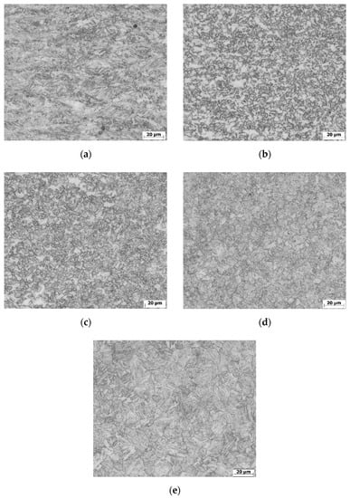
Figure 17.
Microstructure of individual subzones from the center of the 7s sample to its edge: (a) BM—ICHAZ transition area; (b) ICHAZ; (c) ICHAZ—FGHAZ transition area; (d) FGHAZ; (e) FGHAZ—CGHAZ transition area.
3.4. Hardness Test
The HV1 hardness was measured in a line on the longitudinal section surface of a Gleeble sample according to Figure 10, in the central part of the material thickness. For the evaluation of the effect of t8/5 on the resulting structure hardness, we calculated the average value using the six measurements in the range of −1.5 to 1.5 mm from the sample center. A decrease in hardness in this region compared to the base material was observed in all test samples. The base material had a hardness of 361 HV1. This value was determined as the average one obtained from five measurements. In the 7s sample, the value was lower by 33 HV1 than the base material hardness, reaching 328 HV1. In the 10s and 17s samples, the decrease was even greater at 309 HV1 and 302 HV1, respectively. The results showed that altering the thermal load of the base material to 1105 °C caused a decrease in hardness, and this is associated with a change in structure. As the cooling time t8/5 increases, a higher decrease in hardness is generated. A summary of the results is shown in Table 5, and graphically in Figure 18.
Table 5.
Result of the hardness test for the base material and the samples affected by the thermal cycle under different cooling times t8/5.
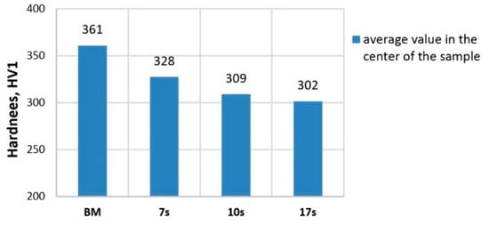
Figure 18.
Hardness values of the base material and samples with different cooling times t8/5.
4. Conclusions
Assessing the impact of welding on the change in mechanical properties, especially in HAZ high-strength steels, is a current issue and, therefore has been addressed by many researchers. The work mainly focused on steels with a thickness of 5 mm and more, where it is easier to carry out all of the required tests (especially the Charpy pendulum test). However, thin metal sheets of the S960 strength class are very often used in the manufacture of structures in order to reduce the weight. As part of our research, we performed an analysis of tensile testing, Charpy pendulum tests, fracture surfaces, and microhardness and microstructure tests in order to assess the cooling rate effect—expressed by the t8/5 time—on the change of mechanical properties of the S960MC steel HAZ. This steel was supplied at a 3 mm thickness by physical simulation using a Gleeble device. Since the Gleeble device did not allow the clamping of flat samples of such a thickness, this had to be reduced to 2 mm. The main conclusions of the above research are as follows:
- The results of the tensile test show that the loading of the base material by a temperature cycle with a maximum temperature of 1105 °C and cooling time t8/5 = 7 s caused a decrease in the tensile strength to 94% and in the yield strength to 91% of the base material values. The value of tensile strength was above the minimum required tensile strength value, but the yield strength was already below the minimum yield strength value required for S960MC steel. For the samples 10s and 17s with longer t8/5 times, this decrease was even greater and the tensile strength and yield strength did not reach the minimum values for S960MC steel. This phenomenon is associated with grain coarsening and a higher degree of martensite tempering and results in a decrease in hardness and hence strength;
- For the Charpy pendulum impact tests of samples with a reduced width of 2 mm, the absorbed energy values at the test temperature of −40 °C of all the simulated samples were higher than in the base material. At the same time, there was a trend of an increasing absorbed energy value with an increasing t8/5 cooling time. This increase can be explained—just like in strength tests—by a more pronounced effect of tempering the martensitic structure during reheating. However, the effect of grain growth in this case did not affect the absorbed energy value. After converting the absorbed energy to a standard sample width of 10 mm, all samples exceeded the KV = 27 J limit for S960MC steel. Fracture surfaces in all tested samples including the base material had the same characteristics of transcrystalline ductile fracture with a typical dimple morphology;
- Microstructure analysis was carried out in the central part of the simulated samples that were exposed to the same maximum temperature of 1105 °C, but cooled at different rates expressed by t8/5 time. The character of the microstructure was similar in all samples, consisting of coarse grains of the original austenite transformed back into martensite and tempered martensite. The grain size determined by the linear method was 18 µm for the 7s sample. A slight increase was observed for the 10s and 17s samples. The results indicate that the cooling rate had no significant effect on the grain size;
- A decrease in microhardness in the middle part of the Gleeble sample corresponding to the CGHAZ zone compared to the base material was observed in all test samples. For the 7s sample, this value was lower by 33 HV1 than the base material hardness, reaching 328 HV1. For the 10s and 17s samples, the value dropped even lower, to 309 HV1 and 302 HV1, respectively. The base material hardness was 361 HV1. The results show that thermal loading of the base material to a temperature of 1105 °C causes a decrease in hardness and is associated with a change in structure. A greater decrease in hardness is generated as the t8/5 cooling time increases;
- When MAG welding 3 mm thick S960MC steel, it is necessary to ensure that appropriate welding conditions are used so that the temperature cycle in the HAZ reaches t8/5 < 7 s. It is possible to use an external method of heat removal from the HAZ by using coolers in combination with a welding mode that generates the lowest possible heat input while maintaining weld integrity.
Author Contributions
Conceptualization, writing—original draft, and project administration, M.M.; Funding acquisition, M.M. and L.T; Data curation and formal analysis, D.H.; Investigation, D.H., F.N., and J.M; Methodology, F.N. and L.T.; Validation, J.W and J.M.; Writing—review and editing, J.W. All authors have read and agreed to the published version of the manuscript.
Funding
This research was funded by APVV, grant number APVV-16-0276; KEGA, grant number KEGA 009ŽU-4/2019; and VEGA, grant number VEGA 1/0951/17.
Conflicts of Interest
The authors declare no conflicts of interest.
References
- Schaupp, S.; Schroepfer, D.; Kromm, A.; Kannengiesser, T. Welding residual stresses in 960 MPa grade QT and TMCP high-strength steels. J. Manuf. Process. 2017, 27, 226–232. [Google Scholar] [CrossRef]
- Branco, R.; Berto, F. Mechanical Behavior of High-Strength, Low-Alloy Steels. Metals 2018, 8, 610. [Google Scholar] [CrossRef]
- Laitila, J.; Larkiola, J. Effect of enhanced cooling on mechanical properties of a multipass welded martensitic steel. Weld. World 2019, 63, 637–646. [Google Scholar] [CrossRef]
- Njock Bayock, F.; Kah, P.; Mvola, B.; Layus, P. Effect of heat input and undermatched filler wire on the microstructure and mechanical properties of dissimilar S700MC/S960QC high-strength steels. Metals 2019, 9, 883. [Google Scholar] [CrossRef]
- Taavitsainen, J.; Santos Vilaca da Silva, P.; Porter, D.; Suikkanen, P. Weldability of Direct-Quenched Steel with a Yield Stress of 960 MPa. In Proceedings of the 10th International Conference on Trends in Welding Research and 9th International Welding Symposium of Japan Welding Society (9WS), Tokyo, Japan, 11–14 October 2017; pp. 52–55. [Google Scholar]
- Ślęzaka, S.; Śnieżeka, L. Comparative LCF study of S960QL high strength steel and S355J2 mild steel. Procedia Eng. 2015, 114, 78–85. [Google Scholar] [CrossRef]
- Lago, J.; Trško, L.; Jambor, M.; Nový, F.; Bokůvka, O.; Mičian, M.; Pastorek, F. Fatigue life improvement of the high strength steel welded joints by ultrasonic impact peening. Metals 2019, 9, 619. [Google Scholar] [CrossRef]
- Hochhauser, F.; Ernst, W.; Rauch, R.; Vallant, R.; Enzinger, N. Influence of the soft zone on the strength of welded modern hsla steels. Weld. World 2012, 56, 77–85. [Google Scholar] [CrossRef]
- Björk, T.; Toivonen, J.; Nykänen, T. Capacity of fillet welded joints made of ultra high-strength steel. Weld. World 2012, 56, 71. [Google Scholar] [CrossRef]
- Nowacki, J.; Sajek, A.; Matkowski, P. The influence of welding heat input on the microstructure of joints of S1100QL steel in one-pass welding. Arch. Civ. Mech. Eng. 2016, 16, 777–783. [Google Scholar] [CrossRef]
- Guo, W.; Crowther, D.; Francis, J.A.; Thompson, A.; Liuc, Z.; Li, L. Microstructure and mechanical properties of laser welded S960 high strength steel. Mater. Des. 2015, 85, 534–548. [Google Scholar] [CrossRef]
- Guo, W.; Li, L.; Dong, S.; Crowther, D.; Thompson, A. Comparison of microstructure and mechanical properties of ultra-narrow gap laser and gas-metal-arc welded S960 high strength steel. Opt. Lasers Eng. 2017, 91, 1–15. [Google Scholar] [CrossRef]
- Kopas, P.; Sága, M.; Jambor, M.; Nový, F.; Trško, L.; Jakubovičová, L. Comparison of the mechanical properties and microstructural evolution in the HAZ of HSLA DOMEX 700MC welded by gas metal arc welding and electron beam welding. MATEC Web Conf. 2018, 244, 01009. [Google Scholar] [CrossRef]
- Górka, J. Structure and Properties of Hybrid Laser Arc Welded T-joints (Laser Beam–MAG) in Thermo-mechanical Control Processed Steel S700MC of 10 mm thickness. Arch. Metall. Mater. 2018, 63, 1125–1131. [Google Scholar]
- Sajek, A.; Nowacki, J. Comparative evaluation of various experimental and numerical simulation methods for determination of t8/5 cooling times in HPAW process weldments. Arch. Civ. Mech. Eng. 2018, 18, 583–591. [Google Scholar] [CrossRef]
- Samardžić, I.; Dunđer, M.; Katinić, M.; Krnić, N. Weldability investigation on real welded plates of fine-grained high-strength steel S960QL. Metalurgija 2017, 56, 207–210. [Google Scholar]
- Lahtinen, T.; Vilaça, P.; Peura, P.; Mehtonen, S. MAG welding tests of modern high strength steels with minimum yield strength of 700 MPa. Appl. Sci. 2019, 9, 1031. [Google Scholar] [CrossRef]
- Sefcikova, K.; Brtnik, T.; Dolejs, J.; Keltamaki, K.; Topilla, R. Mechanical properties of heat affected zone of high strength steels. IOP Conf. Ser. Mater. Sci. Eng. 2015, 96, 012053. [Google Scholar] [CrossRef]
- Pisarski, H.G.; Dolby, R.E. The significance of softened HAZs in high strength structural steels. Weld. World 2003, 47, 32. [Google Scholar] [CrossRef]
- Schneider, C.; Ernst, W.; Schnitzer, R.; Staufer, H.; Vallant, R.; Enzinger, N. Welding of S960MC with undermatching filler material. Weld. World 2018, 62, 801. [Google Scholar] [CrossRef]
- Barsoum, Z.; Khurshid, M. Ultimate strength capacity of welded joints in high strength steels. Procedia Struct. Integrity 2017, 5, 1401–1408. [Google Scholar] [CrossRef]
- Moravec, J.; Novakova, I.; Sobotka, J.; Neumann, H. Determination of grain growth kinetics and assessment of welding effect on properties of S700MC steel in the HAZ of welded joints. Metals 2019, 9, 707. [Google Scholar] [CrossRef]
- Gáspár, M. Effect of welding heat input on simulated HAZ areas in S960QL high strength steel. Metals 2019, 9, 1226. [Google Scholar] [CrossRef]
- Dunđer, M.; Vuherer, T.; Samardžić, I. Weldability prediction of high strength steel S960QL after weld thermal cycle simulation. Metalurgija 2014, 53, 627–630. [Google Scholar]
- Jambor, M.; Ulewicz, R.; Nový, F.; Bokůvka, O.; Trško, L.; Mičian, M.; Harmaniak, D. Evolution of microstructure in the heat affected zone of S960MC GMAW weld. Mater. Res. Proc. 2018, 5, 78–83. [Google Scholar]
- Jambor, M.; Novy, F.; Mician, M.; Trsko, L.; Bokuvka, O.; Pastorek, F.; Harmaniak, D. Gas metal arc welding of thermo-mechanically controlled processed S960MC steel thin sheets with different welding parameters. Commun. Sci. Lett. Univ. Zilina 2018, 20, 29–35. [Google Scholar]
- Gleeble User Training 2012. Gleeble Systems and Applications; Dynamic Systems Inc.: Poestenkill, NY, USA, 2013. [Google Scholar]
- Strenx. Welding of Strenx; SSAB AB: Stockholm, Sweden, 2017. [Google Scholar]
- Ferreira, D.N.B.; Alves, A.N.S.; Neto, R.M.A.C.; Martins, T.F.; Brandi, S.D. A New Approach to simulate HSLA steel multipass welding through distributed point heat sources model. Metals 2018, 8, 951. [Google Scholar] [CrossRef]


© 2020 by the authors. Licensee MDPI, Basel, Switzerland. This article is an open access article distributed under the terms and conditions of the Creative Commons Attribution (CC BY) license (http://creativecommons.org/licenses/by/4.0/).