Article

Reynolds Equation for a Micro-Scale Lubrication of a Gas Between Eccentric Circular Cylinders with an Arbitrary Temperature Difference Based on Slip-Flow Theory

Department of Applied Mathematics and Physics, Faculty of Engineering, Tottori University, Tottori 680-8552, Japan
Lubricants 2025, 13(8), 353; https://doi.org/10.3390/lubricants13080353 (registering DOI)
Submission received: 27 June 2025 / Revised: 29 July 2025 / Accepted: 5 August 2025 / Published: 7 August 2025
(This article belongs to the Special Issue Gas Lubrication and Dry Gas Seal, 2nd Edition)

Abstract

Micro-scale lubrication flow of a gas between eccentric circular cylinders with an arbitrary temperature difference is studied on the basis of the Navier–Stokes set of equations and the velocity slip and temperature jump boundary conditions. The dimensionless curvature, which is defined as the mean clearance divided by the radius of the inner cylinder, is small, the Knudsen number and the Reynolds number based on the mean clearance are small, and the temperature ratio is arbitrary. The Reynolds-type lubrication equation is derived analytically. For a verification of the equation, an assessment is conducted against the solution of the direct numerical analysis of the Bhatnagar–Gross–Krook–Welander (BGKW) model of the Boltzmann equation in the author’s previous work [Doi, T. Phys. Fluids 2024, 36, 042016]. The solution of the lubrication equation agrees with that of the Boltzmann equation satisfactorily well over the slip flow regime, not only in the eccentric force and the torque but also in the local distribution of the temperature, flow velocity, and the normal stress. A superiority of the lubrication equation over the lubrication model proposed in the author’s previous work is also discussed.

1. Introduction

Lubrication is indispensable in all systems involving bodies in a relative motion. The basic equation of fluid film lubrication known as the Reynolds equation has been derived from the Navier–Stokes set of equations [1,2]. When the clearance is so small that the mean free path of the gas is no longer negligible, i.e., the case referred to as micro-scale lubrication, noncontinuum effect arises. In this regime, the slip-type boundary conditions should replace the non-slip conditions [3,4,5,6]. When the clearance is much smaller and comparable with the mean free path, however, an analysis on the basis of kinetic theory is necessary [7,8,9,10,11,12]. For a lubrication between nearly parallel planes, a generalized lubrication equation valid for an arbitrary Knudsen number has been derived [8], where the Knudsen number is defined as the mean free path divided by the reference clearance. A more systematic derivation including curved geometries is given in [12].
Some attempts to extend the analysis in [12] to a system between walls with a large temperature difference have been made [13], motivated by the heat-assisted magnetic recording in a hard disk drive [14]. In [13], a micro-scale lubrication flow between nearly parallel planes with an arbitrary temperature difference was studied on the basis of the Boltzmann equation. A serious problem is that the method of analysis in [12] is inapplicable when the leading order solution of the perturbation is a nonequilibrium state, and this is the case when a large temperature difference is present. In [13], a crude approximation is employed that the leading order solution is replaced by the free molecular solution. Using this approximation and the Bhatnagar–Gross–Krook–Welander (BGKW) kinetic model [15,16] as the basic equation, a Reynolds-type macroscopic lubrication equation has been derived in a closed form. An assessment of this equation against the direct numerical analysis of the BGKW model of the Boltzmann equation has confirmed that this lubrication model produces a satisfactory solution not only for a large Knudsen number but also even for a small Knudsen number down to 0.1.
In our previous paper [17], we applied this approximation method to a lubrication system between rotating eccentric circular cylinders with a large temperature difference, and derived a macroscopic lubrication model. The result of an assessment showed that this lubrication equation yields a good approximation to that of the Boltzmann equation for a large Knudsen number, but the approximation fails for a small Knudsen number. Therefore, we were forced to devise another lubrication equation that covers a region of small Knudsen numbers. A candidate was that the leading order solution is replaced by a Maxwellian distribution the temperature of which is the solution of the heat conduction equation. The lubrication equation derived in this way (say, model B in [17]) actually provides a good approximation to the solution of the Boltzmann equation for a small Knudsen number, but the approximation becomes rapidly worse as the Knudsen number increases. To be specific, model B is applicable only for a small Knudsen number up to 0.1. However, one may wonder if we are aiming to introduce a lubrication model that works only for a regime of small Knudsen numbers, then we may rely on the slip flow theory [10]. This is favorable for the following reasons. The model B contains some functions, given in the database, which are obtained by numerically solving the spatially one-dimensional (1D) Boltzmann equation. These functions depend on the parameters of configuration, e.g., eccentricity of the system. Thus, if one wishes to use the model for other parameters that were not given in [17], then additional numerical analysis of the Boltzmann equation is necessary to furnish the model. Therefore, considerable knowledge on kinetic theory and numerical techniques are required. In contrast, the analysis based on the slip flow theory will be accessible to a wide variety of scientists and engineers. In addition, the lubrication equation will be derived analytically by the latter approach.
In the present paper, we study a micro-scale lubrication flow of a gas between eccentric circular cylinders with an arbitrary temperature difference on the basis of the Navier–Stokes set of equations and the velocity slip and temperature jump boundary conditions. The dimensionless curvature, which is defined as the mean clearance divided by the radius of the inner cylinder, is small, the Knudsen number and the Reynolds number based on the mean clearance are small, and the temperature ratio is arbitrary. The Reynolds-type lubrication equation is derived analytically. For a verification of this equation, an assessment against the solution of the direct numerical analysis of the BGKW model of the Boltzmann equation in [17] is conducted. The goals of this paper are as follows: (i) we present the lubrication equation analytically, (ii) we verify that the solution of this lubrication equation approximates that of the Boltzmann equation at least in the slip flow regime, and (iii) we also compare it with the result of model B in [17], and discuss the performance and actual usability over it. Incidentally, Milićev and Stevanović actively study the effect of temperature difference on micro-scale lubrication [18,19]. The present study is similar to [19]. Main differences in the present work from [19] are as follows: first, the former concerns an eccentric annulus whereas the latter concerns nearly parallel planes, second, the former does not take the effect of the convection term into account, and third, the former derives the Reynolds equation in a more familiar form not expanded in the Knudsen number.

2. Problem and Basic Equations

2.1. Problem

Let us consider a monatomic ideal gas in the annulus between eccentric circular cylinders as shown in Figure 1a, where X i is the Cartesian coordinate system. The radius of the inner cylinder is r a , that of the outer cylinder is r b , and the distance between the two axes is e c . The inner and outer cylinders rotate at constant circumferential velocities v w a and v w b , respectively. The v w a and v w b are positive when the rotation is counterclockwise. For the reference speed, we denote max ( | v w a | , | v w b | ) by v w . The temperature of the inner cylinder is a constant T a , and that of the outer cylinder is a constant T b . We denote min ( T a , T b ) by T 0 , and refer to “inner heating” when T a > T b , and “outer heating” when T a < T b for brevity. The dimensionless curvature c is defined as c = ( r b r a ) / r a . The rarefaction parameter k is defined by k = ( π / 2 ) 0 / ( r b r a ) , where 0 is the mean free path of the gas in the equilibrium state at rest with the average density ρ 0 of the gas and the temperature T 0 ; we call k as the Knudsen number for simplicity. Note that the inverse Knudsen number 1 / k is often used as the rarefaction parameter in the literature on lubrication, but we use k in accordance with [17]. Let c be small, and let the reference speed v w also be small compared with the sonic speed. The eccentricity ε = e c / ( r b r a ) is arbitrary, but it is not close to unity. To be specific,
c k 1 , v ^ w = O ( c ) , 1 ε = O ( 1 ) ,
where v ^ w = v w / ( 2 R T 0 ) 1 / 2 is a quantity of the order of the Mach number; R is the specific gas constant, i.e., the Boltzmann constant divided by the mass of a molecule. According to kinetic theory [12], the viscosity μ and the heat conductivity λ of a monatomic ideal gas is a function of the gas temperature. In this paper, we assume that μ and λ are proportional to the n-th power of the gas temperature T:
μ = μ 0 T T 0 n , λ = λ 0 T T 0 n ( n 0 ) ;
the values μ 0 and λ 0 at the temperature T 0 are related to the mean free path 0 by [12]
μ 0 = π 2 γ 1 p 0 ( 2 R T 0 ) 1 / 2 0 , λ 0 = 5 π 4 γ 2 R p 0 ( 2 R T 0 ) 1 / 2 0 ,
where p 0 = R ρ 0 T 0 , and γ 1 and γ 2 are numbers determined by the molecular model. Therefore, the Reynolds number Re satisfies
c Re 1 where Re = ρ 0 v w ( r b r a ) μ 0 = 2 v ^ w γ 1 k .
We also denote
v w a ( 2 R T 0 ) 1 / 2 = v ^ w a = c u w a , v w b ( 2 R T 0 ) 1 / 2 = v ^ w b = c u w b ,
where u w a and u w b are constants of O ( 1 ) . We study the time-independent and axially uniform behavior of the gas on the basis of the Navier–Stokes set of equations and the velocity slip and temperature jump boundary conditions in the slip flow regime (1). The same problem has been studied on the basis of the BGKW model of the Boltzmann equation over the entire range of the Knudsen number k in [17].

2.2. Basic Equation

Let us introduce the dimensionless variables
x = X r b r a , u = v v w , p ^ = p p 0 , T ^ = T T 0 , ρ ^ = ρ ρ 0
for the spatial coordinates X , the flow velocity v , the pressure p, the temperature T, and the density ρ .
In the following analysis, we use the bipolar coordinate system ( η , χ ) , as shown in Figure 1b, defined by
x 1 = α sinh η cosh η cos χ , x 2 = α sin χ cosh η cos χ ,
u = u χ e η + u η e χ ,
where
α = ( c ε ) 1 ( 1 ε 2 ) 1 + c + 1 ε 2 4 c 2 1 / 2 .
The independent variables η and χ lie in η a η η b and 0 χ < 2 π , where η a and η b are negative constants
η a = arcsinh c α , η b = arcsinh c α 1 + c , η a < η b < 0 .
In Equation (8), e η and e χ are unit vectors in the x 1 x 2 plane normal to the curves η = const and χ = const , respectively. The scale factor h = [ ( x 1 / η ) 2 + ( x 2 / η ) 2 ] 1 / 2 = [ ( x 1 / χ ) 2 + ( x 2 / χ ) 2 ] 1 / 2 is given by
h = α cosh η cos χ .
The dimensionless Navier–Stokes set of equations in the bipolar coordinate system are given by
( h ρ ^ u η ) η + ( h ρ ^ u χ ) χ = 0 ,
ρ ^ u η h u η η + u χ h u η χ + sinh η α u χ 2 sin χ α u η u χ = 1 2 v ^ w 2 h p ^ η + T ^ n Re 1 h χ 1 h 2 h u χ η 1 h 2 h u η χ + 4 3 h div u η + n T ^ n 1 Re 2 1 h u η η sin χ α u χ 1 3 div u 1 h T ^ η + 1 h u χ η + 1 h u η χ + sin χ α u η + sinh η α u χ 1 h T ^ χ ,
ρ ^ u η h u χ η + u χ h u χ χ + sin χ α u η 2 sinh η α u χ u η = 1 2 v ^ w 2 h p ^ χ + T ^ n Re 1 h η 1 h 2 h u χ η 1 h 2 h u η χ + 4 3 h div u χ + n T ^ n 1 Re 2 1 h u χ χ sinh η α u η 1 3 div u 1 h T ^ χ + 1 h u χ η + 1 h u η χ + sin χ α u η + sinh η α u χ 1 h T ^ η ,
ρ ^ u η h T ^ η + u χ h T ^ χ = 1 Pr Re h 2 2 Γ ( T ^ ) η 2 + 2 Γ ( T ^ ) χ 2 ,
ρ ^ = p ^ / T ^ ,
where
div u = 1 h 2 h u η η + h u χ χ .
Equations (12)–(16) correspond, respectively, to the continuity equation, equations of motion in the η and χ directions, energy equation, and the equation of state. The factor ( 2 v ^ w 2 ) 1 appears in the pressure-gradient terms in (13) and (14) because we use the dimensionless pressure p ^ = p / p 0 here rather than p / ( ρ 0 v w 2 ) . The factor T ^ n in the second terms on the right-hand sides of (13) and (14) is the dimensionless viscosity μ / μ 0 , cf. (2). The third terms on the right-hand sides of (13) and (14) multiplied by n T ^ n 1 are those arising from the temperature dependence of the viscosity. In the energy Equation (15), the dissipation term is omitted because of a small Mach number, and the right-hand side is arranged using · ( T ^ n T ^ ) = · Γ where
Γ ( T ^ ) = 1 n + 1 T ^ n + 1 .
The Pr = 5 R μ 0 / ( 2 λ 0 ) is the Prandtl number for a monatomic gas, which is equal to γ 1 / γ 2 by (3).
The velocity slip and temperature jump boundary conditions are given by
u χ + k p ^ k 0 Θ ( T ^ a ) h a u χ η = v ^ w a v ^ w , u η = 0 ( η = η a ) ,
u χ k p ^ k 0 Θ ( T ^ b ) h b u χ η = v ^ w b v ^ w , u η = 0 ( η = η b ) ,
T ^ k p ^ d 1 Θ ( T ^ a ) h a T ^ η = T ^ a ( η = η a ) ,
T ^ + k p ^ d 1 Θ ( T ^ b ) h b T ^ η = T ^ b ( η = η b ) .
Here, k 0 and d 1 are the slip and jump coefficients [12] which depend on the molecular model, e.g., k 0 = 1.016 and d 1 = 1.303 for the BGKW model and the diffuse-reflection boundary condition, and h at η = η a and η = η b are denoted by h a and h b , respectively. Θ ( T ^ ) is a function determined by the molecular model [12]; e.g., Θ ( T ^ ) = T ^ 3 / 2 for the BGKW equation. The T ^ a = T a / T 0 and T ^ b = T b / T 0 are the dimensionless temperatures of the cylinders. The unknown p ^ enters the boundary conditions (18)–(21) because the pressure variation is so large that the mean free path varies significantly. Equations (18)–(21) are taken from the asymptotic theory [12] of the Boltzmann equation for a small Knudsen number in which finite gradients both in the velocity and the temperature are present.
The average gas density ρ 0 is defined by ρ d X 1 d X 2 = π ( r b 2 r a 2 ) ρ 0 , where the spatial integration is conducted over the annular region in Figure 1a. In terms of the dimensionless quantities, this equation yields
0 2 π d χ η a η b h 2 ρ ^ d η = 2 π c 1 + c 2 .
The dimensionless counterparts p ^ η η = p η η / p 0 and p ^ χ η = p χ η / p 0 of the normal and shear components p η η and p χ η of the stress are given by
p ^ η η = p ^ 2 v ^ w 2 Re T ^ n 2 h u η η 2 sin χ α u χ 2 3 div u ,
p ^ χ η = 2 v ^ w 2 Re T ^ n 1 h u χ η + 1 h u η χ + sin χ α u η + sinh η α u χ .
The Cartesian components ( F 1 , F 2 ) of the force and the torque N acting on the inner cylinder per unit depth are given by
1 p 0 r a F 1 F 2 = 0 2 π p ^ η η cos θ p ^ χ η sin θ p ^ η η sin θ + p ^ χ η cos θ c h d χ ( η = η a ) ,
N p 0 r a 2 = 0 2 π p ^ χ η c h d χ ( η = η a ) ,
where θ is the angle shown in Figure 1b defined by
cos θ = cosh η cos χ 1 cosh η cos χ , sin θ = sinh η sin χ cosh η cos χ .
N > 0 when the torque is counterclockwise in Figure 1a.

2.3. Preparation for Analysis

For convenience of the analysis in Section 3, the following re-scaling is introduced. Because η b η a = O ( c ) 1 , let us introduce the stretched coordinate y for η , the normalized scale factor H, and the constant γ as [17]
y = ( η η a ) / ( η b η a ) , H = c h = sinh η a cosh η cos χ , γ = η b η a c .
The y lies in 0 < y < 1 , and H and γ are of O ( 1 ) . η should be understood as η = η a + ( η b η a ) y in what follows, according to (28).
In terms of the new set of independent variables y and χ , the Navier–Stokes set of equations are written as
( H ρ ^ u η ) y + c γ ( H ρ ^ u χ ) χ = 0 ,
ρ ^ u η γ H u η y + c u χ H u η χ c sinh η sinh η a u χ 2 + c sin χ sinh η a u η u χ = 1 2 v ^ w 2 γ H p ^ y + T ^ n Re 1 H χ c γ H 2 H u χ y c 2 H 2 H u η χ + 4 3 γ H div u y + n T ^ n 1 Re 2 1 γ H u η y + c sin χ sinh η a u χ 1 3 div u 1 γ H T ^ y + 1 γ H u χ y + c H u η χ c sin χ sinh η a u η c sinh η sinh η a u χ c H T ^ χ ,
ρ ^ u η γ H u χ y + c u χ H u χ χ c sin χ sinh η a u η 2 + c sinh η sinh η a u χ u η = c 2 v ^ w 2 H p ^ χ + T ^ n Re 1 γ H y 1 γ H 2 H u χ y c H 2 H u η χ + c 4 3 H div u χ + n T ^ n 1 Re 2 c H u χ χ + c sinh η sinh η a u η 1 3 div u c H T ^ χ + 1 γ H u χ y + c H u η χ c sin χ sinh η a u η c sinh η sinh η a u χ 1 γ H T ^ y ,
ρ ^ u η γ H T ^ y + c u χ H T ^ χ = 1 Pr Re H 2 1 γ 2 2 Γ ( T ^ ) y 2 + c 2 2 Γ ( T ^ ) χ 2 ,
ρ ^ = p ^ / T ^ ,
where
div u = 1 H 2 1 γ H u η y + c H u χ χ .
The slip and jump boundary conditions and the subsidiary condition (22) are written as
u χ + k p ^ k 0 Θ ( T ^ a ) γ H a u χ y = v ^ w a v ^ w , u η = 0 ( y = 0 ) ,
u χ k p ^ k 0 Θ ( T ^ b ) γ H b u χ y = v ^ w b v ^ w , u η = 0 ( y = 1 ) ,
T ^ k p ^ d 1 Θ ( T ^ a ) γ H a T ^ y = T ^ a ( y = 0 ) ,
T ^ + k p ^ d 1 Θ ( T ^ b ) γ H b T ^ y = T ^ b ( y = 1 ) ,
0 2 π d χ 0 1 H 2 p ^ T ^ d y = 2 π γ 1 + c 2 ,
where H a = c h a and H b = c h b .
The normal and shear components of the dimensionless stress are
p ^ η η = p ^ 2 v ^ w 2 Re T ^ n 2 γ H u η y + 2 c sin χ sinh η a u χ 2 3 div u ,
p ^ χ η = 2 v ^ w 2 Re T ^ n 1 γ H u χ y + c H u η χ c sin χ sinh η a u η c sinh η sinh η a u χ .
The components ( F 1 , F 2 ) of the force and the torque N are given by
1 p 0 r a F 1 F 2 = 0 2 π p ^ η η cos θ p ^ χ η sin θ p ^ η η sin θ + p ^ χ η cos θ H d χ ( y = 0 ) ,
N p 0 r a 2 = 0 2 π p ^ χ η H d χ ( y = 0 ) ,
where θ is given by (27).
The boundary value problem (29)–(38) is characterized by the following dimensionless parameters:
c = r b r a r a , ε = e c r b r a , v ^ w a = v w a ( 2 R T 0 ) 1 / 2 , v ^ w b = v w b ( 2 R T 0 ) 1 / 2 ,
T ^ a = T a T 0 , T ^ b = T b T 0 , k = π 2 0 r b r a ,
and Pr, where Re is given by (4). Under the condition (1), we study this problem. Our goal is to derive a Reynolds equation that is correct up to O ( c ) .

3. Analysis

The basic equations stated in Section 2.3 are analytically studied here. The present method is a standard one deriving the Reynolds lubrication equation, and is a straightforward extension of the isothermal case in [20].
From the boundary conditions (34) and (35), we find u χ = O ( 1 ) . Substituting this into the continuity Equation (29), we obtain
u η = c γ H ρ ^ 0 y ( H ρ ^ u χ ) χ d y = O ( c ) .
Thus, div u = O ( c ) .
Neglecting the terms of O ( c Re ) , the energy Equation (32) reduces to
2 Γ ( T ^ ) y 2 = 0 .
Thus, the solution is independent of Pr. Then, Γ ( T ^ ) is a linear function of y, and thus
T ^ = ( a y + b ) ν ,
where ν = 1 / ( n + 1 ) . The a and b, which are independent of y but dependent on χ , are determined by the temperature jump conditions (36) and (37). Substituting (46) into (36) and (37) yields the nonlinear simultaneous equations
b ν δ a ν a b ν 1 = T ^ a , ( a + b ) ν + δ b ν a ( a + b ) ν 1 = T ^ b ,
δ a = k p ^ d 1 Θ ( T ^ a ) γ H a , δ b = k p ^ d 1 Θ ( T ^ b ) γ H b .
Note that a and b are undetermined unless p ^ is known because δ a and δ b depend on p ^ .
Multiplying both sides of (30) by c, and noting that T ^ / y and T ^ / χ are of O ( 1 ) , we obtain
c Re 2 v ^ w 2 p ^ y = O ( c 2 ) .
That is, c Re ( 2 v ^ w 2 ) 1 p ^ is independent of y up to O ( c ) . On the other hand, by neglecting the terms of O ( c Re ) in (31), we obtain
y 1 H 2 H u χ y + ( 1 ν ) a γ a y + b 1 γ H u χ y c sinh η sinh η a u χ = c Re γ 2 2 v ^ w 2 ( a y + b ) 1 ν d p ^ d χ .
We can further simplify this equation by using H / y = O ( c H ) and neglecting the terms of O ( c 2 ) , to yield
2 u χ y 2 + ( 1 ν ) a a y + b u χ y c ( 1 ν ) a a y + b γ H sinh η sinh η a u χ = c γ 1 Re 2 v ^ w 2 γ 2 H γ 1 ( a y + b ) 1 ν p ^ k k p ^ d p ^ d χ .
The second and the third terms on the left-hand side of (50) arise due to the temperature dependence of the viscosity. Equation (50) and the boundary conditions (34) and (35) constitute the linear and inhomogeneous boundary value problem to determine u χ that is correct up to O ( c ) . Because of the linearity, the solution is given by
u χ = c γ 1 Re 2 v ^ w 2 k p ^ d p ^ d χ u P y ; k p ^ , χ + v ^ w a v ^ w u Ca y ; k p ^ , χ + v ^ w b v ^ w u Cb y ; k p ^ , χ = c v ^ w 1 p ^ d p ^ d χ u P y ; k p ^ , χ + v ^ w a c u Ca y ; k p ^ , χ + v ^ w b c u Cb y ; k p ^ , χ ,
where (4) is used. Here, u P ( y ; k ˜ , χ ) , u Ca ( y ; k ˜ , χ ) , and u Cb ( y ; k ˜ , χ ) are solutions of the following linear boundary value problems: for u P ( y ; k ˜ , χ ) (Poiseuille flow),
2 u P y 2 + ( 1 ν ) a a y + b u P y c ( 1 ν ) a a y + b γ H sinh η sinh η a u P = γ 2 H γ 1 k ˜ ( a y + b ) 1 ν ,
u P β a u P y = 0 ( y = 0 ) , u P + β b u P y = 0 ( y = 1 ) ,
for u Ca ( y ; k ˜ , χ ) (Couette flow for rotation of the inner cylinder),
2 u Ca y 2 + ( 1 ν ) a a y + b u Ca y c ( 1 ν ) a a y + b γ H sinh η sinh η a u Ca = 0 ,
u Ca β a u Ca y = 1 ( y = 0 ) , u Ca + β b u Ca y = 0 ( y = 1 ) ,
and for u Cb ( y ; k ˜ , χ ) (Couette flow for rotation of the outer cylinder),
2 u Cb y 2 + ( 1 ν ) a a y + b u Cb y c ( 1 ν ) a a y + b γ H sinh η sinh η a u Cb = 0 ,
u Cb β a u Cb y = 0 ( y = 0 ) , u Cb + β b u Cb y = 1 ( y = 1 ) ,
where
β a = k ˜ k 0 Θ ( T ^ a ) γ H a , β b = k ˜ k 0 Θ ( T ^ b ) γ H b ,
and k ˜ is the parameter that stands for k / p ^ . The analytical solutions u P , u Ca , and u Cb are presented in Appendix A because they are lengthy. The solution (51) is still undetermined unless p ^ ( χ ) is known.
The mass conservation law serves to determine the dimensionless pressure p ^ as follows. On evaluating (44) at y = 1 , we obtain
d d χ 0 1 γ H ρ ^ u χ d y = 0 .
Substituting (51), (33), and (46) into (59), we obtain
d d χ m P k p ^ , χ d p ^ d χ + u w a p ^ m Ca k p ^ , χ + u w b p ^ m Cb k p ^ , χ = 0 ,
where m P ( k ˜ , χ ) , m Ca ( k ˜ , χ ) , and m Cb ( k ˜ , χ ) , which may be called the flow-rate coefficients, are defined by
m J = γ 0 1 H T ^ u J d y ( J = P , Ca , or Cb ) .
Equation (60) is the Reynolds equation derived from the Navier–Stokes set of equations and the velocity slip and temperature jump boundary conditions. Equation (60) is of the same form as that derived from the Boltzmann equation in [20] except for the details of m P , m Ca , and m Cb , which are given by (A15) and (A16) in Appendix A. The process to construct the solution is to be given in the next paragraph. The flow-rate coefficients in (60) contain p ^ through the first argument k / p ^ , because the slip factors in (34) and (35) as well as the factors a and b in (47) contain or depend on k / p ^ . The components of the stress that are correct up to O ( c ) are
p ^ η η = p ^ ,
p ^ χ η = c d p ^ d χ S P y ; k p ^ , χ + u w a p ^ S Ca y ; k p ^ , χ + u w b p ^ S Cb y ; k p ^ , χ ,
where S P ( y ; k ˜ , χ ) , S Ca ( y ; k ˜ , χ ) , and S Cb ( y ; k ˜ , χ ) are given by (A17) and (A18) in Appendix A.
Based on these preparations, the solution is numerically constructed as follows. The interval 0 χ 2 π is divided into N x sections, and the mesh points are arranged. An artificial “time derivative term” is added on the left-hand side of the Reynolds Equation (60). This diffusion-type partial differential equation is discretized using the finite-difference method. An initial guess of the dimensionless pressure p ^ ( χ ) is given. Then, (i) Equation (47) is solved using the Newton method to obtain a and b at every mesh point, (ii) the flow-rate coefficients m P , m Ca , and m Cb are computed from these a and b using (A15) and (A16), and (iii) the above diffusion-type equation is solved by one “time” step subject to the subsidiary condition (38) and the periodic condition p ^ ( 0 ) = p ^ ( 2 π ) , to obtain the pressure p ^ at the new time step. (iv) Repeat (i)–(iii) until the distributions of the pressure, a, and b converge. (v) Once p ^ , a, and b have converged, the temperature, flow velocity, and the stress components are given by (46), (51), (62), and (63), respectively. Finally, the eccentric force and the torque are given by (41) and (42), respectively. The convergence is very fast; the total CPU time is less than two seconds using a consumer personal computer.
Incidentally, some features of the present computational process are mentioned compared with that in [19]. In [19], the solution was expanded in the small parameter k. Owing to this, the process of solving the nonlinear Equation (47) was unnecessary. Instead, the Reynolds Equation (60) was obtained in an expanded form there. Thus, the first order equation was first solved, and subsequently, the second order one was solved with the first order solution as the inhomogeneous term. In the present analysis, the Reynolds equation is derived in the unexpanded form (60). Therefore, an actual numerical analysis is as easy as that of the conventional Reynolds equation except for the process of solving (47).

4. Results and Discussion

4.1. Preliminary Remarks

In this section, the solution of the Reynolds Equation (60) derived in Section 3 is assessed. The reference solution for this assessment is the solution of the direct numerical analysis of the BGKW model of the Boltzmann equation presented in [17]. The latter equation is valid for an arbitrary values of the parameters (43). For the BGKW model, the viscosity μ and the heat conductivity λ are both proportional to the gas temperature [12]. So we set
n = 1 thus ν = 1 / 2 , k 0 = 1.016 , d 1 = 1.303 , γ 1 = 1 , Θ ( T ^ ) = T ^ 3 / 2 .
In the assessment below, we present the cases for
v ^ w a = 0.1 , v ^ w b = 0 , ε = 0.5 ,
and ( T ^ a , T ^ b ) = ( 2 , 1 ) for the inner heating and and ( T ^ a , T ^ b ) = ( 1 , 2 ) for the outer heating. Therefore, v ^ w = 0.1 . The profiles of the physical variables, such as the normal stress, are presented for k = 0.1 , which is usually regarded as the upper limit of the slip flow regime.
The numerical computation of the Reynolds Equation (60) is conducted for N x = 100 , and the convergence of iteration is judged when the variation in p ^ at each iteration step is less than 10 8 . For a test of numerical accuracy, we conducted additional runs, namely, N x = 50 and N x = 200 for some typical cases. Judging from the differences among the three runs, the numerical error in the eccentric force (66) of the production run N x = 100 is estimated to be less than 0.06%.
In Section 4.3, another lubrication model proposed in [17] is also presented. This model is of the same form as (60). The difference from (60) is that the coefficients m P , m Ca , and m Cb are derived from the spatially 1D Boltzmann equation, and are provided as a numerical database constructed from a numerical analysis of this equation, see Appendix B in [17]. For short, this model is referred to as model B as termed in [17].
Further details of the physical discussion are presented in [17].

4.2. Temperature, Velocity, and the Normal Stress

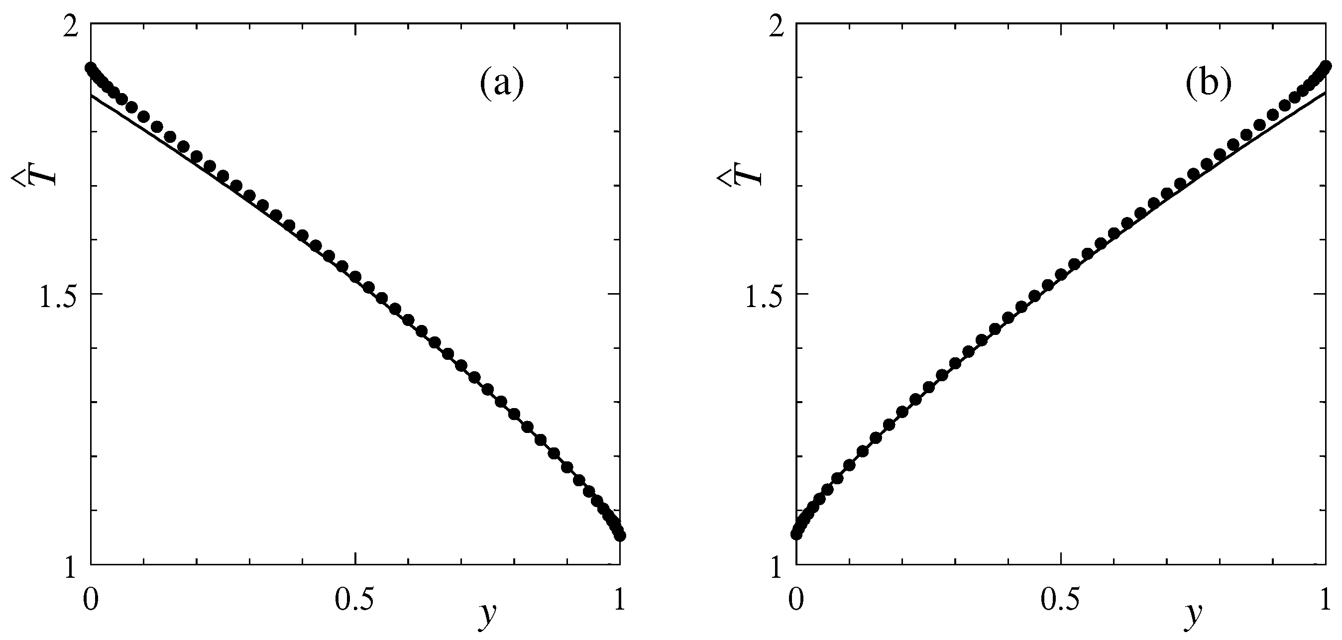
We first present the profile of the gas temperature at the cross section χ = 0 for the Knudsen number k = 0.1 in Figure 2. The solid line represents the present solution (46), and the closed circle represents the reference solution. The panel (a) is the case of inner heating, and (b) is the case of outer heating. These rules apply in the rest of this paper. The present solution agrees very well with the reference solution in the bulk of the gas. A slight disagreement is observed in a neighborhood of the heated cylinder. This disagreement is inevitable because the Knudsen layer correction [12] is not taken into account in the solution in Section 3. The temperature profile as a function of y does not depend on χ much, and the agreement at other cross sections is as good as that in Figure 2.
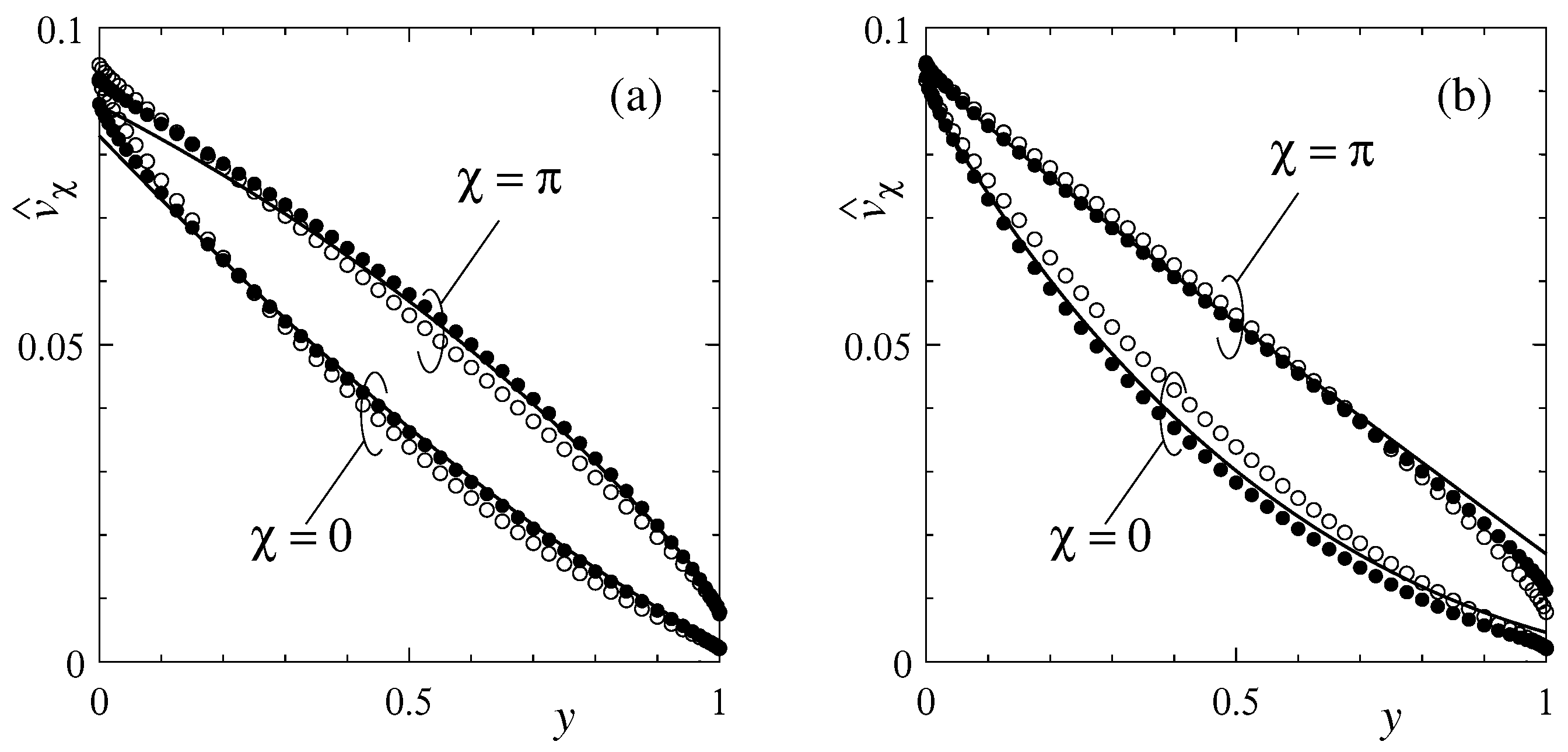
Next, the velocity profiles at the cross sections χ = 0 and π are presented in Figure 3. The open circles represent the unheated case, i.e., T a = T b . The pressure gradient is d p ^ / d χ > 0 at χ = 0 and d p ^ / d χ < 0 at χ = π . According to (51), a flow caused by the pressure gradient (Poiseuille flow) is superposed on the flow (Couette flow) induced by the rotation of the inner cylinder. As a result, the latter flow is reduced by the former flow at χ = 0 whereas enhanced at χ = π because u P in (51) is negative. The present solution agrees with the reference solution well. A slight disagreement is observed in a neighborhood of the heated cylinder, as expected from Figure 2.
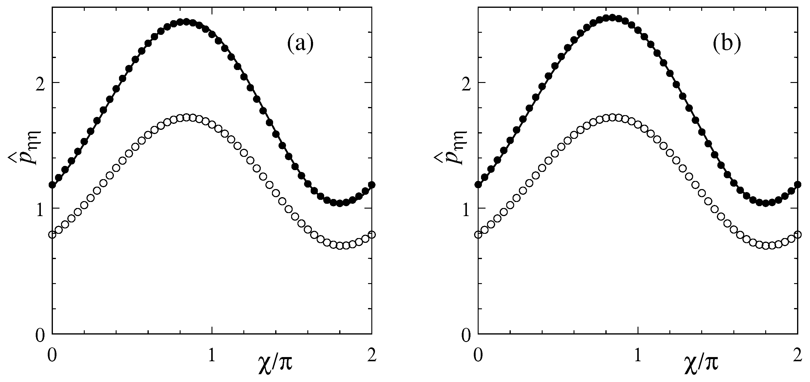
The distribution of the normal stress p ^ η η along the channel is presented in Figure 4 as a function of χ . For the reference solution, p ^ η η along the inner cylinder ( y = 0 ) is presented. We compare the normal stress p ^ η η rather than the pressure because, first, the normal force acting on the cylinder’s surface is not the pressure but the normal stress, see (41), and second, the pressure varies significantly with y due to the Knudsen layer of the temperature jump [12]. The channel is converging in 0 < χ < π as shown in Figure 1. Therefore, as the gas proceeds, the pressure and so the normal stress increases toward χ = π by the wedge action, to form the maximum around χ = π . The normal stress as well as the pressure increases due to heating either of the cylinders, because a temperature rise simply raises the pressure of a confined gas, even if the gas is at rest. When the gas is in motion, the amplitude of the pressure variation is enlarged due to the pressure rise, resulting in an enhancement of the eccentric force to appear in Section 4.3. The present solution (solid line) agrees with the reference solution (closed symbols) perfectly. Note that the agreement is good even on the heated cylinder, see Figure 4a, in contrast to Figure 2 and Figure 3. This is because the normal stress p ^ η η is not subject to the Knudsen layer correction [12] in contrast to the temperature and velocity. The p ^ y y of the reference solution is almost independent of y.

4.3. Eccentric Force and Torque

Here, we define the magnitude F and the direction ϑ F of the eccentric force (41) as
F 1 = F cos ϑ F , F 2 = F sin ϑ F .
The directions ϑ F = 0 and ϑ F = π / 2 correspond to X 1 and X 2 directions in Figure 1a, respectively.
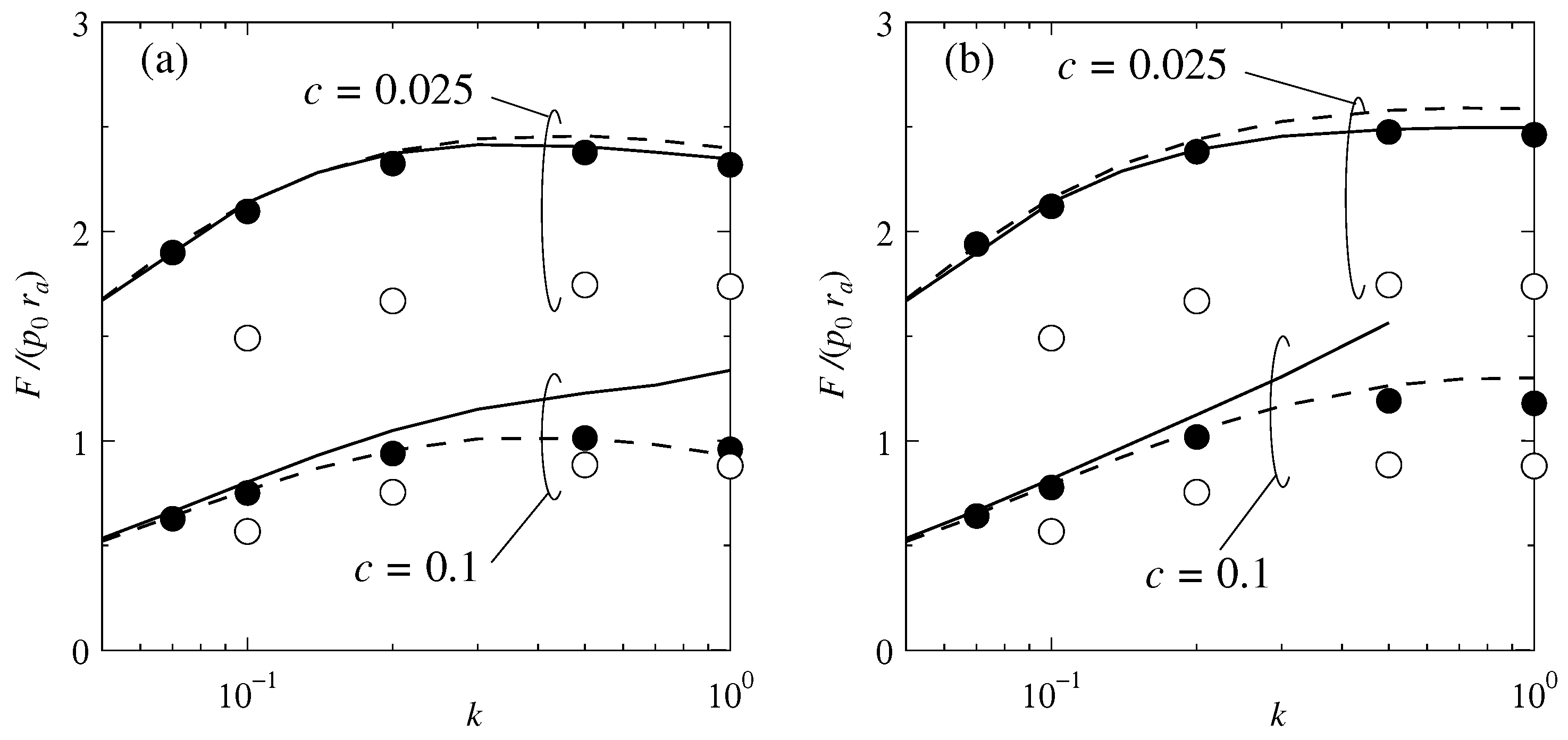
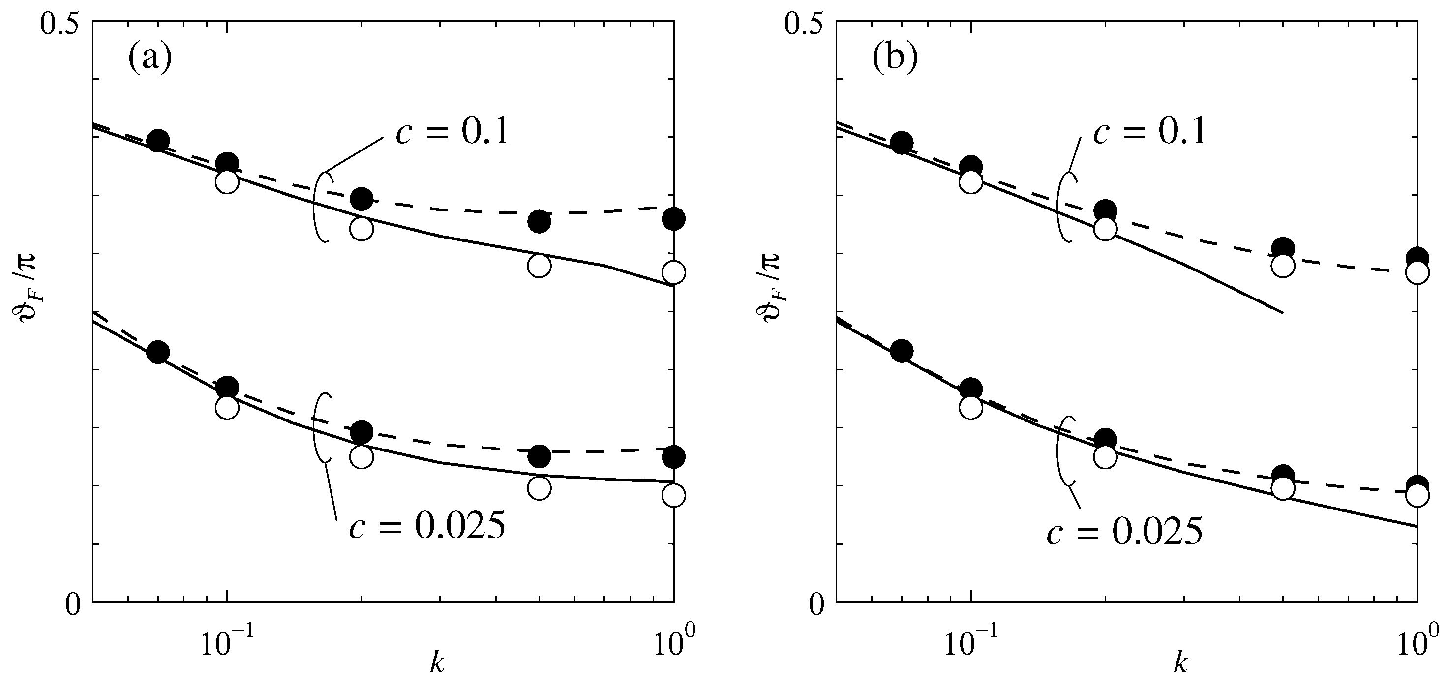
The magnitude F and the direction ϑ F are presented in Figure 5 and Figure 6, respectively, as functions of the Knudsen number k. In the figures, the result of model B is also presented in the dotted line for comparison. The open circles represent the unheated case. The eccentric force is enhanced by heating either of the cylinders, as noted in Section 4.2, but the magnitude does not depend much on which cylinder is heated. This is a characteristic of the effect of heating for a small Knudsen number [17]. Let us start the assessment. For k 0.1 , both the present solution and model B agree with the reference solution very well. Beyond k = 0.1 , non-negligible disagreement is observed in both models. The present solution is better with respect to the magnitude F in Figure 5, whereas model B is better with respect to the direction ϑ F in Figure 6. Therefore, we cannot say which one is better in the regime beyond slip flow.
The torque N given by (42) is presented in Figure 7 as a function of k. Here, we present the result for only c = 0.025 , because the torque depends on c only weakly. When k 0.1 , both the present solution and model B agree with the reference solution very well. When k > 0.1 , both results show non-negligible disagreement. This behavior is thus similar to that in the eccentric force.
To summarize, the present solution given in Section 3 agrees with the reference solution satisfactorily in the slip flow regime k 0.1 . However, when k > 0.1 , the disagreement is no longer negligible. From a view point of the degree of agreement, beyond k = 0.1 , we cannot find the relative merits between the present model and model B. From a practical point of view, on the other hand, the superiority of the present model over model B is evident. In the model B, the flow-rate coefficients m P and so on are obtained by analyzing the spatially 1D Boltzmann equation. This requires a considerable task. Furthermore, the amount of this analysis becomes larger for very small k or c. In contrast, all that are necessary for the present solution are presented in this paper explicitly and analytically; the computational task does not grow much, however small k or c may be. Thus, it is more easily accessible to engineers not familiar with kinetic theory. In this sense, the present model is a better alternative to the lubrication analysis in the slip flow regime.

5. Conclusions

In this paper, we studied a micro-scale lubrication flow of a gas in a slip flow regime between eccentric circular cylinders with an arbitrary temperature difference on the basis of the Navier–Stokes set of equations and the velocity slip and temperature jump boundary conditions. The dimensionless curvature c, defined as the mean clearance divided by the radius of the inner cylinder, was small, the Knudsen number k based on the mean clearance was small, and the temperature difference between the cylinders was arbitrary. Following the standard procedure of lubrication theory, the Reynolds equation and the expressions for the velocity, temperature, and the normal and shear stresses were derived analytically. The solution of this equation was assessed against the solution of the direct numerical analysis of the BGKW model of the Boltzmann equation in a slip flow regime. The performance of the present equation was also compared with another lubrication model proposed in [17]. The main conclusions are as follows:
(1)
In the range of the Knudsen number less than 0.1, the present solution agrees with the reference solution satisfactorily. For the Knudsen number beyond 0.1, however, the disagreement is non-negligible. Therefore, this solution is applicable only in the slip flow regime, approximately, k 0.1 .
(2)
The performance of this model is as good as that of the lubrication model B proposed in [17]; no definite superiority over the other is found. From the practical view point, however, the advantage of the present solution is evident in that the analysis of the spatially 1D Boltzmann equation, which was a prerequisite for the use of model B, is unnecessary. Furthermore, the Reynolds equation was derived analytically, and the present solution is applicable for an arbitrarily small k and c as well. In this sense, the present solution is a better alternative to the lubrication analysis in the slip flow regime.

Funding

This work was supported by JSPS KAKENHI Grant No. 24K07324.

Data Availability Statement

The data that support the findings of this study are available from the corresponding author upon reasonable request.

Conflicts of Interest

The author declares no conflicts of interest.

Abbreviations

The following abbreviations are used in this manuscript:
BGKWBhatnagar–Gross–Krook–Welander
1Done-dimensional
CPUcentral processing unit

Appendix A. Details of the Solution

The solutions of the boundary value problems (52)–(57) are given in this appendix. The solution for the isothermal case ( a = 0 ) is omitted because it has been presented in Appendix B in [20]. For a given χ , the equations are linear and homogeneous or inhomogeneous ordinary differential equations. However, it is difficult to solve them exactly because of the variable coefficients. So we obtain an approximate solution which is correct up to O ( c ) as follows.
Consider, for example, the boundary value problem (52) and (53) for u P . Let us write the ordinary differential equation symbolically as
D u P c ( 1 ν ) a a y + b γ H sinh η sinh η a u P = I h ,
where
D = d 2 d y 2 + ( 1 ν ) a a y + b d d y = ( a y + b ) ν 1 d d y ( a y + b ) 1 ν d d y ,
I h = γ 2 H γ 1 k ˜ ( a y + b ) 1 ν .
Expanding u P and I h in c:
u P = u P ( 0 ) + u P ( 1 ) c + , I h = I h ( 0 ) + I h ( 1 ) c + ,
substituting them as well as the Taylor expansion H = H a ( 1 + c γ H a y + ) of the scale factor into (A1) and (53), and arranging the same-order terms in c, we obtain a sequence of boundary value problems for u P ( 0 ) , u P ( 1 ) , as follows:
D u P ( 0 ) = I h ( 0 ) ,
u P ( 0 ) β a u P ( 0 ) y = 0 ( y = 0 ) , u P ( 0 ) + β b u P ( 0 ) y = 0 ( y = 1 ) ,
D u P ( 1 ) = I h ( 1 ) + ( 1 ν ) a γ H a a y + b u P ( 0 ) ,
u P ( 1 ) β a u P ( 1 ) y = 0 ( y = 0 ) , u P ( 1 ) + β b u P ( 1 ) y = 0 ( y = 1 ) ,
because c k , see (1). Then, u P ( 0 ) and u P ( 1 ) can be integrated analytically.
For ν 1 , i.e., n 0 ,
u P ( 0 ) = γ 2 H a γ 1 k ˜ ( a y + b ) ν + 1 ( ν + 1 ) a 2 + C 1 ( a y + b ) ν + C 2 ,
u P ( 1 ) = γ 3 H a 2 γ 1 k ˜ ( a y + b ) ν + 2 ( ν + 1 ) ( ν + 2 ) a 3 + b a 2 + ( 1 ν ) C 1 ( a y + b ) ν + 1 ( 1 + ν ) a + C 2 y + C 3 ( a y + b ) ν + C 4 .
Similarly,
u Ca ( 0 ) = C 5 a ( a y + b ) ν + C 6 a ,
u Ca ( 1 ) = γ H a C 5 a a 1 ν 1 + ν ( a y + b ) ν + 1 + C 6 a y + C 7 a ( a y + b ) ν + C 8 a ,
u Cb ( 0 ) = C 5 b ( a y + b ) ν + C 6 b ,
u Cb ( 1 ) = γ H a C 5 b a 1 ν 1 + ν ( a y + b ) ν + 1 + C 6 b y + C 7 b ( a y + b ) ν + C 8 b .
The C 1 , C 2 , and so on, are the following constants:
C 0 = ( a + b ) ν b ν + ν a β a b ν 1 + β b ( a + b ) ν 1 , C 1 = ( a + b ) ν + 1 b ν + 1 ( ν + 1 ) a 2 + β a b ν a + β b ( a + b ) ν a / C 0 , C 2 = b ν + 1 ( ν + 1 ) a 2 + β a b ν a + C 1 b ν + β a ν a b ν 1 , C 3 = ( a + b ) ν + 2 b ν + 2 ( ν + 2 ) ( ν + 1 ) a 3 + C 1 ( 1 ν ) b a 2 ( a + b ) ν + 1 b ν + 1 ( ν + 1 ) a + β a C 1 ( 1 ν ) ν ν + 1 b a 2 b ν + β b C 1 ( 1 ν ) ( a + b ) ν + 1 + ( 1 ν ) b a ν b 2 a 2 ( a + b ) ν 1 1 + ν + C 2 ( 1 + β a + β b ) } / C 0 , C 4 = b ν + 2 ( 2 + ν ) ( 1 + ν ) a 3 C 1 ( 1 ν ) b a 2 b ν + 1 ( 1 + ν ) a + β a ν 1 + ν b 2 a 2 + C 1 ( 1 ν ) b b ν 1 + C 2 + C 3 b ν + β a ν a b ν 1 ,
C 5 a = 1 / C 0 , C 6 a = 1 + C 5 a β a ν a b ν 1 b ν , C 7 a = C 5 a ( 1 ν ) ( a + b ) 1 + ν b 1 + ν ( 1 + ν ) a + β a b ν + β b ( a + b ) ν + C 6 a ( 1 + β a + β b ) / C 0 , C 8 a = C 5 a 1 ν 1 + ν b 1 + ν a C 7 a b ν + β a C 6 a + [ ( C 7 a ν a + C 5 a ( 1 ν ) b ] b ν 1 ,
C 5 b = 1 / C 0 , C 6 b = C 5 b β a ν a b ν 1 b ν , C 7 b = C 5 b ( 1 ν ) ( a + b ) 1 + ν b 1 + ν ( 1 + ν ) a + β a b ν + β b ( a + b ) ν + C 6 b ( 1 + β a + β b ) / C 0 , C 8 b = C 5 b 1 ν 1 + ν b 1 + ν a C 7 b b ν + β a C 6 b + [ C 7 b ν a + C 5 b ( 1 ν ) b ] b 1 ν .
Substituting (46), (A4), (A9)–(A14), and H = H a ( 1 + c γ H a y + ) into (61), the flow-rate coefficients are obtained as
m P = γ 3 H a 2 γ 1 k ˜ a + 2 b 2 ( 1 + ν ) a 2 + C 1 + C 2 ( a + b ) 1 ν b 1 ν ( 1 ν ) a + c γ H a ( ν + 3 ) a 2 + 3 a b 3 ( 1 + ν ) b 2 3 ( 2 + ν ) ( 1 + ν ) a 3 + C 1 2 1 + 1 ν 1 + ν 1 + 2 b a + 2 C 2 a 2 ( a + b ) 2 ν b 2 ν 2 ν b ( a + b ) 1 ν b 1 ν 1 ν + C 3 + C 4 ( a + b ) 1 ν b 1 ν ( 1 ν ) a ,
m Cj = γ H a C 5 j + C 6 j ( a + b ) 1 ν b 1 ν ( 1 ν ) a + c γ H a C 5 j 1 + ν 1 + ( 1 ν ) b a + 2 C 6 j a 2 ( a + b ) 2 ν b 2 ν 2 ν + C 7 j + C 8 j 2 b C 6 j a ( a + b ) 1 ν b 1 ν ( 1 ν ) a ( j = a or b ) .
The coefficients S P , S Ca , and S Cb in the shear stress (63) on the inner cylinder ( y = 0 ) are
S P = γ γ 1 b a + C 1 ν a ,
S Cj = k ˜ γ H a C 5 j ν a ( j = a or b ) .
Here, O ( c ) terms are unnecessary because of the factor c in (63).
The solution for ν = 1 ( n = 0 ) is obtained more easily, or by making ν 1 , as follows:
u P = γ 2 H a 2 γ 1 k ˜ 1 + 2 β b 1 + β a + β b ( y + β a ) y 2 + c γ H a 3 1 + 3 β b 1 + β a + β b ( y + β a ) y 3 ,
u Ca = 1 + β b y 1 + β a + β b ,
u Cb = β a + y 1 + β a + β b ,
m P = γ 3 H a 2 2 γ 1 k ˜ a 1 2 b a + b 2 a 2 ln a + b b 1 + 2 β b 1 + β a + β b 1 b a β a ln a + b b + c γ H a 3 4 3 2 b a + 4 b 2 a 2 4 b 3 a 3 ln a + b b 1 + 3 β b 1 + β a + β b 1 b a β a ln a + b b 3 1 + 2 β b 1 + β a + β b 1 2 b a + β a + b a b a β a ln a + b b ,
m Ca = γ H a ( 1 + β a + β b ) a 1 + 1 + b a + β b ln a + b b + c γ H a 1 2 + b a + β b b a 1 + b a + β b ln a + b b ,
m Cb = γ H a ( 1 + β a + β b ) a 1 b a β a ln a + b b + c γ H a 1 2 b a + β a + b a b a β a ln a + b b ,
S P = γ 2 γ 1 1 + 2 β b 1 + β a + β b ,
S Ca = S Cb = k ˜ γ H a 1 1 + β a + β b ,
where S P , S Ca , and S Cb are evaluated at y = 0 .
By putting β a = β b = 0 , the nonslip solution is obtained.

References

  1. Reynolds, O. On the theory of lubrication and its application to Mr. Beauchamp Tower’s experiments, including an experimental determination of the viscosity of olive oil. Philos. Trans. R. Soc. Lond. Ser. A 1886, 177, 157–234. [Google Scholar]
  2. Elrod, H.G. A derivation of the basic equations for hydrodynamic lubrication with a fluid having constant properties. Quart. Appl. Math. 1960, 17, 349–359. [Google Scholar] [CrossRef]
  3. Burgdorfer, A. The influence of the molecular mean free path on the performance of hydrodynamic gas lubricated bearings. ASME J. Basic Eng. 1959, 81, 94–98. [Google Scholar] [CrossRef]
  4. Ng, E.Y.-K.; Liu, N. A multicoefficient slip-corrected Reynolds equation for micro-thin film gas lubrication. Int. J. Rotating Mach. 2005, 2005, 105–111. [Google Scholar] [CrossRef]
  5. Shi, B.-J.; Yang, T.-Y. Simplified model of Reynolds equation with linearized flow rate for ultra-thin gas film lubrication in hard disk drives. Microsyst. Technol. 2010, 16, 1727–1734. [Google Scholar] [CrossRef]
  6. Chen, D.; Bogy, D.B. Comparisons of slip-corrected Reynolds lubrication equations for the air bearing film in the head-disk interface of hard disk drives. Tribol. Lett. 2010, 37, 191–201. [Google Scholar] [CrossRef]
  7. Gans, R.F. Lubrication theory at arbitrary Knudsen numbers. ASME J. Tribol. 1985, 107, 431–433. [Google Scholar] [CrossRef]
  8. Fukui, S.; Kaneko, R. Analysis of ultra-thin gas film lubrication based on linearized Boltzmann equation: First report—derivation of a generalized lubrication equation including thermal creep flow. ASME J. Tribol. 1988, 110, 253–262. [Google Scholar] [CrossRef]
  9. Veijola, T.; Kuisma, H.; Lahdenperä, J. The influence of gas-surface interaction on gas-film damping in a silicon accelerometer. Sens. Actuators A 1998, 66, 83–92. [Google Scholar] [CrossRef]
  10. Karniadakis, G.; Beskok, A.; Aluru, N. Microflows and Nanoflows: Fundamentals and Simulation; Springer: New York, NY, USA, 2005. [Google Scholar]
  11. Cercignani, C. Slow Rarefied Flows; Birkhaüser: Boston, MA, USA, 2006. [Google Scholar]
  12. Sone, Y. Molecular Gas Dynamics; Birkhaüser: Boston, MA, USA, 2007. [Google Scholar]
  13. Doi, T. A model of micro lubrication between two walls with an arbitrary temperature difference based on kinetic theory. Phys. Fluids 2020, 32, 052005. [Google Scholar] [CrossRef]
  14. Myo, K.S.; Zhou, W.; Yu, S.; Hua, W. Direct Monte Carlo simulation of air bearing effects in heat-assisted magnetic recording. Microsyst. Technol. 2011, 17, 903–909. [Google Scholar] [CrossRef]
  15. Bhatnagar, P.L.; Gross, E.P.; Krook, M. A model for collision processes in gases. I. Small amplitude processes in charged and neutral one-component systems. Phys. Rev. 1954, 94, 511–525. [Google Scholar] [CrossRef]
  16. Welander, P. On the temperature jump in a rarefied gas. Ark. Fys. 1954, 7, 507–553. [Google Scholar]
  17. Doi, T. Kinetic theory analysis of microscale lubrication of a gas between eccentric circular cylinders with an arbitrary temperature difference. Phys. Fluids 2024, 36, 042016. [Google Scholar] [CrossRef]
  18. Milićev, S.S.; Stevanović, N.D. A microbearing gas flow with different wall’s temperatures. Thermal Sci. 2012, 16, 119–132. [Google Scholar] [CrossRef]
  19. Milićev, S.S.; Stevanović, N.D. Influence of transport coefficients’ dependence on temperature for gas flow in microbearing. Adv. Mech. Eng. 2022, 14, 1–16. [Google Scholar] [CrossRef]
  20. Doi, T. Kinetic theory analysis of microscale lubrication of a gas between eccentric circular cylinders: Effect of rotation of the outer cylinder. Phys. Rev. Fluids 2025, 10, 24201. [Google Scholar] [CrossRef]
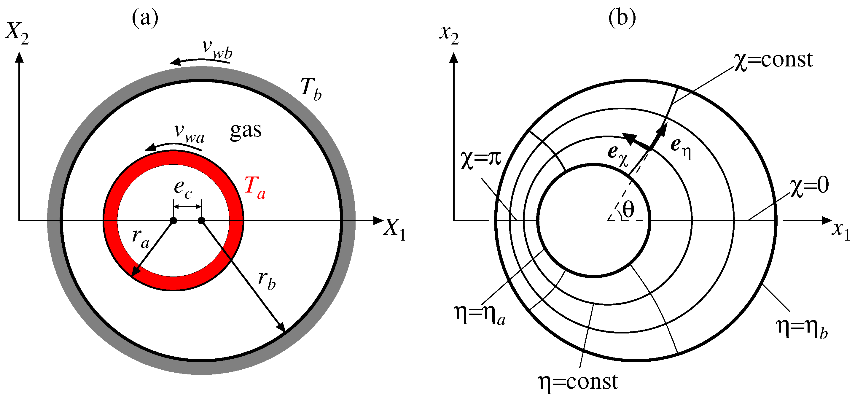
Figure 1. Schematic of the system. (a) Schematic view of the annulus and (b) the bipolar coordinate system ( η , χ ) in the dimensionless space, where x i = X i / ( r b r a ) .
Lubricants 13 00353 g001
Figure 2. Temperature profile at the cross section χ = 0 ( k = 0.1 , c = 0.025 , ε = 0.5 , v ^ w a = 0.1 , v ^ w b = 0 ). (a) Inner heating ( T ^ a = 2 , T ^ b = 1 ) and (b) outer heating ( T ^ a = 1 , T ^ b = 2 ). Solid line for the present solution (46); closed circles for the reference solution [17].
Lubricants 13 00353 g002
Figure 3. Velocity profile at the cross sections χ = 0 and χ = π ( k = 0.1 , c = 0.025 , ε = 0.5 , v ^ w a = 0.1 , v ^ w b = 0 ). (a) Inner heating ( T ^ a = 2 , T ^ b = 1 ) and (b) outer heating ( T ^ a = 1 , T ^ b = 2 ). Solid line for the present solution (51) where v ^ χ = v χ / ( 2 R T 0 ) 1 / 2 = v ^ w u χ ; closed circles for the reference solution and open circles for the unheated case [17].
Lubricants 13 00353 g003
Figure 4. Distribution of the normal stress p ^ η η ( k = 0.1 , c = 0.025 , ε = 0.5 , v ^ w a = 0.1 , v ^ w b = 0 ). (a) Inner heating ( T ^ a = 2 , T ^ b = 1 ) and (b) outer heating ( T ^ a = 1 , T ^ b = 2 ). Solid line for the present solution (62); closed circles for the reference solution and the open circles for the unheated case at y = 0 [17].
Lubricants 13 00353 g004
Figure 5. Magnitude F [Equation (66)] of the eccentric force (41) as a function of the Knudsen number k ( ε = 0.5 , v ^ w a = 0.1 , v ^ w b = 0 ). (a) Inner heating ( T ^ a = 2 , T ^ b = 1 ) and (b) outer heating ( T ^ a = 1 , T ^ b = 2 ). Solid line for the present solution. Closed circles for the reference solution, dotted line for the solution of model B, and the open circles for the unheated case [17].
Lubricants 13 00353 g005
Figure 6. Direction ϑ F [Equation (66)] of the eccentric force (41) as a function of the Knudsen number k ( ε = 0.5 , v ^ w a = 0.1 , v ^ w b = 0 ). (a) Inner heating ( T ^ a = 2 , T ^ b = 1 ) and (b) outer heating ( T ^ a = 1 , T ^ b = 2 ). See the caption of Figure 5.
Lubricants 13 00353 g006
Figure 7. Torque N [Equation (42)] acting on the inner cylinder as a function of the Knudsen number k ( ε = 0.5 , v ^ w a = 0.1 , v ^ w b = 0 ). (a) Inner heating ( T ^ a = 2 , T ^ b = 1 ) and (b) outer heating ( T ^ a = 1 , T ^ b = 2 ). See the caption of Figure 5.
Lubricants 13 00353 g007
Disclaimer/Publisher’s Note: The statements, opinions and data contained in all publications are solely those of the individual author(s) and contributor(s) and not of MDPI and/or the editor(s). MDPI and/or the editor(s) disclaim responsibility for any injury to people or property resulting from any ideas, methods, instructions or products referred to in the content.