Abstract
It has been known for some time that grading of the elastic modulus (namely, softer in the surface) leads to a significant reduction in tensile stresses due to contact loadings; this has been studied mostly to suppress the cracking of brittle materials. In particular, a recent study has demonstrated that the effect is most pronounced for a large Poisson’s ratio, as is the case for incompressible materials. Grading of the modulus occurs intrinsically in viscoelastic materials like rubber when there is a temperature gradient within the rubber, which leads to significant changes of tensile stresses, affecting fatigue and wear. Friction and wear have been analyzed experimentally in the past with respect to mean temperature, revealing an ideal range of temperature with the highest friction and lowest wear, but the effect of the temperature gradient is not as well understood. The present paper presents a simple model of a sinusoidal wave of pressure and shear traction moving on a viscoelastic half-plane (standard material) at constant velocity, finding an approximate solution for a linear variation of viscosity across the depth. We find that tensile stresses may be very significantly altered by temperature changes of a few degrees only across the depth equal to the wavelength of the loading wave. In particular, they are reduced if the temperature decreases with depth, with beneficial effects for fatigue and wear.
1. Introduction
It is known (see Johnson’s book []) that contact loadings induce tensile stresses, particularly in the presence of friction when there is shear traction at the interface like in the case of sliding/rolling. In view of mitigating this effect, Giannakopoulos, Suresh, and co-authors [,,,,,] explored nearly 30 years ago the idea of grading material properties under a static or a sliding contact and found significant beneficial effects against various types of brittle failures due to contact (reduction of “cone” or “herring bone” cracks—which certainly result from high tensile elastic stresses). Recently, Ciavarella and Willert [] presented analytical results for the actual stress field in and below a sliding line contact with an exponentially graded half-plane in the case of sinusoidal pressure and shear, in which case beneficial reduction of tensile stress is particularly significant for high Poisson’s ratios.
In the case of rubber tires, friction and wear both follow “master curves”, as was already demonstrated by Grosch [] and Schallamach [], because both the changes in velocity and temperature affect the viscoelastic properties, as they correspond to changes in loading frequency. However, while friction typically first increases with velocity and then decays (and similarly with temperature), the rate of abrasion typically has the opposite trend: It decays with velocity and then increases before exploding. In any case, the role of tensile stresses in provoking damage and therefore wear by fatigue was demonstrated, and the change in damage at different temperatures was explained by the corresponding change in the material properties of tearing. In other words, the minimum in abrasion is due to a maximum elongation at the break in the material. More recent theories (Persson et al. []) also point to tensile stresses as the cause for a fatigue process, eventually leading to the detachment of particles (wear), although they have not studied the effect of temperature in detail: The effect of the friction coefficient seems to be very strong (a dependence of power 4 or 5), and therefore, it is not trivial to explain why wear decreases exactly where friction increases [].
During tire operation, significant temperature gradients develop across the tire’s thickness due to various factors: (1) frictional heating at the surface; (2) low thermal conductivity of rubber; and (3) internal heat generation (deformation and hysteresis within the tire’s internal structure produce heat, affecting the internal temperature profile).
The performance and durability of rubber tires are critically dependent on the complex interactions between mechanical, thermal, and tribological phenomena occurring at the tire–road interface. The influence of bulk temperature on tire friction and wear has been extensively investigated [], while that on wear is less well understood, and it is well known that there is an “optimal” range of temperature for high friction and low wear, which is why different rubbers are used in different seasons or why in sport competitions, extreme care is taken to reach the optimal range before cars are used. On the other hand, the presence of temperature gradients across the depth of the rubber tread can play a significant role in determining the frictional behavior and wear mechanisms.
Temperature gradients within the tread material affect the viscoelastic properties of rubber dynamically, influencing both the real area of contact and the energy dissipation mechanisms responsible for friction. Furthermore, non-uniform thermal expansion and the associated internal stresses may contribute to the initiation of micro-cracks, accelerating or decelerating fatigue wear (depending on the sign of thermal stresses) and altering the tread’s effective mechanical response. In this paper, we will neglect the role of thermal stresses. For a negative temperature gradient for example, that entails higher temperatures at the surface, leading to expansion which is restrained by lower layers of material; this means that thermal stresses will be compressive and therefore reduce the tendency to fatigue and wear. For a typical road tire compound, the peak friction occurs around 60–90 °C, depending on speed/load, while above 100–120 °C, the friction drops due to excessive softening and potential thermal degradation. The misuse of tires, like using winter tires in summer, exceptional braking, or accelerations, leads to very rapid degradation.
The gradient of temperature across the depth of the tire can be significant, but it depends on a number of factors. During dynamic operation (e.g., rolling, cornering, or braking) the temperature may be complex and time-dependent, and the surface is not always hotter than the inner layers. The surface temperature is influenced by convective cooling (airflow), radiation, and contact time with the road. On the other hand, inner layers, particularly in the tread and carcass, accumulate heat from hysteresis losses due to cyclic deformation and may retain it longer. Also, viscoelastic dissipation may peak internally and cause a temperature peak below the surface, particularly in the tread belt or shoulder area. Given the coupled problem of thermal heat generation and dissipation, viscoelastic deformation and its transient evolution depends on too many factors. Here, we discuss here just as a preliminary step the model of a viscoelastic half-plane loaded by a sinusoidal pressure and a shear traction proportional to pressure (via a friction coefficient) which moves at constant velocity, wherein we consider the effect of a linear gradient of temperature which results in a linear change of viscosity in a standard viscoelastic material. The results show increase/reduction in tensile peak stresses at the interface.
2. Effect of Temperature Gradient on Viscosity
Temperature variation in a viscoelastic body, for instance caused by heat flow from a surface contact, has a significant influence on relaxation or viscosity, as described by the Williams–Landel–Ferry (WLF) equation []. Even simple periodic heat flows in the contact surfaces, e.g., caused by a contact with periodic roughness, lead to relatively complex temperature distributions in the solid (see Ciavarella et al. []). For viscoelastic materials the rate of internal heat generation corresponds to the dissipative part of the mechanical power, i.e., the viscous (inelastic) part, and is given by
with the stress tensor being and the inelastic part of the strain tensor being (a dot denotes derivation in time). This mechanical dissipation induces a temperature field T within the material, which satisfies the steady-state heat conduction equation defined as follows:
where k is the thermal conductivity. Solving the heat equation for the temperature field requires that the associated displacement and hence stress fields must be determined consistently with the mechanical equilibrium equations. If the viscosity is temperature-dependent, these fields are in turn functions of the temperature, making the problem fully thermo-mechanically coupled and analytically intractable. In our work, we will therefore assume a linear temperature profile with depth, as described by the coordinate y pointing into the body:
with the slope a proportional to the heat flow.
Shifts in viscosity due to temperature changes are described in the WLF model via
with the constants , , and determined experimentally. For the viscosity at temperature , we therefore have for the temperature field (3) the depth-dependent viscosity defined as follows:
In order to provide an analytical approximate solution to the subsequent posed problem, we approximate this viscosity by a linear curve, i.e., a first-order Taylor expansion of Equation (5) around :
This enables an investigation of the effect of the grading of viscosity by temperature in contacts using a perturbative approach.
3. Linear Grading of Viscosity—Approximate Solution
We consider now the plane strain problem of a viscoelastic half-plane acted upon by a periodic pressure distribution of amplitude in the normal direction sliding with velocity V (see Figure 1).
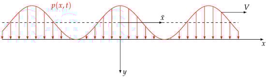
Figure 1.
Periodic sliding pressure acting upon the surface of the viscoelastic half-plane.
At the same time, it is loaded by the stress in the tangential direction, which is related to the pressure distribution through the friction coefficient ; both distributions have the wave number . Their respective values are defined through the following equations:
where the normalized coordinate has been introduced. We are therefore not solving a contact problem in the classical sense; nonetheless, the applied periodic pressure distribution matches a contact problem whose exact surface profile is unknown but certainly wavy in nature—and thus may serve as a reasonable approximation of contact with a rough surface characterized by a single dominant wavelength. But even complex pressure distributions resulting from arbitrary surface shapes may be decomposed into a series of such periodic pressure components examined here.
We assume that through the influence of a temperature gradient, the viscosity is linearly growing with the depth y of the half-plane by the grading coefficient :
From Equation (6), we therefore have
The viscoelastic material shall be rheologically modeled by a standard solid with a modulus in parallel with a series alignment of modulus and viscosity . Therefore, the complex, frequency-dependent modulus G can be written in normalized form as follows:
where the the depth of the half-plane has been normalized with the characteristic length of the problem , and the ratio between the grading coefficient and the wave number has been introduced. The Poisson’s ratio of the material shall be constant in time. The excitation frequency of the material is obviously linked to the sliding velocity: . A full analytical solution of the so posed problem is not possible, as it leads to differential equations with non-constant coefficients. Therefore, we search for a solution through a perturbative approach, which yields good approximate results if and , since the solution will decay exponentially with depth at the rate .
This assumption naturally restricts the temperature gradient a, which—following Equation (9)—can be expressed as a function of the grading coefficient:
As an example, experimental data obtained from a carbon-filled styrene-butadiene rubber can be used [], where , , and . Assuming , for to be of the order 0.5, a maximum temperature gradient of can be analyzed. In the context of using these experimental data, it should be noted that the employed standard material model does not provide a realistic representation of rubber; however, it is sufficient for a qualitative investigation.
The grading coefficient also determines the error made through the assumption of linear change in viscosity, which we can approximate using a Taylor expansion:
If , which will generally be the case, the maximum error over one wavelength is primarily determined by and is approximately . Figure 2 shows the viscosity variation from the WLF model and its linear approximation over the dimensionless depth for the experimental constants mentioned above— and a positive or negative temperature gradient of .
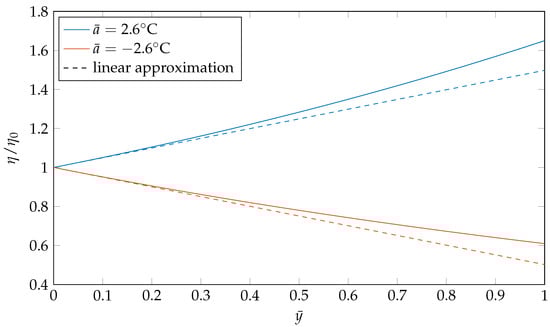
Figure 2.
Viscosity following the WLF model and its linear approximation for a negative or positive temperature gradient as a function of the depth , with , , , .
Returning to the problem at hand, the constant part (in time and space) of the surface loads defined in (7) leads to constant stresses
and therefore, we search for a solution to the non-constant periodic part of the loading. Interpreting (7) as the real part of a complex load, the boundary conditions read as
For a small perturbation , the solution for the displacements of the half-plane will in a first-order approximation have the form
where and are the solutions for the undisturbed case and read as a function of the normalized coordinate :
with the undisturbed complex modulus defined as
Inserting (10), (16) and (17) into the equations for the stresses
and these in turn into the equilibrium equations
one obtains (a prime denotes a derivative with respect to y):
where
The boundary conditions give
With the ansatz
one finds at the same time the homogeneous and particulate solution of (23) and (24) (neglecting terms ), which also satisfies the boundary conditions (26) and (27):
This approximate solution may now be used to determine the stress state occurring in the half-plane as a function of the viscosity grading .
4. Results
Firstly, we consider the case without grading (). Here, the amplitudes of the displacements and thus also of the stresses correspond to the elastic case. This means that the principal stresses and in particular the maximum of the largest principal stress, which we will denote by in the following, also match the elastic case. It is easy to understand that the coefficient of friction plays a major role in this. Without a constant part in the load (that is, and ), the simple relationship
applies. The constant component naturally leads to a reduction in the maximum tensile stress in the material, which now also depends on the Poisson’s ratio. The greater the Poisson’s ratio, the greater this effect as the component in (13) increases. Interestingly, for the case with mean pressure, no closed-form analytical relationship can be given; for the incompressible case however, the following relationship is a good approximation:
Figure 3 shows the course of the normalized maximum principal stress over the coefficient of friction for these different cases.
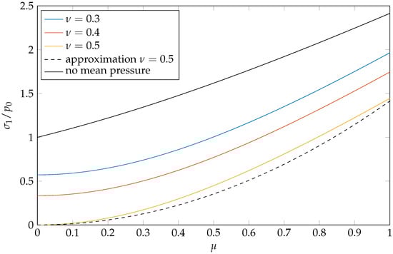
Figure 3.
Maximum principal stress as a function of the friction coefficient for different Poisson’s ratios and the case of no mean pressure, all for no grading.
If grading of the viscosity is introduced, the maximum principal stress now depends, in addition to the grading coefficient, on four parameters: the dimensionless viscosity , the modulus ratio , the friction coefficient , and the Poisson’s ratio . Figure 4 shows, considering mean pressure, the influence of these parameters on the normalized maximum principal stress as a function of the grading coefficient for negative and positive values.
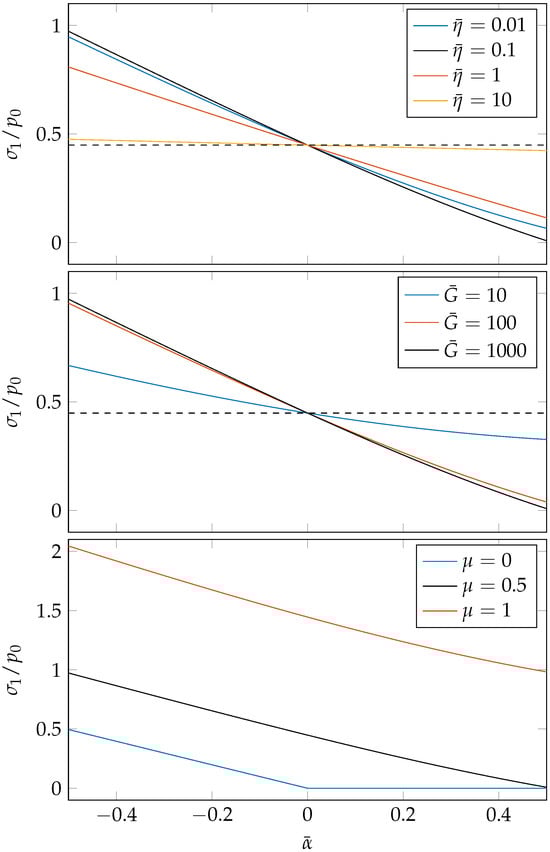
Figure 4.
Normalized maximum principal stress as a function of the grading coefficient varying , , and . Each plot contains in black the reference configuration with , , , and . For better comparison, the dotted line indicates the no-grading level of the reference configuration.
Negative values indicate a rising temperature from the surface into the body (positive gradient), while positive values indicate a decrease in temperature (negative gradient). The first and most significant finding is that a positive gradient in temperature induces an increase in maximum principal stress, while a negative temperature gradient leads to a reduction in principal stresses, with the exception that no decrease occurs below 0. Thereby, the top plots of Figure 4 show that the level of reduction/increase strongly depends on the material parameters and ; to facilitate comparison, the equivalent elastic solution (no grading) is included as a horizontal dashed line. The parameters and have little to no influence on the reduction/increase if the elastic solution () is taken as reference, which itself depends on these parameters. The near-linear progression of the maximum stresses over the presented domain was to be expected given the first-order approximation. Note that the presented solution comes with an error of order , hence being exact for . This means that the rate of change of the maximum principal stress at this point
is also an exact result, i.e., the solution precisely shows how fast maximum tensile stresses are reduced/increased for initial grading. This rate of change is particularly interesting as a function of the parameters and , as the “starting point”, the equivalent elastic solution for no grading, does not depend on them, and thus the rate of change at will give an indication of how far the maximum tensile stresses will reduce or increase also for larger values of —even if the course will probably no longer be linear and approach a limiting value (similar to the results of Ciavarella and Willert [] for the graded elastic material).
Figure 5 and Figure 6 show the normalized rate of change in maximum tensile stresses at as functions of and —with and without mean pressure. Note that the dimensionless viscosity is influenced by the sliding velocity (and the wave number, see (10)), i.e., it increases if the sliding velocity is increased. As is to be expected for very small and very high values of , the influence of grading vanishes, whereas in a mid-range, the rate of change in absolute terms rises to a maximum. The width of the range in which significant rates of change occur and the peak depend on the ratio of the elastic moduli . For a load without mean pressure, there is a slight shift of the distribution in , but more importantly, the maximum rate of change is significantly reduced compared to the case with a constant part in the load, although the largest principal stress itself is higher (see Figure 3). Looking at the rate of change as a function of (Figure 6), small values of lead to no reduction/increase in tensile stresses, since the influence of viscosity in the standard model then vanishes, while the rate of change in absolute terms continuously becomes greater for higher ratios . Here, according to Figure 5, different dimensionless viscosities lead to a shift of the dependency and influence the maximum rate of change that can be reached.
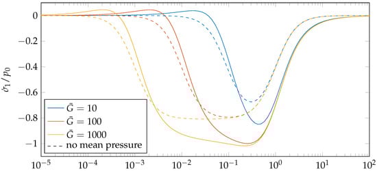
Figure 5.
Rate of change of maximum principal stress for initial grading as a function of the dimensionless viscosity for different values of the parameter , where and .
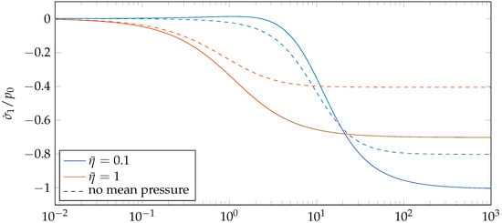
Figure 6.
Rate of change of maximum principal stress for initial grading as a function of the ratio of elastic moduli for different viscosities, where and .
Finally, we shall present a concrete example to show how maximum tensile stresses are reduced for different sliding velocities depending on the wavelength of the external load in order to highlight the influence of these variables hidden in the dimensionless viscosity (Equation (10)). These different wavelengths could, for example, occur as Fourier components of a pressure distribution of a contact with a rough surface. In particular, Persson’s theory [] clarifies that the root mean square (RMS) pressure scales with the RMS slope of the surface and grows unbounded for small wavelengths of roughness.
We again take, for instance, the experimental values of the carbon-filled styrene-butadiene rubber presented above, where , , and . A temperature of shall prevail at the surface and decrease into the body with . This results in a grading coefficient . Furthermore, , and . Figure 7 shows the reduction of the maximum tensile stresses depending on the dimensional wavelength at different sliding velocities.
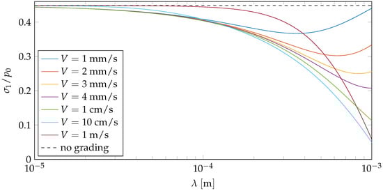
Figure 7.
Maximum tensile stresses as a function of the wavelength of the external load for different sliding velocities, where , , , , .
Note within this example that the presented approximative solution allows for the analysis of relatively high temperature gradients—potentially representative of realistic conditions—for load wavelengths up to the millimeter range resulting, e.g., from a rough surface. It can be seen from Figure 7 that the sliding velocity and wavelength also have a major indirect influence on the reduction of tensile stress via the dimensionless viscosity. According to Figure 5, they therefore also influence the rate of change. In particular, with increasing wavelength, i.e., decreasing dimensionless viscosities, the curve is traversed in the negative direction. This means that the reduction in tensile stresses, which generally increases with increasing wavelength (see Figure 4), is accelerated in an initial phase (Figure 5, right side of the “bell”) and then slowed down or even reversed (left side). The wavelength range at which this happens also depends on the velocity, as it shifts the curve. There is therefore an “optimal” wavelength for which the maximum tensile stresses will be reduced the most; for high velocities, it moves outside the examined wavelength range. It might be explained as follows: Increasing wavelengths cause displacements in a larger area below the surface and are affected by a greater temperature (hence viscosity) difference, but they also lead to a slowing down of the excitation frequency of the viscoelastic material, which ultimately leads to decreasing viscoelastic effects. On the other hand, decreasing viscoelastic effects can also be observed for high velocities and small wavelengths as the excitation frequency becomes very high. Beyond the detailed analysis, it should be noted that over a relatively broad range of velocities, the maximum tensile stresses are significantly reduced, even though there are only a few degrees of temperature change over these wavelengths in the depth of the material.
In the context of wear, Persson’s wear theory [] suggests that the largest wear contribution occurs for an intermediate range of wavelengths, with very small wavelengths contributing little to the total wear loss (although they may be important in the pollution of small particles like PM10 and hence not negligible in this context). Therefore, the effect of temperature gradients will generally alter wear in some specific range of particle dimensions, but not generally the total volume, except for specific conditions where the temperature gradient affects exactly the dominating wavelength range. Since at present, even the effect of mean temperature on wear is also not well understood and captured by theories, the present study cannot give a complete picture, which will require further investigations, particularly as temperature gradients may occur on a small scale as “flash temperatures” where the effects of mean temperature, gradient, but also chemical transformations and the degradation of material properties, will make a realistic model complicated.
5. Conclusions
In this paper, we have shown that in a viscoelastic body loaded at its interface, a temperature gradient along the depth can increase or decrease the maximum tensile stresses. To this end, we have used a perturbative approach to derive an analytical approximate solution for the displacements of a viscoelastic half-plane acted upon by sliding periodic loads in the normal and tangential direction, assuming comparatively small temperature gradients that lead to a approximate linear change in viscosity. The evaluation of the stresses shows that a positive temperature gradient increases the maximum principal stresses in the interface, while a negative gradient reduces them. Although the solution only provides good results for small temperature gradients, it gives—through the rate of change of the maximum principal stresses in this range—an idea of the extent to which maximum stresses can be reduced or increased for higher temperature gradients. Particularly decisive for the increase or reduction in the maximum tensile stress are—for the considered standard solid—the ratios of instantaneous and relaxed moduli, of viscosity and instantaneous modulus, and of the sliding velocity relative to the wavelength of the external load. Even the simple linear perturbative solution presented, derived under the assumption of a standard material model, is sufficient to indicate that in a realistic case a temperature change of just few degrees across a depth equal to the wavelength of the loading wave, gives a dramatic change of peak tension in the surface. Therefore, temperature gradient effects are likely to be important factors in the fatigue and wear of tires. The results of this simple initial study encourage further more detailed analysis of the problem.
Author Contributions
Conceptualization, J.-E.L. and M.C.; methodology, J.-E.L. and M.C.; software, J.-E.L.; validation, J.-E.L. and M.C.; investigation, J.-E.L. and M.C.; writing—original draft preparation, J.-E.L. and M.C.; writing—review and editing, J.-E.L. and M.C.; visualization, J.-E.L.; supervision, M.C. All authors have read and agreed to the published version of the manuscript.
Funding
This research received no external funding.
Data Availability Statement
The datasets generated in this study are available from the corresponding author upon reasonable request.
Acknowledgments
The authors are grateful to Emanuel Willert for originally putting them in touch.
Conflicts of Interest
The authors declare no conflicts of interest.
References
- Johnson, K.L. Contact Mechanics; Cambridge University Press: Cambridge, UK, 1985. [Google Scholar]
- Giannakopoulos, A.E.; Suresh, S. Indentation of solids with gradients in elastic properties: Part I: Point force. Int. J. Solids Struct. 1997, 34, 2357–2392. [Google Scholar] [CrossRef]
- Giannakopoulos, A.E.; Suresh, S. Indentation of solids with gradients in elastic properties: Part II: Axisymmetric indentors. Int. J. Solids Struct. 1997, 34, 2393–2428. [Google Scholar] [CrossRef]
- Suresh, S.; Giannakopoulos, A.E.; Alcalá, J. Spherical indentation of compositionally graded materials: Theory and experiments. Acta Mater. 1997, 45, 1307–1321. [Google Scholar] [CrossRef]
- Jitcharoen, J.; Padture, N.P.; Giannakopoulos, A.E.; Suresh, S. Hertzian-crack suppression in ceramics with elastic-modulus-graded surfaces. J. Am. Ceram. Soc. 1998, 81, 2301–2308. [Google Scholar] [CrossRef]
- Giannakopoulos, A.E.; Pallot, P. Two-dimensional contact analysis of elastic graded materials. J. Mech. Phys. Solids 2000, 48, 1597–1631. [Google Scholar] [CrossRef]
- Suresh, S.; Olsson, M.; Giannakopoulos, A.E.; Padture, N.P.; Jitcharoen, J. Engineering the resistance to sliding-contact damage through controlled gradients in elastic properties at contact surfaces. Acta Mater. 1999, 47, 3915–3926. [Google Scholar] [CrossRef]
- Ciavarella, M.; Willert, E. On the effect of grading elastic modulus in frictional line contacts. J. Tribol. 2025, 147, 071502. [Google Scholar] [CrossRef]
- Grosch, K.A.; Bowden, F.P. The relation between the friction and visco-elastic properties of rubber. Proc. R. Soc. Lond. Ser. A 1963, 274, 21–39. [Google Scholar]
- Schallamach, A. Recent advances in knowledge of rubber friction and tire wear. Rubber Chem. Technol. 1968, 41, 209–244. [Google Scholar] [CrossRef]
- Persson, B.N.J.; Xu, R.; Miyashita, N. Rubber wear: Experiment and theory. J. Chem. Phys. 2025, 162, 074704. [Google Scholar] [CrossRef] [PubMed]
- Williams, M.L.; Landel, R.F.; Ferry, J.D. The temperature dependence of relaxation mechanisms in amorphous polymers and other glass-forming liquids. J. Am. Chem. Soc. 1955, 77, 3701–3707. [Google Scholar] [CrossRef]
- Ciavarella, M.; Decuzzi, P.; Monno, G. Frictionally-excited thermoelastic contact of rough surfaces. Int. J. Mech. Sci. 2000, 42, 1307–1325. [Google Scholar] [CrossRef]
- Xu, R.; Miyashita, N.; Persson, B.N.J. Rubber wear on concrete: Dry and in water conditions. Wear 2025, 578–579, 206200. [Google Scholar] [CrossRef]
- Persson, B.N.J. Theory of rubber friction and contact mechanics. J. Chem. Phys. 2001, 115, 3840–3861. [Google Scholar] [CrossRef]
Disclaimer/Publisher’s Note: The statements, opinions and data contained in all publications are solely those of the individual author(s) and contributor(s) and not of MDPI and/or the editor(s). MDPI and/or the editor(s) disclaim responsibility for any injury to people or property resulting from any ideas, methods, instructions or products referred to in the content. |
© 2025 by the authors. Licensee MDPI, Basel, Switzerland. This article is an open access article distributed under the terms and conditions of the Creative Commons Attribution (CC BY) license (https://creativecommons.org/licenses/by/4.0/).