Machine Tool Spindle Temperature Field Parametric Modeling and Thermal Error Compensation

Abstract

The development of modern machining and manufacturing industry puts forward higher requirements for the machining accuracy of machine tools. The thermal error of the machine tool spindle directly affects the accuracy of the machined workpiece. To improve the accuracy of thermal error prediction, this paper conducts temperature field analysis for the thermal error of the machine tool spindle and employs the Whale Optimization Algorithm (WOA) to optimize the temperature field parameters, aiming to establish a spindle temperature field model. This approach avoids the problem that traditional measurement methods cannot obtain the temperature of key rotational positions of the spindle and provides a new method for the selection of temperature-sensitive points in the thermal error measurement process. Initially, a spindle Product of Exponentials (POE) error model is constructed to map the five errors of the spindle to three-dimensional vectors in the machine tool space. Subsequently, the Whale Optimization Algorithm (WOA) is used to optimize the physical parameters of the spindle, and the optimal spindle temperature field model is determined. The calculated spindle thermal error data and temperature field model data are input into the OLGWO-SHO-CNN model for training. Finally, a case study is carried out on a machining center, and the trained model is used to perform compensation verification under constant and variable speed conditions, respectively. The experimental results show that under the constant speed condition, the compensation rates of the X-axis, Y-axis, and Z-axis are 77.2%, 73.1%, and 88.7%, respectively; under the variable speed condition, the compensation rates of the X-axis, Y-axis, and Z-axis are 74.7%, 78.2%, and 88.0%, respectively. The compensation results indicate that the established spindle temperature field model and the OLGWO-SHO-CNN model have good robustness and accuracy.

1. Introduction

With the development of the modern manufacturing industry, higher requirements have been put forward for the machining accuracy of machine tools. The machining accuracy of machine tools can be improved by preventing or mitigating thermal deformation caused by temperature changes during the machining process, particularly for the spindle, which serves as the core component of precision machine tools [1,2]. The CNC machine tool spindle exhibits key characteristics including a compact structure and high rotational speed. These characteristics, however, contribute to significant heat generation during its rotation, resulting in noticeable thermal deformation in the spindle’s heated regions. Thermal errors in machine tools account for a substantial portion (40–70%) of the total error in actual machining processes [3,4,5]. Moreover, the impact of thermal errors becomes more pronounced as the precision of machine tools increases [6,7]. Thus, it is imperative to adopt effective thermal error compensation or suppression methods to reduce the impact of thermal errors and further improve the machining accuracy of CNC machine tools.

Common error elimination methods can be categorized into two primary types: error prevention and error compensation [8,9,10,11]. Error prevention aims to reduce thermal errors during the machine tool design stage through measures such as symmetrical thermal design, enhanced thermal insulation properties of materials, and active cooling [12,13]. In contrast, surface spray cooling of the spindle or integrating cooling water channels into the spindle can achieve more effective and reliable results in reducing spindle temperature, albeit at the cost of requiring independent hydraulic equipment, a dedicated cooling system, and higher associated costs. Error compensation, on the other hand, involves counteracting generated thermal errors by artificially inducing a displacement of equal magnitude but opposite direction during machine tool operation [14,15,16,17]. Compared to error prevention, error compensation offers lower implementation costs, higher cost-effectiveness, and greater application flexibility.

The error compensation method is typically divided into four key stages: error measurement, temperature measurement point optimization, error modeling, and error compensation [18,19,20]. The purpose of error measurement is to measure the thermal displacement of the spindle in the X, Y, and Z directions within the machine tool workspace, via direct or indirect measurement methods. Common error measurement methods include the three-point method and the five-point method [21,22]. The three-point method can only measure the mixed thermal error resulting from thermal offset and thermal tilt in a single radial direction. This makes it unsuitable for directly measuring thermal offset error, thereby compromising both measurement and compensation accuracy [23,24], and it is rarely used in current practice. On the other hand, the five-point method— which incorporates two extra sensors into the three-point method—enables the measurement of the spindle’s two thermal tilt errors [25,26,27]. Thus, compared with the three-point method, the five-point method is more comprehensive and accurate, and is therefore widely adopted. Although the five-point method can identify five thermal errors, current error compensation methods cannot directly compensate for the two thermal tilt errors—resulting in the spindle’s machining accuracy remaining below the expected level after compensation.

In terms of temperature measurement point optimization, Li et al. [28] proposed a temperature-sensitive point selection method based on feature selection via the improved binary grasshopper optimization algorithm (IBGOA). This algorithm ensures convergence by integrating the optimal approximation criterion into the binary grasshopper optimization algorithm (BGOA). Temperature-sensitive points are then identified based on the cross-validation results of multiple linear regression (MLR). The proposed IBGOA-based feature selection method exhibits more effective clustering performance compared with the traditional fuzzy C-means clustering (FCM)-based temperature-sensitive point selection method. The conventional method for determining temperature-sensitive points relies on temperature and error features and only identifies temperature points that exhibit the same trend as errors; this does not necessarily imply a direct correlation between the errors and the temperature at those points. Spindle thermal errors are typically attributed to frictional heat generated in spindle components, resulting in elevated contact surface temperatures and subsequent spindle thermal deformation, which in turn induces spindle thermal errors. Therefore, when modeling the spindle temperature field, the prevalent approach involves considering heat transfer and frictional mechanisms. Lei et al. [29] proposed a data-driven thermal error model that accurately characterizes the heating behavior of angular contact ball bearings via local heat source analysis of bearing components, elastohydrodynamic lubrication (EHL), and micro-contact theory. Subsequently, they developed a feedback control system to reduce thermal errors to within 1.92 μm. Wu et al. [30] constructed a multi-classification model using a convolutional neural network (CNN) that integrates thermal images and thermocouple data to comprehensively capture spindle temperature field data. Furthermore, Guo et al. [31] employed the grey relational analysis (GRA) method to select temperature variables for thermal error modeling, based on measurement experiments involving spindle heat sources and thermal errors.

The spindle thermal errors can be eliminated via real-time error compensation. To meet the demand for real-time compensation, researchers frequently employ neural network models to establish the mapping relationship between temperature, current, position, velocity, and thermal errors. Lei et al. [32] proposed a closed-loop thermal error compensation system. In this system, an active cooling system was employed as the actuator, and a thermal resistance network was used to develop a physical model that characterizes the combination of heat sources and cold sources. Current thermal error modeling methods primarily rely on temperature data collected from sensors installed at temperature-sensitive points on the spindle. However, a direct correlation is lacking between temperature-sensitive points identified via existing clustering methods and spindle thermal errors. This lack of correlation represents the primary reason for the insufficient robustness of existing thermal error models. Swami Nath Maurya et al. [33] proposed an input attribute optimization model combining artificial neural network prediction and genetic algorithm optimization, with coolant supply temperature, inlet-outlet temperature difference, and flow rate as optimization variables. Within the rotational speed range of 10,000–24,000 rpm, the model achieves a thermal deformation prediction accuracy of 96.26–98.82% for a single spindle. Furthermore, the optimized parameters of the single-spindle system are directly applied to the dual-spindle system, improving the prediction accuracy by 7.31% compared with the variable coolant volume method, while reducing energy consumption by 11–34% and initial investment by 46.5%. Its innovation lies in verifying the feasibility of cross-system reuse of optimized parameters from a single spindle, providing a new idea for low-cost optimization of multi-spindle systems. However, the study still has obvious limitations: the experimental rotational speeds are concentrated in the high-speed range, failing to cover the thermal deformation laws under various rotational speed conditions, which is inconsistent with the actual industrial scenario where spindles often operate in the full range of variable speeds. Although the cooling effect of coolant is mentioned, the influence of lubricant viscosity and temperature sensitivity on frictional heat generation was not quantified. Tria Mariz Arief et al. [34] focused on the monitoring and prediction of the thermo-mechanical behaviors of motorized spindles, constructing an integrated analysis framework combining experimental measurement, multivariate regression, and finite element simulation. They verified a strong correlation between the temperatures at key spindle positions and axial thermal deformation. The proposed four-variable regression model and finite element transient simulation achieved root mean square errors (RMSEs) of 0.84 μm and 0.82 μm, respectively, accurately capturing the time-dependent trend of thermal deformation under different operating conditions. Meanwhile, they optimized the sensor placement scheme, identifying the motor temperature as the optimal sensitive point for single-variable prediction and providing a feasible path for low-cost real-time monitoring. However, the study still has significant gaps: the stability of the model under extreme conditions is unknown; it only verified the measurement effectiveness under steady-state and constant-speed transient conditions, without considering the measurement effectiveness under variable-speed operating conditions; the regression model does not involve a dynamic parameter update mechanism, making it unable to adapt to thermal characteristic drift caused by component aging during long-term spindle operation; it also failed to establish a quantitative relationship between the lubricant viscosity coefficient and bearing frictional heat generation; additionally, the sensor placement scheme does not consider installation space constraints and maintenance costs.

The above research provides valuable theoretical support for further error compensation. However, in terms of temperature measurement point optimization, the conventional approach involves identifying temperature-sensitive points via clustering algorithms and correlation analysis methods. However, this method only identifies temperature curves that closely match the thermal error variation trend and fails to recognize temperature-sensitive points with a direct causal relationship to thermal errors. As a result, the subsequently established prediction model exhibits poor robustness and generalization.

To address the aforementioned issues, this study conducts an analysis of the spindle structure and develops a spindle temperature field model. To begin with, this study measured spindle thermal errors at different rotational speeds using the five-point method. The five identified thermal errors were then mapped to the three-dimensional errors in the machine tool workspace via the product of exponentials (POE) method. Second, this study analyzed the spindle structure and identified temperature-sensitive points to develop the spindle temperature field model. The physical parameters of this model were optimized via the whale optimization algorithm (WOA). Subsequently, the optimized parameters were used to calculate temperatures at the identified temperature-sensitive points. The temperature data at the temperature-sensitive points acquired via the spindle temperature field model exhibited a strong correlation with thermal error data, as thermal errors change in response to temperature variations. Finally, this study trained the proposed OLGWO-SHO-CNN prediction model using error data acquired from measurement and identification, as well as temperature-sensitive point data obtained from measurements and calculations, followed by compensation verification.

This method makes the following contributions: First, by establishing a product of exponentials (POE) model for spindle thermal errors, it addresses the problem of the limited compensation capability of traditional thermal error compensation systems—previously only compensating for thermal offset errors but failing to handle thermal tilt errors. By mapping the five thermal errors to the three directions of the machine tool workspace, the two thermal tilt errors are converted into thermal offset errors within the machine tool workspace. Second, it overcomes the challenge of insufficient correlation between temperature-sensitive point data obtained via existing temperature clustering methods and thermal errors. This goal is achieved by establishing a spindle temperature field model based on the structural characteristics of the spindle, which can acquire temperature-sensitive point data with a strong correlation with thermal errors. While improving the accuracy and robustness of thermal error prediction, this approach reduces the number of sensors required.

The primary objective of this study is to obtain the temperatures at key positions of the spindle that cannot be directly measured by establishing a spindle temperature field model, thereby improving the prediction accuracy of the model. This provides new insights for temperature measurement in subsequent research related to machine tool thermal errors.

2. Principle of Spindle Space Error Identification

2.1. Definition of Spindle Thermal Error

According to the definition specified in ISO 230-3:2020, “Test Code for Machine Tools—Part 3: Determination of Thermal Effects” [35], the main thermal errors of the spindle are primarily composed of the axial thermal elongation error E_ZOC1 (in the Z-direction), along with the radial thermal offset errors E_XOC1 (X-direction) and E_YOC1 (Y-direction). Additionally, the spindle exhibits thermal tilt errors E_AOC1 (about the X-axis) and E_BOC1 (about the Y-axis). The five spindle thermal errors are visualized in Figure 1.

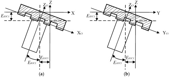
Figure 1. (a) Five thermal errors of the spindle: projection in the XOZ direction. (b) Five thermal errors of the spindle: projection in the YOZ direction.

The element “E” in the error code E_XOC1 is denoted by the letter “E”, while the error direction and type are described by the letter “X”. The error-generating object is represented by the letter “C1”.

2.2. Kinematic Modeling Base on POE

Currently employed compensation methods in three-axis machine tools are limited to addressing thermal offset errors in the X and Y directions, as well as axial thermal elongation errors in the Z direction. However, these methods lack the ability to compensate for thermal tilt errors about the X-axis and Y-axis. In light of this limitation, this study employs the product of exponentials (POE) method to develop a comprehensive kinematic error model. This model enables the mapping of the five primary spindle thermal errors to the X-, Y-, and Z-directions in the machine tool workspace. Consequently, this study established a comprehensive error model within the machine tool workspace.

Equations (1)–(4) below illustrates the combination of the spindle’s five thermal errors to characterize the rotor’s motion—via translation along a specific direction and rotation about the same direction—based on the product of exponentials (POE) theory:

$${\stackrel{\wedge }{\xi }}_{xc1}=\left[\begin{array}{cccccc}{E}_{AOC1}& 0& 0& E_{XOC1}& 0& 0\\ 0& 1& 0& 0& 0& 0\\ 0& 0& 1& 0& 0& 0\\ 0& 0& 0& 1& 0& 0\\ 0& 0& 0& 0& 1& 0\\ 0& 0& 0& 0& 0& 1\end{array}\right]$$

(1)

$${\stackrel{\wedge }{\xi }}_{yc1}=\left[\begin{array}{cccccc}0& E_{BOC1}& 0& 0& E_{YOC1}& 0\\ 0& 1& 0& 0& 0& 0\\ 0& 0& 1& 0& 0& 0\\ 0& 0& 0& 1& 0& 0\\ 0& 0& 0& 0& 1& 0\\ 0& 0& 0& 0& 0& 1\end{array}\right]$$

(2)

$${\stackrel{\wedge }{\xi }}_{zc1}=\left[\begin{array}{cccccc}0& 0& 0& 0& 0& E_{ZOC1}\\ 0& 1& 0& 0& 0& 0\\ 0& 0& 1& 0& 0& 0\\ 0& 0& 0& 1& 0& 0\\ 0& 0& 0& 0& 1& 0\\ 0& 0& 0& 0& 0& 1\end{array}\right]$$

(3)

$$e^{{\stackrel{\wedge }{\xi }}_{c1e}}=e^{{\stackrel{\wedge }{\xi }}_{xc1}}\cdot e^{{\stackrel{\wedge }{\xi }}_{yc1}}\cdot e^{{\stackrel{\wedge }{\xi }}_{zc1}}$$

(4)

where the spindle’s five thermal errors are denoted as E_AOC1, E_BOC1, E_XOC1, E_YOC1, and E_ZOC1. Rotors in the X-, Y-, and Z-directions are represented by ${\stackrel{\wedge }{\xi }}_{xc1}$, ${\stackrel{\wedge }{\xi }}_{yc1}$, and ${\stackrel{\wedge }{\xi }}_{zc1}$, respectively. The product of exponentials (POE) model for the spindle’s error is denoted as ${\mathit{e}}^{{\stackrel{\wedge }{\xi }}_{c1e}}$, while the POE matrices for errors in the X-, Y-, and Z-directions are represented by ${\mathit{e}}^{{\stackrel{\wedge }{\xi }}_{xc1}}$, ${\mathit{e}}^{{\stackrel{\wedge }{\xi }}_{yc1}}$, and ${\mathit{e}}^{{\stackrel{\wedge }{\xi }}_{zc1}}$, respectively.

The multiplication order of the product of exponentials (POE) matrices is determined by the machine tool’s structural characteristics. This study utilized a three-axis vertical milling machine: a fixed coordinate system was placed on the machine tool worktable, and a tool-tip coordinate system was established at the end of the inspection rod clamped in the spindle. Equation (5) illustrates the machine tool’s comprehensive error product of exponentials (POE) model:

$$T_e=e^{-{\stackrel{\wedge }{\xi }}_{xe}}\cdot e^{-S_{xy}{\stackrel{\wedge }{\xi }}_{zi}}\cdot e^{-x{\stackrel{\wedge }{\xi }}_{xs}}\cdot {(e^{-S_{xy}{\stackrel{\wedge }{\xi }}_{zi}})}^{-1}\cdot e^{-{\stackrel{\wedge }{\xi }}_{ye}}\cdot e^{-y{\stackrel{\wedge }{\xi }}_{ys}}\cdot (e^{S_{yz}{\stackrel{\wedge }{\xi }}_{xi}}\cdot e^{-S_{xz}{\stackrel{\wedge }{\xi }}_{yi}})\cdot e^{z{\stackrel{\wedge }{\xi }}_{zs}}\cdot {(e^{S_{yz}{\stackrel{\wedge }{\xi }}_{xi}}\cdot e^{-S_{xz}{\stackrel{\wedge }{\xi }}_{yi}})}^{-1}\cdot e^{{\stackrel{\wedge }{\xi }}_{ze}}\cdot e^{{\stackrel{\wedge }{\xi }}_{c1e}}\cdot e^{{\stackrel{\wedge }{\xi }}_{c1s}}$$

(5)

where the axis-specific error matrices are represented by $e^{-{\stackrel{\wedge }{\xi }}_{xe}}$, $e^{-{\stackrel{\wedge }{\xi }}_{ye}}$, $e^{{\stackrel{\wedge }{\xi }}_{ze}}$, and $e^{{\stackrel{\wedge }{\xi }}_{c1e}}$. Perpendicularity error matrices between the X-, Y-, and Z-axes are denoted by $e^{-S_{xy}{\stackrel{\wedge }{\xi }}_{zi}}$, $e^{S_{yz}{\stackrel{\wedge }{\xi }}_{xi}}$, and $e^{-S_{xz}{\stackrel{\wedge }{\xi }}_{yi}}$. The axis-specific motion matrices are represented by $e^{-x{\stackrel{\wedge }{\xi }}_{xs}}$, $e^{-y{\stackrel{\wedge }{\xi }}_{ys}}$, $e^{z{\stackrel{\wedge }{\xi }}_{zs}}$, and $e^{{\stackrel{\wedge }{\xi }}_{c1s}}$. The machine tool’s comprehensive error matrix is represented by T_e.

Finally, the product of exponentials (POE) model for the spindle thermal errors is presented in Equation (6):

$$\left\{\begin{array}{l}{p}_{ex}=L\cdot E_{BOC1}+E_{XOC1}\hfill \\ p_{ey}=L\cdot E_{AOC1}+E_{YOC1}\hfill \\ P_{ez}=E_{ZOC1}+L\hfill \end{array}\right.$$

(6)

where the spindle’s five thermal errors are represented by E_AOC1, E_BOC1, E_XOC1, E_YOC1, and E_ZOC1. The nominal length of the inspection rod is denoted by L. The spindle’s comprehensive errors in the X-, Y-, and Z-directions within the machine tool workspace are represented by P_ex, P_ey, and P_ez, respectively.

In the modeling process, the nominal length of the inspection rod—denoted as L—was treated as the spindle’s Z-axis motion. It was not subject to compensation and thus omitted from the Z-direction error model.

3. Analysis Model of Heat Transfer Mechanism

3.1. Modelling of Heat Transfer

At different locations within the spindle, various complex heat transfer processes occur during its high-speed rotation. Figure 2 presents an analysis of the heat transfer processes in the spindle structure of the VDL-600A vertical machining center:

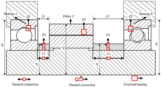
Figure 2. Spindle structure diagram.

The thermal deformations of bearings A, B, and various shaft sections are the primary factors contributing to spindle thermal errors, as these components are highly temperature-sensitive. During high-speed rotation, significant amounts of frictional heat (Q1, Q2, Q3) are generated, resulting from friction between the belt and pulley C, as well as between ball bearings A, B, and their outer rings. As a result, temperatures rise at pulley C and bearings A, B, designating these components as the spindle’s primary heat sources. Temperature at the bearing positions can be measured using temperature sensors mounted on the bearing outer rings. However, due to the spindle’s high rotational speed, it is not feasible to directly measure the temperature at pulley C. Thus, this study developed a spindle temperature field model using heat transfer theory to calculate the temperature at the pulley position.

The heat generated by friction between pulley C and bearings A, B causes a temperature rise in these components. The temperature of bearings A, B is further elevated via heat conduction from the marked shaft segments C1 and C2. The air temperature surrounding the spindle also increases due to heat convection (marked as D1 and D2).

Equation (7) presents the formula for heat generation from friction between pulley C and bearings A, B:

$$\left\{\begin{array}{c}\Delta Q{1}_i={\mu }_1{p}_1{v}_1\\ \Delta Q{2}_i={\mu }_1{p}_2{v}_1\\ \Delta Q{3}_i={\mu }_2{p}_3{v}_2\end{array}\right.$$

(7)

where the frictional heat generation rates for bearings A, B, and pulley C are represented by ΔQ1_i, ΔQ2_i, and ΔQ3_i, respectively. Bearings A and B exhibit a friction coefficient of μ₁, whereas pulley C exhibits a friction coefficient of μ₂. The applied loads on bearings A, B, and pulley C are represented by p₁, p₂, and p₃, respectively. The relative velocity of the frictional surfaces for bearings A and B is denoted as v₁, and the relative velocity of the frictional surfaces for pulley C is denoted as v₂.

Equation (8) presents the formula for heat conduction:

$$\left\{\begin{array}{c}\Delta C{1}_i={\displaystyle \frac{{{\pi d}_3}^2\lambda (T_{Ci}-T_{Ai})}{4L1}}\\ \Delta C{2}_i={\displaystyle \frac{{{\pi d}_3}^2\lambda (T_{Ci}-T_{Bi})}{4L2}}\end{array}\right.$$

(8)

where the heat conduction rates from pulley C to bearings A and B along the spindle shaft are represented as ΔC_1i and ΔC_2i, respectively. The diameter of the heat-conducting shaft segment is denoted as d₃. The thermal conductivity is represented as λ. The instantaneous temperatures of bearings A, B, and pulley C are denoted as T_Ai, T_Bi, and T_Ci, respectively. The axial distances from pulley C to bearings A and B are represented by L1 and L2, respectively.

Equation (9) presents the formula for convective heat transfer:

$$\left\{\begin{array}{c}\Delta D{1}_i=h\pi d_{3}L1(T_{Ci}-T_{hi})\\ \Delta D{2}_i=h\pi d_{3}L2(T_{Ci}-T_{hi})\end{array}\right.$$

(9)

where the convective heat transfer rates between the shaft segments (from pulley C to bearing A, and from pulley C to bearing B) and the surrounding air are represented as ΔD1_i and ΔD2_i, respectively. The convective heat transfer coefficient is denoted as h, whereas the diameter of the heat-conducting shaft segments is represented by d₃. Additionally, the axial distances from pulley C to bearings A and B are represented by L1 and L2. The instantaneous temperatures of pulley C and the spindle’s surrounding air are denoted as T_Ci and T_hi, respectively.

Equation (10) presents the formula for pulley C’s temperature rise and the heat required for this rise:

$$T_{Ci}={\displaystyle \frac{\Delta Q_{xi}}{C\cdot m}}+T_{C(i-1)}$$

(10)

where the instantaneous temperature of pulley C at the current time step is represented by T_Ci, the specific heat capacity of pulley C is denoted as C, the mass of pulley C is represented by m, the heat required for instantaneous temperature rise is denoted as ΔQ_xi, and T_C(i−1) represents the instantaneous temperature at the previous time step.

The heat required for the temperature rise of bearings A and B is provided by conductively transferred heat and friction-induced heat. Heat conduction is the primary contributor to this heat requirement. Considering the complexity of the governing equations, the heat input from bearings A and B’s self-friction (for their temperature rise) is disregarded.

Usually, the instantaneous heat generation of thermal radiation was found to be very small, accounting for less than one percent of the heat generated by friction. Therefore, considering the complexity of the equation, the heat generated by radiation was ignored.

Equation (11) was derived based on the fundamental principle of energy conservation:

$${\displaystyle \sum _{i=1}^n\Delta Q{1}_i+\Delta Q{2}_i+\Delta Q{3}_i-\Delta Q_{xi}}={\displaystyle \sum _{i=1}^n\Delta D{1}_i+\Delta D{2}_i+\Delta C{1}_i+\Delta C{2}_i}$$

(11)

where the frictional heat generation rates of bearings A, B, and pulley C are represented by ΔQ1_i, ΔQ2_i, and ΔQ3_i, respectively. The number of measured temperature points is denoted by n. The heat conduction rates from pulley C to bearings A, B along the spindle shaft are represented by ΔC1_i and ΔC2_i, respectively. Additionally, the convective heat transfer rates between the shaft segments (between pulley C and bearing A, and between pulley C and bearing B) and the surrounding air are represented by ΔD1_i and ΔD2_i, respectively. The heat required for pulley C’s instantaneous temperature rise is denoted by ΔQ_xi.

Equation (12) presents the spindle temperature field model, which was established by substituting Equations (8)–(10) into Equation (11):

$$\begin{array}{l}{\displaystyle \sum _{i=1}^n{\mu }_1{p}_1{v}_1+{\mu }_1{p}_2{v}_1+{\mu }_3{p}_3{v}_2-\Delta Q_{xi}}=\\ {\displaystyle \sum _{i=1}^{n}h\pi d_3(L1+L2)(\frac{\Delta Q_{xi}}{C\cdot m}+T_{C(i-1)}-T_{hi})+}{\displaystyle \frac{{{\pi d}_3}^2\lambda }{4L1L2}}((L1+L2){\displaystyle \frac{\Delta Q_{xi}}{C\cdot m}}+T_{C(i-1)}-L2T_{Ai}-L1T_{Bi})\end{array}$$

(12)

where the friction coefficients of bearings A and B are represented by μ₁, and the friction coefficient of pulley C is represented by μ₂. The number of measured temperature points is denoted by n. The applied loads on bearings A, B, and pulley C are represented by p₁, p₂, and p₃, respectively. The relative velocity of the frictional surfaces of bearings A and B is denoted as v₁, whereas the relative velocity of the frictional surface of pulley C is denoted as v₁. The heat required for instantaneous temperature rise is represented by ΔQ_xi. The convective heat transfer coefficient is denoted as h, and the diameter of the heat-conducting shaft segments is represented by d₃. The axial distances from pulley C to bearings A and B are denoted as L1 and L2, respectively. The instantaneous temperature of pulley C is represented by Tcᵢ, and the instantaneous temperature of the surrounding air at the current time step is represented by T_hi. The specific heat capacity of pulley C is denoted as C, and the mass of pulley C is represented by m. The instantaneous temperature of pulley C at the previous time step is denoted as T_C(i−1), and the thermal conductivity is represented by λ. The instantaneous temperatures of bearings A and B at the current time step are represented by T_Ai and T_Bi, respectively.

The spindle heat transfer model includes numerous material property parameters, many of which can be obtained via measurement or calculation. For instance, the relative velocities of the frictional surfaces (v₁ for bearings A, B; v₂ for pulley C), the diameter of the heat-conducting shaft segments (d₃), and the axial distances from pulley C to bearings A, B (L1, L2) can be directly obtained. However, certain parameters—such as the friction coefficients (μ₁ for bearings A, B; μ₂ for pulley C) and the applied loads on bearings A, B, and pulley C (p₁, p₂, p₃)—are often prone to minor deviations from actual values when obtained via literature research or data lookup. To obtain more precise parameter values, it is customary to use temperature data at specific spindle positions as input, then apply intelligent algorithms to iteratively adjust these parameters and identify values that best match the spindle’s actual operating conditions.

3.2. WOA Optimization Searching

The use of the Whale Optimization Algorithm (WOA) involves simulating various hunting behaviors of whales, including encircling and ensnaring prey, bubble-net feeding, and exploring for food sources. The algorithm employs either random or optimized search agents to emulate these behaviors. WOA has several advantages, including low dependence on tunable parameters and strong global optimization capability. Consequently, WOA is employed to optimize the spindle’s material property parameters.

The algorithm’s specific steps are as follows:

(1)

The population size, maximum number of iterations, and upper/lower bounds for the optimization variables are set. The initial population is randomly generated within these specified bounds;

(2)

The fitness values of the initial population are evaluated by substituting them into the objective function. The population is sorted by the magnitude of fitness values. The position of the individual (in the population) with the minimum fitness value is updated and designated as the optimal solution;

(3)

In the initial stage, whales’ encircling and ensnaring behavior is simulated. The specific formula is given by Equation (13):

$$\left\{\begin{array}{c}D=\left|C*X^{*}(t)-X(t)\right|\\ X(t+1)=X^{*}(t)-A*D\\ A=2a*r_1-a\\ C=2*r_2\end{array}\right.$$

(13)

where the coefficient vectors A and C are used. The current optimal position of an individual in the population is denoted as X*(t), whereas X(t) represents the current position of an individual in the population. The updated position of an individual in the population is represented by X(t + 1). The current iteration number is denoted as t. a is linearly decreased from 2 to 0 over the course of iterations. Random numbers r₁ and r₂ in the range [0, 1] are used. P denotes a random value in [0, 1] that determines either the contraction-expansion mechanism, the spiral motion mechanism, or the prey searching mechanism.

(4)

Whales’ spiral motion behavior during hunting is simulated, and the specific formula is presented in Equation (14):

$$\left\{\begin{array}{ll}X(t+1)=X^{*}(t)+D_p{e}^{bl}\cos (2\pi l)\hfill & ifp<0.5\hfill \\ D_P=X^{*}(t)-A*D\hfill & ifp\ge 0.5\hfill \end{array}\right.$$

(14)

where the distance between a whale and its prey is represented by D_p. The current optimal position of an individual in the population is denoted as X*(t), whereas X(t + 1) represents the updated position of an individual in the population. The spiral shape is denoted by b, while the parameter l is a randomly generated number in the range [−1, 1]. Additionally, the current position of an individual in the population is represented by X(t). The selection of either the contraction–expansion mechanism, the spiral motion mechanism, or the prey searching mechanism is denoted by p, a random value in [0, 1]. Finally, the selection between the spiral motion mechanism and the prey searching mechanism is denoted by A.

(5)

Whales’ prey-searching motion behavior is simulated, and the specific formula is presented in Equation (15):

$$\left\{\begin{array}{l}D=\left|C{X}_{rand}-X(t)\right|\hfill \\ X(t+1)=X_{rand}-A*D\hfill \end{array}\right.ifA>1$$

(15)

where the randomly selected position of an individual whale is represented by X_rand. The current position of an individual in the population is denoted as X(t). A random coefficient vector is denoted by C. The updated position of an individual in the population is represented by X(t + 1). The choice between the contraction-expansion mechanism, the spiral motion mechanism, a random value in [0, 1]. The selection between the spiral motion mechanism or the prey searching mechanism is represented by A.

(6)

Steps (3)–(5) are repeated until the termination condition is satisfied.

3.3. WOA Optimization for Temperature Field Model

The WOA is employed to optimize the physical parameters of the temperature field model. These parameters include the friction coefficients μ₁ (for bearings A, B) and μ₂ (for pulley C), as well as the applied loads p₁ (bearing A), p₂ (bearing B), and p₃ (pulley C). The process flow is shown in Figure 3.

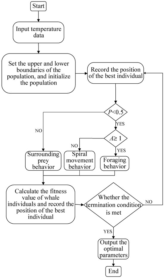
Figure 3. Flow chart of temperature field optimization.

The WOA optimization process for temperature field model parameters is carried out as follows: First, the population size, maximum number of iterations, and upper/lower bounds of the optimization variables for the whale population are set, followed by generating a random initial population whose dimensions match the number of optimization variables. Subsequently, the fitness of each individual in the initial population is calculated by inputting the initial population and measured temperature data into the model, and the optimal individual—corresponding to a smaller residual—is selected based on the highest fitness. A new offspring population is then generated by simulating whale hunting behaviors: encircling prey, spiral movement, and prey searching; after inputting the positions of these offspring individuals into the model to calculate their fitness, the optimal individual (again indicated by the highest fitness and a smaller residual) is chosen. These steps are repeated until the maximum number of iterations is reached.

Through the above three formulas of the Whale Optimization Algorithm (WOA), it is possible to avoid falling into local optimal solutions during the optimization process of the spindle’s physical parameters, making the optimized physical parameters more reasonable.

Through repeated iteration of these steps, the theoretical material parameters in the model gradually converge to the machine tool’s actual state, corrected by input temperature data. Consequently, accurate temperature data at the spindle’s sensitive points can be obtained using the calibrated temperature field model. However, real-time thermal error compensation cannot be achieved solely by obtaining accurate temperature data. To achieve real-time compensation, a reliable mapping between temperature and thermal error must be established. It is worth noting that the fitting performance of mappings established by general mathematical models is poor and lacks robustness and stability. In contrast, neural network models exhibit superior fitting performance, robustness, and stability, as they can effectively establish mappings between complex datasets.

4. Experimental Verification

4.1. Experimental Process

The spindle temperature field model and OLGWO-SHO-CNN model were tested to evaluate their reliability and accuracy. The testing was conducted on the spindle of the VDL-600A CNC vertical machining center, manufactured by Dalian Machine Tool Factory. The test site is shown in Figure 4.

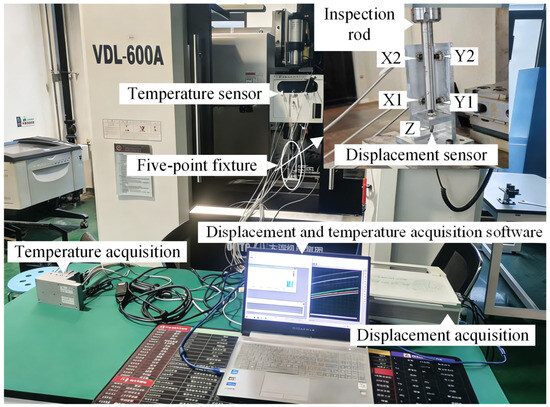
Figure 4. Thermal error test device.

In Figure 4, the Inspection rod refers to the CNC machine tool spindle used to drive the tool for cutting, the Temperature sensor refers to the sensor used to measure the temperature at the temperature-sensitive points of the spindle, the Displacement sensor refers to the sensor used to measure the spindle displacement, the Five-point fixture refers to the special fixture used to fix the Displacement sensor, the Temperature acquisition refers to the data acquisition system used to automatically process the temperature data collected by the Temperature sensor, the Displacement acquisition refers to the data acquisition system used to automatically process the displacement data collected by the Displacement sensor, and the Displacement and temperature acquisition software refers to the software used to display the collected temperature and displacement data and input them into the machine tool for compensation.

The fixture depicted in Figure 4 was securely fastened to the workbench, and a displacement sensor was affixed to a designated position on the fixture using the threaded hole. The TST5910 acquisition system was used to collect displacement data, with an ML-33-02 displacement sensor. For the displacement sensor, the sampling frequency was set to 1 Hz, the measurement range was 2 mm, and the resolution was 0.1 μm. For temperature measurements, the NI-5910 temperature acquisition system was used, paired with a PT100 three-wire platinum resistance temperature sensor. Temperature data were collected at a sampling frequency of 1Hz. When installing the five-point fixture, place the inspection rod on the spindle. The fixture is secured to the workbench using a T-shaped nut. The sensor is fastened in the corresponding position via the threaded hole on the fixture.

Temperature sensors are placed near the upper bearing, lower bearing, and pulley of the spindle. Displacement sensors adopt the five-point measurement method specified in the international standard ISO 230-3:2020 [35] Test Code for Machine Tools—Part 3: Determination of Thermal Effects. During the experiment, both temperature data and thermal displacement data are collected at a frequency of 1 Hz. Before each experiment, the machine tool is left idle for 12 h to ensure it is in a cold state. After sampling and processing, the number of temperature data and thermal error data sets is 16,200.

The travel distances of the machine tool’s X and Y axes are 800 mm, while the Z axis has a travel distance of 500 mm. The maximum feed speed is set to 6000 mm/min. The spindle speed range is 10–10,000 r/min, though long-term operation requires it to be controlled within 8000 r/min. The spindle tool holder model used was BT40, which has a taper ratio of 7:40. The spindle is cooled via water spray. The CNC system used is the Fanuc 0iMATE-TD model, where 0iMATE is the series and TD denotes the specific machining center system version. Before each data acquisition session, the machine tool must be powered off for 10 h. To ensure acquisition system stability, data acquisition for the displacement and temperature systems begins after a 30 min standby period. In the experiments, spindle speeds of 2000 r/min, 5000 r/min, and 8000 r/min were tested, along with variable-speed conditions as shown in the standard variable-speed diagram specified in ISO 230-3. Figure 5 depicts the standard variable-speed diagram used in the experiments.

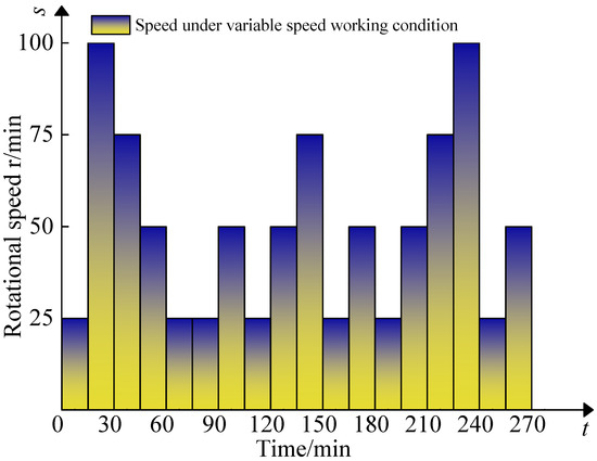
Figure 5. Variable speed map.

4.2. Analysis of Temperature Measurement and Heat Transfer Mechanism of Key Components

Thermal deformation in the machine tool is primarily attributed to heating effects. Heating primarily arises from friction between the inner and outer rings of bearings, between pulleys on the shaft, and between belts. By analyzing the spindle structure discussed in Section 3.1 and constructing a spindle temperature field model, temperature measurements were obtained by positioning sensors near the upper and lower bearings and the pulley. Figure 6 illustrates the placement of these sensors. Table 1 displays the spindle’s structural parameters.

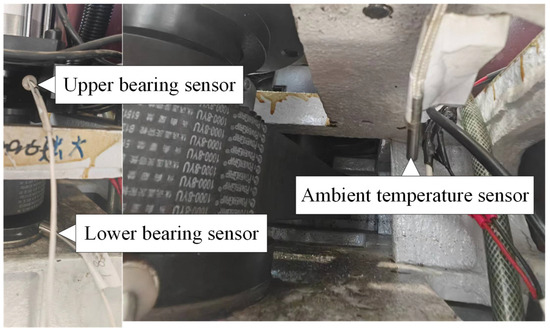
Figure 6. Sensor location.

Table 1. Structural parameters of spindle part.

Parameter	Value
Upper and lower bearing diameter d1	103 mm
Diameter of the pulley d2	138 mm
Shaft diameter d3	75 mm
Distance from the pulley to the lower bearing L1	8 mm
Distance from the pulley to the upper bearing L2	45 mm

The temperature data collected was utilized as input for the spindle temperature field model, followed by the employment of the WOA for optimization purposes. The table presented below illustrates the optimized spindle thermophysical parameters, obtained using temperature data acquired at 8000 r/min. This information was documented in Table 2.

Table 2. Spindle physical parameters.

Parameter	Value
Coefficient of friction for bearings μ1	0.002953
Axial load p1/N	10.0109
Radial load p2/N	94.71056
Coefficient of friction for wheels μ2	0.020022
Load on wheels p3/N	30.0327
Convective heat transfer coefficient h/(W/(m2 °C)	98.27728
Heat capacity ratio for wheels C/(J/(kg·°C))	450.4905
Wheel mass m/kg	8.501093
Thermal conductivity coefficient λ/(W/(m·°C)	10.0109

Through repeated iterations of the above optimization process, the heat required for pulley C’s instantaneous temperature rise—one that best aligns with actual temperature changes—was obtained. Figure 7 presents the heat required for pulley C’s instantaneous temperature rise under optimal physical property parameters.

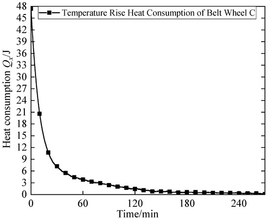
Figure 7. 8000 RPM belt wheel temperature rise consumes heat.

In Figure 7, the instantaneous heat required for pulley C’s temperature rise decreases starting from 48J, and the rate of decrease gradually slows after 120 min.

By substituting the optimized spindle thermophysical parameters into Equation (12) in the spindle temperature field model, the temperature formula for pulley C can be derived, denoted as Equation (16):

$$T_{Ci}=0.998T_{C(i-1)}+8.057\times {10}^{-5}{v}_1+15.653\times {10}^{-5}{v}_2+31.966\times {10}^{-5}{T}_{hi}+143.992\times {10}^{-5}{T}_{Ai}+25.599\times {10}^{-5}{T}_{Bi}$$

(16)

where the current temperature of pulley C is denoted by T_Ci. whereas T_C(i−1) refers to the temperature of pulley C at the previous time step. The rotational linear velocities of bearings A, B, and pulley C are represented as v₁ and v₂, respectively. Additionally, the temperatures near the upper and lower bearings (A and B) and pulley C are denoted by T_ai, T_bi, and T_hi, respectively.

The temperature of pulley C at 8000 r/min was determined by solving Equation (13). Figure 8 displays the temperatures of bearings A, B, and pulley C of the spindle at 8000 r/min.

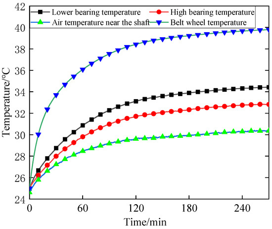
Figure 8. Spindle 8000 RPM bearing and pulley temperature.

In Figure 8, it was observed that the temperature of the lower bearing (bearing B) was higher than that of the upper bearing (bearing A). This difference can be attributed to the lower bearing (bearing B) being closer to pulley C than the upper bearing (bearing A). The analysis in Section 3—based on heat conduction and convective heat transfer principles—indicates that heat conducted from pulley C increases with shorter distances, leading to less heat dissipation during transfer (due to convective effects). In accordance with the principles of temperature rise and heat dissipation, the greater the heat input, the greater the temperature increase. Conversely, the overall temperature near the shaft was the lowest. This can be attributed to convective heat transfer between the surrounding gas and the shaft (near pulley C). This convective heat transfer exhibits a lower heat transfer coefficient and smaller contact area, leading to significantly less heat transfer than heat conduction. When examining the 0–270 min period, it was observed that the temperature at each sensitive point gradually increased. Initially, the temperature increase was rapid, followed by a more stable temperature profile after 120 min. Notably, the temperature variation was most significant at pulley C. This is because sliding friction at pulley C generates considerably more heat than the rolling friction in bearings A and B.

A temperature field model for the spindle rotating at 8000 r/min was established based on Equation (13), and the entire heat variation process is depicted in Figure 9.

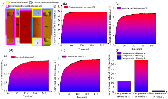
Figure 9. (a) Heat distribution at each part of the spindle structure; (b,c) Heat transfer quantity from pulley C to bearings A and B, respectively; (d,e) Heat transfer quantity between the corresponding shaft segments and the air, respectively; (f) Frictional heat generation quantity of bearings A, B, and pulley C.

In Figure 9, the instantaneous heat conduction rates ΔC1i and ΔC2i (from pulley C to bearings A and B, respectively) are shown in Figure 9b,c. After 60 min, ΔC1i gradually levels off, while ΔC2i levels off after 120 min. The increase in heat transfer rate and magnitude is faster for ΔC1i than for ΔC2i. This is because bearing A is closer to pulley C than bearing B, leading to less heat loss from convection during heat conduction. Consequently, more heat flows to bearing A. In Figure 9d,e, the convective heat transfer between the air and the shaft segments (from pulley C to bearing A, and from pulley C to bearing B) is shown, respectively. The contact area between the shaft segment (pulley C to bearing A) and the air is smaller, as the shorter distance between pulley C and bearing A results in a shorter segment. As a result, the instantaneous convective heat transfer rate is reduced, leading to less heat loss from convection. Figure 9f shows the instantaneous frictional heat generation at bearings A, B, and pulley C, which depends only on load, friction coefficient, and relative sliding/rolling speed. Since the spindle rotates at a constant speed, the instantaneous frictional heat generation remains constant throughout rotation. Due to sliding friction at pulley C—and because the transmission belt is rougher than the metallic surfaces of bearings A and B—the friction coefficient at pulley C is the highest, resulting in the highest instantaneous frictional heat generation there. The highest temperature at pulley C in Figure 9f confirms the above analysis.

4.3. Identification of Thermal Error Measurement for Spindle

Equation (17) presents the identification formula for the five thermal errors.

$$\left\{\begin{array}{l}{E}_{ZO{C}_1}=z\\ E_{AO{C}_1}=(x_1-x_2)/D\\ E_{BO{C}_1}=(y_1-y_2)/D\\ E_{XO{C}_1}=x_1-(L-l)\times E_{AO{C}_1}\\ E_{YO{C}_1}=y_1-(L-l)\times E_{BO{C}_1}\end{array}\right.$$

(17)

In Equation (14): EXOC₁, EYOC₁, EZOC₁, EAOC₁, and EBOC₁ denote the five thermal errors of the spindle; D is the distance between the two displacement sensors on the same side along the axial direction of the spindle; L is the total length of the test bar; l is the distance from sensors X2/Y2 close to the top end of the test bar to the bottom end of the test bar.

The spindle’s thermal displacement data were collected using the five-point fixture and sensors. The collected data were processed using the ICEEMDAN-EWT algorithm, resulting in the processed data shown in Figure 10.

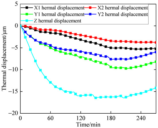
Figure 10. Spindle displacement of 8000 RPM.

In Figure 10, the maximum thermal displacement was observed in the Z-direction, with a peak value of −16.4674 μm. This phenomenon can be attributed to the spindle’s vertical orientation, where gravitational force caused greater thermal deformation in the Z-direction than in the X and Y directions. The second highest thermal displacement was recorded at the Y1 sensor, with a peak value of −9.7541 μm, whereas the Y2 sensor demonstrated a maximum thermal displacement of −7.6495 μm. Moreover, the X1 sensor exhibited a peak thermal displacement of −5.2992 μm, while the X2 sensor indicated the lowest thermal displacement, at only −3.7903 μm.

The results obtained from the five measured thermal displacements—using the spindle spatial thermal error model based on the product of exponentials (PoE), established in Section 2.2—are presented in Figure 11.

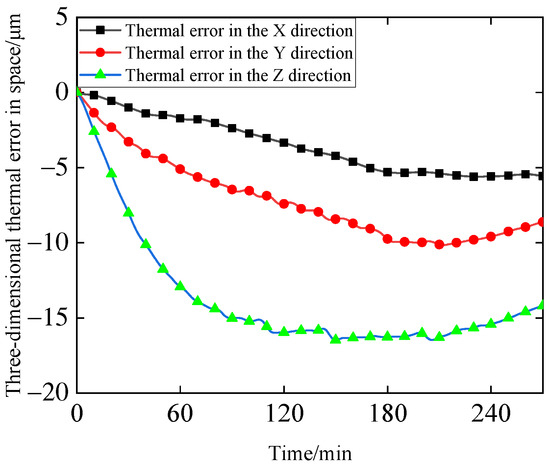
Figure 11. Spindle 8000 RPM space thermal error.

It can be observed in Figure 11 that the Z-axis thermal error exhibits the most significant variation, followed by the Y-axis, and the X-axis thermal error exhibits the least. This phenomenon can be attributed to the spindle’s mechanical structure, where the motor and spindle pulley C are arranged along the Y-axis. When the motor drives pulley C to rotate, a force in the Y-axis direction is exerted on it, resulting in a larger Y-axis thermal error than the X-axis thermal error. Furthermore, the fluctuations observed in the three thermal errors are consistent with temperature changes. Initially, the temperature curve rises rapidly and begins to stabilize after approximately 120 min. Similarly, the thermal error curves initially drop sharply and also level off around the 120 min mark.

4.4. Comparison of Error Compensation Effects

The thermal error data (measured) and temperature data (measured and calculated) were input into the OLGWO-SHO-CNN prediction model for training. The trained model parameters are shown in Table 3.

Table 3. Model parameter.

Parameters	Values
Number of Convolutional Kernels	95
Number of Nodes in the First Fully Connected Layer	143
L2 Regularization Constant	0.000117482
Learning Rate	0.00506

The hyperparameters shown in Table 3 are the optimal ones for model performance, and when the model hyperparameters deviate from the optimal values presented in Table 4, model performance will degrade.

Table 4. Evaluation of the prediction results of each model.

Model	MAE	RMSE	MAPE
OLGWO-SHO-CNN	0.2269	0.3670	3.15%
GA-BP	0.4258	0.5947	5.95%
ISFO-BiLSTM	0.3308	0.4018	4.48%

Three network models, namely OLGWO-SHO-CNN, GA-BP, and ISFO-BiLSTM, are respectively used to predict the identified three-dimensional spatial thermal errors of the spindle. The residuals predicted by each model are evaluated using the mean absolute error (MAE), root mean square error (RMSE), and mean absolute percentage error (MAPE), with the results shown in Table 4.

To verify the accuracy and robustness of the established model, compensation experiments were conducted at a spindle speed of 8000 r/min and under variable-speed conditions. The spatial triaxial thermal errors of the spindle (before and after compensation) are shown in Figure 12 and Figure 13, respectively.

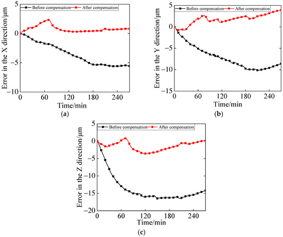
Figure 12. Before and after error compensation in the X, Y, and Z directions at 8000 r/min. (a) Before and after X-direction compensation. (b) Before and after Y-direction compensation. (c) Before and after Z-direction compensation.

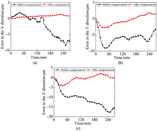
Figure 13. Before and after error compensation in the X, Y, and Z directions at variable speed. (a) Before and after X-direction compensation. (b) Before and after Y-direction compensation. (c) Before and after Z-direction compensation.

Figure 12 illustrates that the X-axis error exhibited the smallest average value after compensation. The errors in the X, Y, and Z directions still exhibited considerable fluctuations after compensation—particularly within the first 120 min. This phenomenon can be attributed to the substantial thermal error variations generated by the spindle within the first 120 min, which subsequently led to notable residual fluctuations even after compensation.

In Figure 13, the X-axis error exhibited the smallest average value after compensation. Prior to compensation, the X-axis error exhibited significant variations but stabilized around 0 μm before the 170th minute. Consequently, the magnitude of the post-compensation error change in the X-direction was noticeably smaller than that in the Y and Z directions. Furthermore, Table 5 and Table 6 present the calculated absolute maximum values, absolute mean values, and error improvement percentages (before and after compensation) for the data in Figure 12 and Figure 13, respectively.

Table 5. Comparison before and after constant speed compensation.

Error Item	The State of Compensation	Absolute Maximum Value/μm	Absolute Average Value/μm	Percentage Improvement
X direction	Before comp.	5.60	3.52	77.2%
	After comp.	2.33	0.80
Y direction	Before comp.	10.15	7.15	73.1%
	After comp.	3.90	1.92
Z direction	Before comp.	16.47	13.7	88.7%
	After comp.	3.59	1.54

Table 6. Comparison before and after variable speed compensation.

Error Item	The State of Compensation	Absolute Maximum Value/μm	Absolute Average Value/μm	Percentage Improvement
X direction	Before comp.	8.42	2.89	74.7
	After comp.	1.32	0.73
Y direction	Before comp.	9.23	6.01	78.2
	After comp.	2.80	1.31
Z direction	Before comp.	17.8	11.09	88.0%
	After comp.	4.27	1.33

Table 5 presents the calculation results, revealing an average Z-axis error of 13.7 μm before constant-speed compensation. This finding indicates that the Z-axis error had the most substantial impact on the CNC machining center over the 270 min operation period. Notably, compensation effectively controlled the average of the spindle’s three-dimensional (3D) spatial errors within 2 μm. After compensation, accuracy improved notably by 77.2%, 73.15%, and 88.7% for the X, Y, and Z axis, respectively.

Similarly, Table 6 reports that the overall 3D spatial errors before variable-speed compensation were relatively smaller than those observed under constant-speed compensation. The Z-axis error—with an average of 11.09 μm—was the most significant of all errors. Compensation significantly mitigated errors: the average of the spindle’s 3D spatial errors was controlled within 2 μm, and accuracy improved by 72.7%, 78.2%, and 88.0% for the X, Y, and Z axes, respectively.

The compensation effect of this study is basically comparable to that of other studies, ranging from 63.50% to 70.27% [36,37].

The above experimental analysis demonstrates that the spindle temperature field model established in this study can accurately calculate the temperature at spindle pulley C. Additionally, the prediction model trained in this study based on the data from the spindle temperature field model and thermal error data can accurately predict the spindle thermal errors.

Based on JJF1059.1-2012 Evaluation and Expression of Measurement Uncertainty and JJG002-2015 Verification Regulation for Temperature Sensors of Automatic Weather Stations the combined standard uncertainties of the eddy current displacement sensors and PT100 platinum resistance temperature sensors are calculated and Table 7 presents the combined standard uncertainties of the relevant measuring instruments.

Table 7. Combined standard uncertainty.

Instrument	Source of Uncertainty	Calculation Formula for Uncertainty	Relative Standard Uncertainty (%)
Eddy Current Displacement Sensor	Uncertainty component introduced by measurement repeatability	Refer to equipment test report	0.13
	Uncertainty introduced by sensor output voltage measurement	$u(e)=\sqrt{{({\displaystyle \frac{0.21\%}{\sqrt{3}}})}^2+{({\displaystyle \frac{{(0.86\%)}^2}{2}})}^2}$	0.12
PT100 Platinum Resistance Temperature Sensor	Uncertainty component introduced by temperature field fluctuation	$u(T)=0.003/\sqrt{3}$	0.20
	Uncertainty component introduced by temperature sensor measurement repeatability	Refer to equipment test report	0.25

By introducing the expansion factor k = 2, the total uncertainty can be obtained as follows:

$$u=k*(0.13\%+u(e)+u(T)+0.25\%)=1.4\%$$

5. Conclusions

In this research, spindle temperature field modeling and thermal error prediction modeling were completed for the spindle of a three-axis vertical milling machine. The following findings were obtained:

(1)

The spindle temperature field model was established by optimizing its thermophysical parameters using the Whale Optimization Algorithm (WOA), resulting in parameters that better reflect the machine tool’s actual operating state. Additionally, incorporating the heat required for instantaneous temperature rise improved the accuracy of the calculated temperature at pulley C.

(2)

Experiments were conducted on a VDL-600A CNC vertical machining center to evaluate the proposed approach’s performance. The results demonstrate that: under constant-speed conditions, compensating for the spindle’s X-axis error reduced the maximum error by 2.27 μm (77.2% precision improvement); compensating for the Y-axis error reduced the maximum error by 6.25 μm (73.1% precision improvement); and compensating for the Z-axis error reduced the maximum error by 12.88 μm (88.7% precision improvement). Under variable-speed conditions, compensating for the X-axis error reduced the maximum error by 7.10 μm (74.7% precision improvement); compensating for the Y-axis error reduced the maximum error by 6.43 μm (78.2% precision improvement); and compensating for the Z-axis error reduced the maximum error by 13.53 μm (88.0% precision improvement).

This study’s experiments did not account for the influence of the spindle’s actual internal structure on the established models. Future work will consider developing a dynamic thermal-mechanical model, which can automatically adjust based on the machine tool’s actual operating state and simulate the machine tool’s entire life cycle to enable predictive analysis.

References

- Dai, Y.; Pang, J.; Rui, X.K.; Li, W.W.; Wang, Q.H.; Li, S.K. Thermal error prediction model of high-speed motorized spindle based on DELM network optimized by weighted mean of vectors algorithm. Case Stud. Therm. Eng. 2023, 47, 15–23. [Google Scholar] [CrossRef]
- Hu, L.; Li, B.H.; Wang, Z.X.; Wang, Y.M. Analysis and evaluation of multi-state wear mechanism of elastic-flexible thin-walled bearings. Tribol. Int. 2025, 202, 110293. [Google Scholar] [CrossRef]
- Hu, L.; Ye, J.; Cui, B.; Wang, Z.X.; Wang, Y.M. Prediction and evaluation of the influence of static-dynamic aging wear of grease on life of high performance bearings (HPBs). Eng. Fail. Anal. 2025, 179, 109829. [Google Scholar] [CrossRef]
- Fu, G.Q.; Zheng, Y.; Lei, G.Q.; Lu, C.J.; Wang, X. Spindle thermal error prediction modeling using vision-based thermal measurement with vision transformer. Measurement 2023, 219, 113272. [Google Scholar] [CrossRef]
- Shi, H.; Qu, Q.Q.; Mei, X.S.; Tao, T.; Wang, H.T. Robust modeling for thermal error of spindle of slant bed lathe based on error decomposition. Case Stud. Therm. Eng. 2023, 51, 103564. [Google Scholar] [CrossRef]
- Dai, Y.; Pang, J.; Li, Z.L.; Li, W.W.; Wang, Q.H.; Li, S.K. Modeling of thermal error electric spindle based on KELM ameliorated by snake optimization. Case Stud. Therm. Eng. 2022, 40, 102504. [Google Scholar] [CrossRef]
- Luo, F.Q.; Ma, C.; Liu, J.L.; Zhang, L.; Wang, S.L. Theoretical and experimental study on rotating heat pipe towards thermal error control of motorized spindle. Int. J. Therm. Sci. 2023, 185, 108095. [Google Scholar] [CrossRef]
- Weng, L.T.; Gao, W.G.; Zhang, D.W.; Huang, T.; Duan, G.L.; Liu, T.; Zheng, Y.J.; Shi, K. Analytical modelling of transient thermal characteristics of precision machine tools and real-time active thermal control method. Int. J. Mach. Tools Manuf. 2023, 186, 104003. [Google Scholar] [CrossRef]
- Fu, G.Q.; Zheng, Y.; Zhou, L.F.; Lu, C.J.; Zhang, L.; Wang, X.; Wang, T. Look-ahead prediction of spindle thermal errors with on-machine measurement and the cubic exponential smoothing-unscented Kalman filtering-based temperature prediction model of the machine tools. Measurement 2023, 210, 112536. [Google Scholar] [CrossRef]
- Wang, G.; Tao, X.S.; Li, Y.; Gao, Y.H.; Dai, Y. Review on thermal error suppression and modeling compensation methods of high-speed motorized spindle. Recent Pat. Eng. 2023, 17, 60–76. [Google Scholar]
- Li, Z.L.; Wang, Q.H.; Zhu, B.; Wang, B.D.; Zhu, W.M.; Dai, Y. Thermal error modeling of high-speed electric spindle based on aquila optimizer optimized least squares support vector machine. Case Stud. Therm. Eng. 2022, 39, 102432. [Google Scholar] [CrossRef]
- Li, Z.L.; Zhu, W.M.; Zhu, B.; Wang, B.D.; Wang, Q.H.; Du, J.M.; Sun, B.C. Simulation analysis model of high-speed motorized spindle structure based on thermal load optimization. Case Stud. Therm. Eng. 2023, 44, 102871. [Google Scholar] [CrossRef]
- Li, Y.; Yu, M.L.; Bai, Y.M.; Hou, Z.Y.; Zhang, H.J.; Wu, W.W. A heat dissipation enhancing method for the high-speed spindle based on heat conductive paths. Adv. Mech. Eng. 2023, 15, 168. [Google Scholar] [CrossRef]
- Hu, L.; Wang, Z.X.; Wang, J.; Wang, Y.M. Derivative Analysis and Evaluation of Roll-slip Fretting Wear Mechanism of Ultra-thin-walled Bearings under High Service. Wear 2024, 11, 205630. [Google Scholar] [CrossRef]
- Wang, L.P.; Kong, X.Y.; Yu, G.; Li, W.T.; Li, M.Y.; Jiang, A.B. Error Estimation and Cross-Coupled Control Based on a Novel Tool Pose Representation Method of a Five-axis Hybrid Machine Tool. Int. J. Mach. Tools Manuf. 2022, 182, 103955. [Google Scholar] [CrossRef]
- Hu, L.; Lee, H.P.; Wang, D.F.; Wang, Z.X. Fatigue Failure of High Precision Spindle Bearing under Extreme Service Conditions. Eng. Fail. Anal. 2024, 25, 158. [Google Scholar] [CrossRef]
- Lai, H.; Pueh, L.; Wang, Z.X.; Wang, Y.M. Surface performance control and evaluation of precision bearing raceway with wireless sensing CBN grinding wheel. Wear 2025, 568, 205966. [Google Scholar]
- Peng, J.; Yin, M.; Cao, L.; Liao, Q.H.; Wang, L.; Yin, G.F. Study on the spindle axial thermal error of a five-axis machining center considering the thermal bending effect. Precis. Eng. 2022, 75, 210–226. [Google Scholar] [CrossRef]
- Gui, H.Q.; Liu, J.L.; Ma, C.; Li, M.Y.; Wang, S.L. Mist-edge-fog-cloud computing system for geometric and thermal error prediction and compensation of worm gear machine tools based on ONT-GCN spatial–temporal model. Mech. Syst. Signal Process. 2023, 184, 109682. [Google Scholar] [CrossRef]
- Li, Y.; Bai, Y.M.; Tian, J.Y.; Zhang, H.J.; Zhao, W.H. Modeling and compensation of the axial thermal error of electric spindles based on HHO-GRU method. Proc. Inst. Mech. Eng. Part B J. Eng. Manuf. 2023, 238, 1815–1826. [Google Scholar] [CrossRef]
- Chiu, Y.; Wang, P.; Hu, Y. The thermal error estimation of the machine tool spindle based on machine learning. Machines 2021, 9, 184. [Google Scholar] [CrossRef]
- Mayr, J.; Egeter, M.; Weikert, S.; Wegener, K. Thermal error compensation of rotary axes and main spindles using cooling power as input parameter. J. Manuf. Syst. 2015, 37 Pt 2, 542–549. [Google Scholar] [CrossRef]
- Zhong, C.B.; Zhuo, M.; Cui, Z.S.; Geng, J.Q. Study on error separation of three-probe method. Symmetry 2022, 14, 866. [Google Scholar] [CrossRef]
- Liu, Y.; Wang, X.F.; Zhu, X.G.; Zhai, Y. Thermal error prediction of motorized spindle for five-axis machining center based on analytical modeling and BP neural network. J. Mech. Sci. Technol. 2021, 35, 281–292. [Google Scholar] [CrossRef]
- Peng, J.; Yin, M.; Cao, L.; Xie, L.F.; Wang, X.J.; Yin, G.F. Study on the thermally induced spindle angular errors of a five-axis CNC machine tool. Adv. Manuf. 2023, 11, 75–92. [Google Scholar] [CrossRef]
- Zhu, M.R.; Yang, Y.; Feng, X.B.; Du, Z.C.; Yang, J.G. Robust modeling method for thermal error of CNC machine tools based on random forest algorithm. J. Intell. Manuf. 2023, 34, 2013–2026. [Google Scholar] [CrossRef]
- Yue, H.T.; Guo, C.G.; Li, Q.; Zhao, L.J.; Hao, G.B. Thermal error modeling of CNC milling machine tool spindle system in load machining: Based on optimal specific cutting energy. J. Braz. Soc. Mech. Sci. Eng. 2020, 42, 456. [Google Scholar] [CrossRef]
- Li, G.L.; Tang, X.D.; Li, Z.Y.; Xu, K.; Li, C.Z. The temperature-sensitive point screening for spindle thermal error modeling based on IBGOA-feature selection. Precis. Eng. 2022, 73, 140–152. [Google Scholar] [CrossRef]
- Lei, M.H.; Yang, J.; Wang, S.; Zhao, L.; Xia, P.; Jiang, G.D.; Mei, X.S. Semi-supervised modeling and compensation for the thermal error of precision feed axes. Int. J. Adv. Manuf. Technol. 2019, 104, 4629–4640. [Google Scholar] [CrossRef]
- Wu, C.Y.; Xiang, S.T.; Xiang, W.S. Spindle thermal error prediction approach based on thermal infrared images: A deep learning method. J. Manuf. Syst. 2021, 59, 67–80. [Google Scholar] [CrossRef]
- Guo, Q.J.; Fan, S.; Xu, R.F.; Cheng, X.; Zhao, G.Y. Spindle thermal error optimization modeling of a five-axis machine tool. Chin. J. Mech. Eng. 2017, 30, 746–753. [Google Scholar] [CrossRef]
- Lei, M.H.; Gao, F.; Li, Y.; Xia, P.; Zhao, L.; Yang, J. Feedback control of the mechanical spindle thermal error based on thermal simulation with bearing heat sources analysis. Proc. Inst. Mech. Eng. Part C J. Mech. Eng. Sci. 2024, 238, 249–263. [Google Scholar] [CrossRef]
- Maurya, S.N.; Luo, W.J.; Panigrahi, B.; Negi, P.; Wang, P.T. Input attribute optimization for thermal deformation of machine-tool spindles using artificial intelligence. J. Intell. Manuf. 2025, 36, 2387–2408. [Google Scholar] [CrossRef]
- Arief, T.M.; Lin, W.Z.; Hung, J.P.; Royandi, M.A.; Chen, Y.J. Monitoring and Prediction of the Real-Time Transient Thermal Mechanical Behaviors of a Motorized Spindle Tool. Lubricants 2025, 13, 269. [Google Scholar] [CrossRef]
- ISO 230-3:2020; Test Code for Machine Tools—Part 3: Determination of Thermal Effects. ISO: Geneva, Switzerland, 2020.
- Liang, Q.K.; Yin, L.; Qiu, C.C.; Zhang, L.J.; Lin, W.C.; Mao, X.Y.; Mao, X. Thermal error prediction of different machine tools based on sequence-to-sequence hybrid domain alignment. Case Stud. Therm. Eng. 2025, 74, 106745. [Google Scholar] [CrossRef]
- Wang, T.X.; Guo, P.; Wang, J.; Mustafa, G.; Meng, X.Z.; Chen, X.S.; Zhang, S. A decoupling modeling method for thermal error prediction of machine tool linear feed axes applicable to cross-conditions. Appl. Therm. Eng. 2026, 283, 128940. [Google Scholar] [CrossRef]
Disclaimer/Publisher’s Note: The statements, opinions and data contained in all publications are solely those of the individual author(s) and contributor(s) and not of MDPI and/or the editor(s). MDPI and/or the editor(s) disclaim responsibility for any injury to people or property resulting from any ideas, methods, instructions or products referred to in the content. |
© 2025 by the authors. Licensee MDPI, Basel, Switzerland. This article is an open access article distributed under the terms and conditions of the Creative Commons Attribution (CC BY) license (https://creativecommons.org/licenses/by/4.0/).