A Deep Learning-Based Model for Recognizing Wear Topography of Self-Lubricating Joint Bearings

Abstract

The study of wear topography in self-lubricating joint bearings is of significant importance for evaluating their service life. In this work, an image dataset was acquired using a white-light interferometer, and the topographical height and color of the images were standardized. Images of worn bearing specimens subjected to 72,000 swing cycles at a frequency of 2 Hz under loads of 100 N, 150 N, 200 N, and 250 N were optimized to construct a processed image dataset. To overcome the limitations of traditional recognition methods in fully capturing both global and local image-based metrics, an improved residual neural network (ResNet) model was proposed. Comparative results with CNN, CapsNet, and conventional ResNet models indicate that, on the processed image dataset, the proposed method improved recognition accuracy by 34% relative to traditional approaches, and by 19% compared to the conventional ResNet. This study provides a novel approach and perspective for investigating the wear topography of self-lubricating joint bearings.

1. Introduction

Self-lubricating spherical plain bearings, also referred to as “industrial joints,” possess advantages such as impact resistance, self-alignment, maintenance-free operation, corrosion resistance, and low cost. Owing to these features, they have gradually become core components in a wide range of fields, including aerospace, marine engineering, the petrochemical industry, rail transit, and large-scale water conservancy and hydropower equipment [1,2,3]. The performance and reliability of such machinery depend largely on the wear life of the bearings [4]. Fundamentally, the bearing wear process manifests as dynamic changes in surface morphology. Consequently, the morphology of the worn surface plays a crucial role in evaluating both the service life and reliability of bearings.

Currently, most research on bearing wear surface morphology follows a three-step approach: data acquisition, feature extraction, and subsequent analysis or prediction of surface morphology parameters [5]. In deep learning research and applications, data acquisition plays a pivotal role in determining model performance and reliability. In recent years, the research paradigm has shifted from being model-centric to data-centric [6], emphasizing that high-quality data fundamentally govern the effectiveness, generalization, fairness, and robustness of deep models [7]. The quality and diversity of collected data define the upper bound of the model’s representational capacity and directly influence its adaptability across domains and demographic groups [8]. Literature suggests that scientific data acquisition should prioritize representativeness, accuracy, and diversity, employing strategies such as active learning, weak supervision, data synthesis, and systematic annotation to improve data coverage and quality [9]. In parallel, engineering practices like data cleaning, validation, and drift monitoring are essential to maintaining long-term model stability and reproducibility [10]. Overall, data acquisition and management have become core components of the deep learning ecosystem, where systematically improving data quality often yields greater performance and trustworthiness gains than further complicating model architectures.

Classical feature extraction methods are generally classified into two categories: signal-based and image-based approaches. In particular, signal-based techniques typically rely on analyses conducted in the time, frequency, and time–frequency domains. In the time domain, indicators are classified into dimensional and dimensionless types. Dimensional indicators include maximum, minimum, median, mean, variance, peak, inter-peak value, and root mean square, while dimensionless indicators include peak factor, margin factor, pulse factor, waveform factor, kurtosis, and skewness [11]. Frequency-domain feature extraction is commonly carried out using Fourier transform (FT), power spectral density (PSD), or spectrum estimation based on autoregressive models (AR). Time–frequency-domain feature extraction combines both time- and frequency-domain analyses and is typically implemented through short-time Fourier transform (STFT), Morlet wavelet (MW), or filter-based Hilbert transform (FHT) [12].

Image-based feature extraction is primarily achieved by scanning and observing the worn surface morphology of bearings using specialized equipment. Commonly employed instruments include scanning electron microscopy (SEM), scanning tunneling microscopy (STM), atomic force microscopy (AFM), transmission electron microscopy (TEM), and white light interferometry (WLI). Typical indicators derived from image-based feature extraction include wear volume, surface roughness, three-dimensional wear morphology, micro-element distribution, and elemental composition of the worn surface [13].

The analysis or prediction of bearing wear surface morphology parameters typically relies on secondary analysis of extracted features and comparison through wear life tests to evaluate bearing performance. However, traditional methods suffer from limitations such as large experimental workload and difficulty in maintaining consistent operating conditions. To address these challenges, researchers have increasingly adopted machine learning and deep learning approaches to identify and predict bearing wear morphology and related parameters. In the field of fault diagnosis, image-based methods have gradually become important tools for detecting faults in bearings and rotating machinery. Studies have shown that bearing faults often manifest as multiplicative changes in signals, causing amplitude scaling or distortion, which can compromise the accuracy of diagnostic algorithms [14,15]. With the development of deep learning techniques, vibration signals or wear data are transformed into two-dimensional representations such as time–frequency spectrograms and texture images, allowing convolutional neural networks (CNNs) to automatically extract deep features and significantly improve fault recognition accuracy and robustness [16,17]. The introduction of image-based features not only enhances the visualization and interpretability of fault patterns but also provides new directions for intelligent diagnosis based on surface morphology or wear texture [18,19]. Furthermore, integrating image recognition techniques with traditional signal analysis and remaining useful life (RUL) prediction offers an effective approach for more comprehensive condition monitoring and life assessment.

Over the past several decades, machine learning algorithms such as decision trees, random forests, k-nearest neighbors, and support vector machines have been widely applied to the study of bearing wear surface morphology. Compared with traditional formula-based methods, these algorithms are capable of modeling nonlinear relationships in a relatively simple manner. More recently, deep learning has emerged as an important branch of machine learning for wear analysis. Deep learning models, including backpropagation neural networks (BP), multilayer Perceptron (MLP), convolutional neural networks (CNN), capsule networks, residual neural networks (ResNet), and hybrid models, employ multi-layer architectures to extract high-level features from complex datasets and to establish nonlinear mappings between input and output variables [20,21].

A number of studies have demonstrated the effectiveness of neural networks in predicting wear-related parameters. Ünlü [22] introduced an artificial neural network (ANN) model to estimate the friction coefficient and wear volume of bearings, achieving an average prediction error of only 1.1%. J.W. et al. [23] applied Latin hypercube sampling to preprocess training data for ANN models, enabling the prediction of viscous and boundary friction values in rolling bearings with a model fit of 99.92%. Edoardo G. et al. [24] developed an ANN for tilt-pad sliding bearings, where backpropagation optimized the network for rapid and accurate prediction of static and dynamic characteristics, outperforming the Reynolds model in both speed and accuracy. Ivan K. et al. [25] used a multilayer perceptron combined with backpropagation to enhance ANN prediction, achieving an accuracy rate of 91.1%.

In the field of bearing wear research, although deep learning methods have achieved significant improvements in the prediction of wear morphology parameters compared with traditional analytical models [26,27], most studies remain focused on quantitative parameter prediction, while holistic image-based analysis of wear morphology is still limited [28,29]. Guo Panpan et al. [30] proposed an enhanced deep convolutional neural network model (IConvNeXt), which constructs datasets from vibration signal images under various fault conditions, achieving 100% recognition accuracy for fault diameters and compound faults, and 99.63% accuracy under variable speeds. Shao Yiping et al. [31] utilized high-resolution measurement technology to obtain 3D point cloud data of worn surfaces and built a spatiotemporal convolutional LSTM model to predict wear height, achieving an average error of only 0.225; the reconstructed point cloud effectively reproduced the next-stage wear morphology, offering a new perspective for wear evolution prediction. She Bo et al. [32] developed a dual-discriminator adversarial domain-adaptive fault diagnosis model that achieved over 99% accuracy across four datasets; however, the approach remains signal-oriented and cannot yet accurately characterize surface morphology. Overall, research on bearing wear morphology is evolving from parameter-based analysis toward image-based deep feature learning and intelligent recognition, yet challenges such as limited high-quality datasets, inconsistent annotations, and complex surface textures persist. Hence, the systematic construction of wear image datasets and end-to-end recognition models represents a key direction for future investigation.

In summary, current research on bearing wear morphology largely focuses on surface morphology parameters or the identification of bearing wear conditions using operational datasets, without directly studying the wear surface morphology images of self-lubricating joint bearings. To address this, the present study standardizes the height coloration of wear surface images and establishes a dataset of self-lubricating joint bearing wear surfaces with uniform height coloring. Convolutional Neural Networks (CNNs), Capsule Neural Networks (CapsNet), Residual Neural Networks (ResNet) are then employed to design and optimize the structures and parameters of wear image recognition models. In order to improve recognition accuracy, a CNN-ResNet recognition model was developed. Finally, comparative experiments are conducted to determine the most suitable model and parameter configuration for recognizing the wear surface morphology of self-lubricating joint bearings. Accurately identifying the wear stages of bearings, especially those approaching failure, enables precise prediction of equipment failure time, thereby effectively reducing machinery failure rates, improving production efficiency, lowering maintenance costs, and extending the service life of the equipment.

2. Preliminaries

2.1. Convolutional Neural Network Algorithm

Convolutional neural network algorithm (CNN) has unique advantages over other deep learning methods in the field of image prediction and recognition due to its advantages of local connection, sharing weighted value, convolution operation and pooling layer.

Since the bearing wear morphology image is two-dimensional, the neuron is usually organized into a three-dimensional neural layer with a size of height (H) × width (L) × depth (D). The convolution kernel in the convolution layer performs convolution operations on the feature map. Since the bearing wear surface morphology is an RGB image with a convolution depth of D = 3. Assuming the bearing wear morphology image A, the size is H × L. And there is a convolution kernel W, with the size of p × q, the formula of the convolution kernel is as follow Equation (1):

$$\mathrm{C}(\mathrm{i},\mathrm{j})=\sum \sum \sum \mathrm{W}(\mathrm{u},\mathrm{v},\mathrm{c})\times \mathrm{A}(\mathrm{i}+\mathrm{u},\mathrm{j}+\mathrm{v},\mathrm{c})$$

(1)

where C (i, j) is the pixel value of the i row and the j column of the convolution operation result, W (u, v, c) is the weighted value of the u row and the v column of the convolution kernel matrix, c represents the color channel of the bearing wear surface morphology (R, G and B values), and A (i + u, j + v, c) is the pixel value in the input image corresponding to the convolution kernel window.

In the process of convolution operation, the convolution kernel needs to perform convolution operations on the color channels (R, G, B) individually of each pixel point. Then the three results of n the color channels (R, G, B) are added. Subsequently output feature mapping is obtained by weighting operation. The specific operation process is shown in Figure 1.

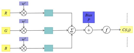
Figure 1. The process of convolution kernel operation.

Input characteristic mapping group of the pooling layer is assumed to be $\mathrm{X}\in {\mathrm{R}}^{\mathrm{H}\times \mathrm{L}\times \mathrm{D}}$. Each feature map $( {\mathrm{X}}^{\mathrm{d}}\in {\mathrm{R}}^{\mathrm{H}\times \mathrm{L}},1\le \mathrm{d}\le \mathrm{D})$ is divided into multiple regions (${\mathrm{R}}_{\mathrm{h},\mathrm{l}}^{\mathrm{d}}$, $1\le \mathrm{h}\le \mathrm{H}$, $1\le \mathrm{l}\le \mathrm{L})$. The pooling function is usually divided into maximum pooling and average pooling. The maximum pooling function is represented by the maximum activity value of all neurons in the maximum pooling selection area ${\mathrm{R}}_{h,\mathrm{l}}^{\mathrm{d}}$. The maximum pooling function is shown as Equation (2), ${\mathrm{x}}_{\mathrm{i}}$ is the activity value of each neuron in ${\mathrm{R}}_{\mathrm{h},\mathrm{l}}^{\mathrm{d}}$.

$$y_{h,l}^d=\underset{i\in R_{h,l}^d}{\max } x_i$$

(2)

Generally, the average activity value of all neurons in the region is taken by the average pooling function, the average pooling function is Equation (3) shown as follow:

$$y_{h,l}^d={\displaystyle \frac{1}{\left|R_{h,l}^d\right|}}{\sum }_{R_{h,l}^d}{x}_i$$

(3)

The output feature mapping Y of the pooling layer is obtained by subsampling each input feature mapping H × L regions, that is, the function formula of Y is as follows Equation (4):

$$Y=\left\{y_{h,l}^d\right\},1\le h\le H,1\le l\le L$$

(4)

When the pooling layer uses a nonlinear activation function, the pooling layer output function W can be expressed as $W=f(wY+b)$, where f(x) is a nonlinear activation function, w and b are learnable scalar weights and biases.

2.2. Residual Neural Network Algorithm and Model

Deeper network models can recognize and predict images by extracting increasingly complex features. However, as network depth increases, the performance of conventional convolutional neural networks often degrades due to issues such as overfitting, underfitting, and vanishing gradients. Residual networks address these challenges by introducing residual connections into nonlinear convolutional layers, thereby improving information propagation. The structure of residual units is illustrated in Figure 2 and Figure 3, where Figure 2 represents a shallow residual unit and Figure 3 a deep residual unit. For a given input x, the convolutional neural network weight layer applies a transformation function F(x). In a residual unit, the original input x is directly added to the transformed output via a skip connection, effectively bypassing the transformation layer to form the residual connection. The residual unit can thus be expressed by Equations (5) and (6).

$$y_1=h\left(x_l\right)+F(x_l,W_l)$$

(5)

$$x_{l+1}=f\left(y_1\right)$$

(6)

Figure 2. The process of shallow residual unit.

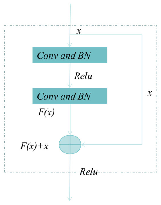
Figure 3. The process of deep residual unit.

${\mathrm{x}}_{\mathrm{l}}$ and ${\mathrm{x}}_{\mathrm{l}+1}$ represent the input and output of the residual unit I, respectively. Each residual unit generally includes a multi-layer structure. F represents the residual function, which represents the learned residual. $h\left({\mathrm{x}}_{\mathrm{l}}\right)$ = ${\mathrm{x}}_{\mathrm{l}}$ represents the identity mapping, and f represents the activation function. Based on the above Formula (6), the learning characteristics from the l layer to the L layer is Equation (7):

$$x_L=x_l+{\sum }_{i=1}^{L-1}F(x_i,W_i)$$

(7)

Using the chain rule, the gradient of the back propagation process can be obtained in Equation (8):

$${\displaystyle \frac{\mathsf{\partial }Loss}{\mathsf{\partial }{x}_l}}={\displaystyle \frac{\mathsf{\partial }Loss}{\mathsf{\partial }{x}_L}}·{\displaystyle \frac{\mathsf{\partial }{x}_L}{\mathsf{\partial }{x}_l}}={\displaystyle \frac{\mathsf{\partial }Loss}{\mathsf{\partial }{x}_L}}·\left(1+{\displaystyle \frac{\mathsf{\partial }}{\mathsf{\partial }{x}_l}}{\sum }_{i=1}^{L-1}F\left(x_i,W_i\right)\right)$$

(8)

where ${\displaystyle \frac{\mathsf{\partial }\mathrm{L}\mathrm{o}\mathrm{s}\mathrm{s}}{\mathsf{\partial }{\mathrm{x}}_{\mathrm{L}}}}$ denotes the gradient of the function to the L layer, and 1 denotes the lossless propagation of the residual element, and preventing gradient vanishing. As shown in Figure 2 and Figure 3, Figure 2 represents a shallow residual unit, while Figure 3 represents a deep residual unit.

2.3. CNN—Residual Neural Network Algorithm and Model

A CNN-ResNet recognition model was developed, consisting of convolutional layers, residual blocks, a fully connected layer, and a classification layer (Figure 4). Initial feature extraction is performed by convolutional layers, with a dropout layer added to reduce overfitting. Four residual blocks, each with two 3 × 3 convolutional layers and skip connections, are then applied to enhance feature learning and gradient transmission. Finally, features are mapped to labels via the fully connected layer. Model parameters are optimized through backpropagation to improve recognition accuracy.

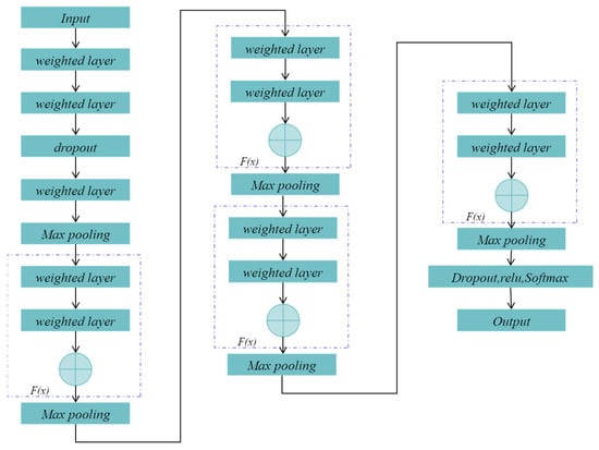
Figure 4. The structure of CNN-ResNet model.

2.4. Capsule Neural Network Algorithm and Model (CapsNet)

The Capsule Neural Network (CapsNet) was proposed to address the limitations of conventional Convolutional Neural Networks (CNNs) in handling images with weak features or partial occlusion [33]. By capturing spatial relationships and pose information among features, CapsNet employs capsule units and a dynamic routing mechanism to effectively represent relative positions and orientations of object parts, thereby enhancing its ability to recognize variations in object pose [34]. Compared with CNNs, CapsNet demonstrates superior generalization, maintaining robust recognition performance under conditions of limited training data or occlusion. Furthermore, its dynamic routing facilitates information exchange across network layers by adaptively adjusting connection weights between capsules, strengthening representational capacity and feature learning. In summary, through capsule units and dynamic routing, CapsNet improves feature learning effectiveness, generalization, and the modeling of spatial relationships [35].

The capsule neural network prediction model consists of an encoder and a decoder. The encoder, composed of capsules, detects specific input features and represents them in vector form. By stacking multiple capsule layers, it captures hierarchical representations and transmits them to the decoder, which reconstructs the input to learn salient features and enable effective classification. The algorithmic framework of CapsNet is illustrated in Figure 5. The input, convolutional, and fully connected layers of a capsule neural network are computed in the same way as in a convolutional neural network, while the capsule layer serves as its core. Each capsule represents a specific feature, and dynamic routing is employed to compute coupling coefficients and update capsule state vectors.

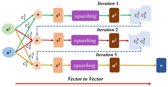
Figure 5. The structure of Capsule Neural Network model.

Dynamic routing is used to compute the coupling coefficient between two capsules, representing their feature similarity, as expressed in Equation (9).

$$c_{ij}={\displaystyle \frac{exp\left(b_{ij}\right)}{\sum _{k}exp\left(b_{ik}\right)}}$$

(9)

Here, $c_{ij}$ denotes the coupling coefficient between capsule i and capsule j, while $b_{ij}$ represents the unnormalized prior coupling coefficient. The term $\sum _{k}exp\left(b_{ik}\right)$ corresponds to the sum of the raw coupling coefficients from capsule i to all capsules j, which is then normalized.

The state vector is updated by aggregating the outputs of child capsules through a weighted sum, as formulated in Equation (10).

$$v_j=Squash({\sum }_i{c}_{ij}·{\widehat{u}}_{j\left|i\right.})$$

(10)

Here, $v_j$ denotes the updated state vector of the parent capsule, and ${\widehat{u}}_{j\left|i\right.}$ represents the output of child capsule i. The squashing function nonlinearly scales the state vector to ensure its length lies between 0 and 1, as defined in Equation (11).

$$Squash(x)={\displaystyle \frac{{‖s‖}^2}{1+{‖s‖}^2}}·{\displaystyle \frac{s}{‖s‖}}$$

(11)

2.5. Image Processing Model

The image processing model is mainly used to process the image of bearing wear surface morphology, and its theoretical principle is based on the PIL module in python 2.0 language. In this study, the image processing functions of the PIL module primarily employed include image opening, saving, and display; mode conversion; channel splitting and merging; cropping, rotation, and resizing; pixel-level manipulations; and conversion to NumPy arrays. The detailed workflow is shown in Figure 6.

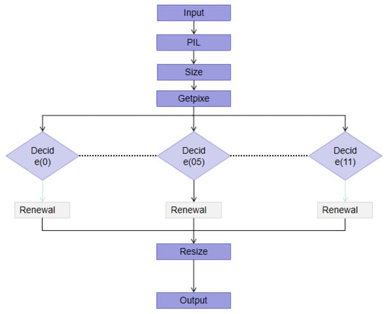
Figure 6. Flow chart of Image processing mode.

The Size function is used to detect image dimensions. Based on the number of pixels, it returns a binary tuple representing width and height, thereby defining the scanning order of the model. The model processes each pixel sequentially, scanning from top to bottom and left to right. The GetPixel function retrieves the RGB values of individual pixels identified by the Size function and outputs them as a NumPy array containing the R, G, and B components. Block recognition is then applied to classify RGB values, ensuring consistent mapping between height information and color representation. In this model, 12 predefined colors are assigned, each corresponding to specific height ranges with defined R, G, and B values. Finally, the Resize function standardizes the processed images to 450 × 300 pixels. Overall, the image processing model unifies both color mapping and pixel dimensions of the bearing wear surface morphology.

3. Experiment and Analysis

3.1. Bearing Wear Testing

In this paper, the friction and wear life test of GE17ES self-lubricating spherical plain bearing is carried out by using the SDZ-50/0.5K low-speed swing wear life tester of China Institute of Aeronautical Technology (Beijing, China) as shown in Figure 7.

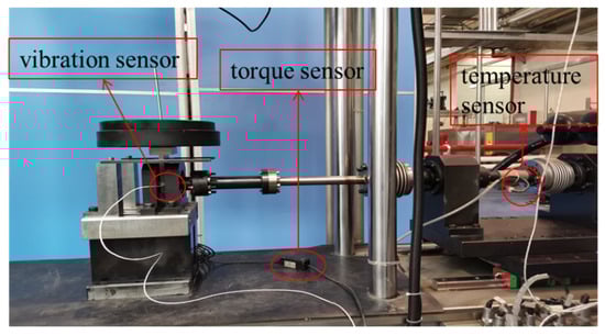
Figure 7. Low speed swing wear life testing machine.

The test bearing is installed in a specific fixture. During the test, the outer ring of the bearing is fixed, and the inner ring rotates with the test machine. The experimental conditions are shown in Table 1. When the friction coefficient of the bearing is higher than 0.1, it is recorded as the wear of the self-lubricating coating of the bearing, that is, the bearing wear is failure. The wear test of the bearing is carried out in the stationary period. When the number of swings reaches 72,000 times (about 10 h), the test is completed.

Table 1. Test scheme of self-lubricating spherical plain bearings.

Number	Frequency	Angle	Force	Times
1–3	2 Hz	±15°	100 N	72,000
4–6	2 Hz	±15°	150 N	72,000
7–9	2 Hz	±15°	200 N	72,000
9–12	2 Hz	±15°	250 N	72,000

The self-lubricating spherical plain bearings was cut by wire cutting equipment after the test as shown in Figure 8. The Bruker Contour GT-K white light interferometer (Bruker corporation, Bremen, Germany) was used to collect the surface topography of the worn bearing slices. Totally 1332 images of the worn surface topography under various working conditions were taken and optimized by Vision 64. The surface topography loaded 100 N is shown in Figure 9 and Figure 10. The wear surface topography under the same working conditions is different, as shown in Figure 10. Therefore, it is necessary to unify the height colors of the wear surface topography image of the self-lubricating spherical plain bearing.

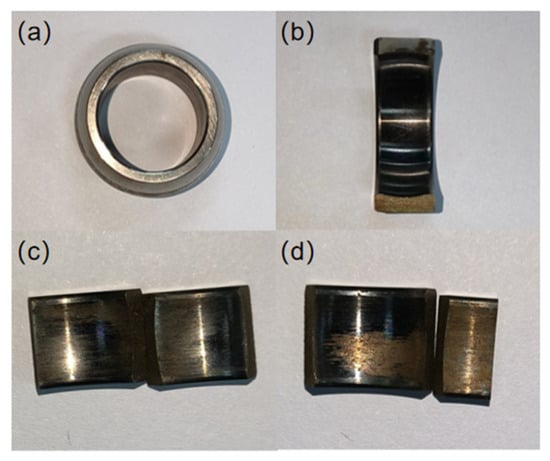
Figure 8. Wear pattern of self-lubricating spherical plain bearings: (a) inner ring, (b) outer ring of unworn area, (c) outer ring of slight worn area, and (d) outer ring of more serious worn area.

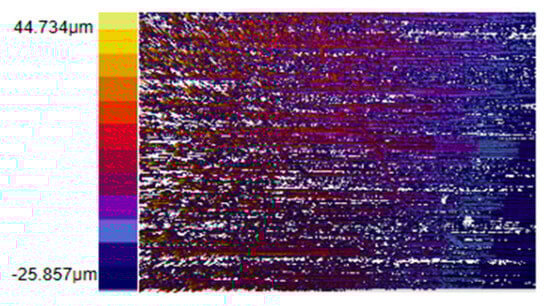
Figure 9. The worn surface topography without optimization by Vision64.

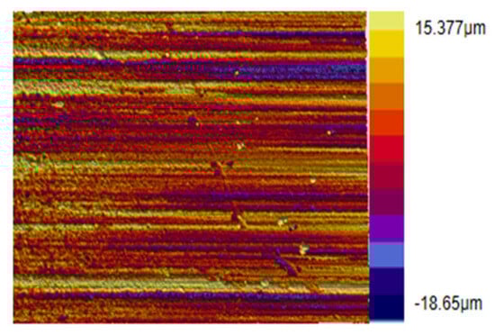
Figure 10. Worn surface topography optimization by Vision64.

3.2. Image Processing Model of Wear Surface Morphology

3.2.1. Wear Image Height Color Division

A total of 1332 images of worn surface morphology were collected under four working conditions. The maximum and minimum height values of each image were analyzed to obtain the corresponding height differences (Figure 11). Based on these values, the images under each condition were classified into three categories: slight wear, moderate wear, and severe wear. Letting A represent the maximum height difference and B the minimum, the recalculated maximum and minimum values are defined by Equations (12) and (13).

$${Max}_i=A-{\displaystyle \frac{(i-1)(A-B)}{12}}$$

(12)

$${Min}_i=A-{\displaystyle \frac{i(A-B)}{12}}$$

(13)

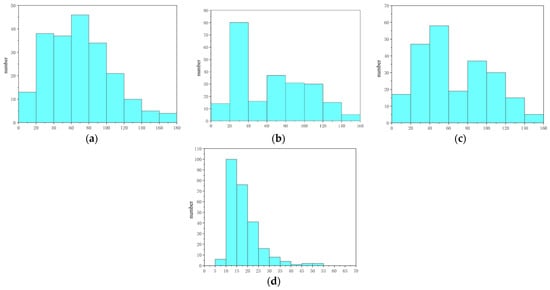
Figure 11. The height difference in wear surface morphology under various working conditions: (a) 100 N, (b) 150 N, (c) 200 N, and (d) 250 N.

Since the wear surface topography image is composed of 12 colors, the height color in the subsequent color bar should be re-build of 6 times. Therefore, it is necessary to make secondary fine-adjustment of Max_A and Max_B again. The height difference color of the wear surface morphology under various working conditions after fine-adjustment is shown in Table 2.

Table 2. Image height values after fine-adjustment under various working conditions.

Load	Slight Worn Images	Moderate Worn Images	Severe Worn Images
100 N	−18 μm~18 μm	−36 μm~36 μm	−66 μm~66 μm
150 N	−12 μm~12 μm	−30 μm~30 μm	−60 μm~60 μm
200 N	−12 μm~12 μm	−24 μm~24 μm	−42 μm~42 μm
250 N	−6 μm~6 μm	−24 μm~24 μm	−18 μm~18 μm

3.2.2. Data Acquisition of Height Color After Fine-Adjustment

To accurately identify the RGB values of the image pixels, the worn surface topography images without Vision64 processing were selected and divided into 12 color regions, as shown in Figure 12 and Table 3. The corresponding RGB values of the color bar are listed in Table 3. Using the Python 2.0 PIL module, the RGB value of each pixel was extracted. For color block No. 1, each row contained 51 columns and 42 pixels, yielding a total of 2142 pixels per intercepted color region. The statistical distributions of the R, G, and B values for this block are presented in Figure 13 and Table 4.

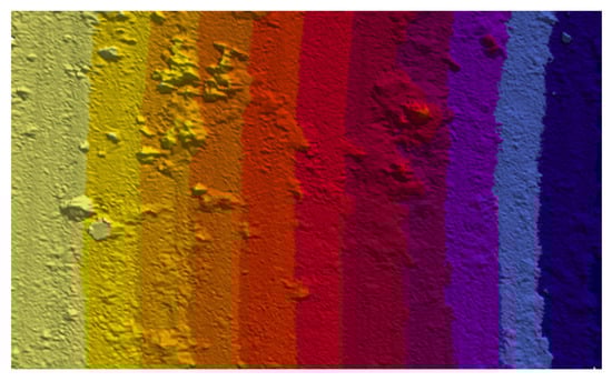
Figure 12. Original worn surface topography with flatting process.

Table 3. The result of divided image.

Number	Color Block	Number	Color Block
1		7
2		8
3		9
4		10
5		11
6		12

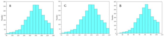
Figure 13. The value of R, G and B about the color No. 1.

Table 4. The value of RGB about each color block.

Color Block	Value of RGB	Color Block	Value of RGB
	R = 232, G = 232, B = 104		R = 160, G = 0, B = 52
	R = 240, G = 208, B = 0		R = 128, G = 0, B = 84
	R = 228, G = 156, B = 0		R = 120, G = 0, B = 172
	R = 216, G = 104, B = 0		R = 80, G = 104, B = 208
	R = 224, G = 52, B = 0		R = 32, G = 0, B = 120
	R = 208, G = 0, B = 36		R = 0, G = 0, B = 96

According to the distribution range of RGB values, the range corresponding to color block No. 1 was first determined. The original image (e.g., Figure 12) was then scanned using the PIL module, and pixels that matched the RGB distribution range of this color block were identified. These pixels were converted to black (R = 0, G = 0, B = 0) for testing, as shown in Figure 14. While most pixels of color block No. 1 were correctly extracted, some remained undetected. To address this, the RGB range of adjacent colors was extracted and subtracted from that of the target color, thereby supplementing the missing pixels until the worn surface morphology appeared as shown in Figure 15. Once the RGB range of a color block could accurately capture all corresponding pixels, the process was terminated. The same procedure was applied to the remaining color blocks, with the finalized RGB values summarized in Table 5.

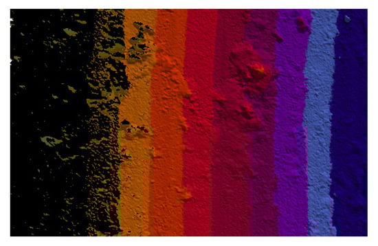
Figure 14. Initially identified worn surface morphology.

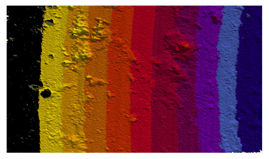
Figure 15. R worn surface morphology removal for No. 1 color.

Table 5. The RGB value range of each color block.

Number	Color	Rang Value of RGB	Number	Color	Rang Value of RGB
1		100 ≤ R ≤ 255, 100 ≤ G ≤ 255, 0 ≤ B ≤ 155	7		65 ≤ R ≤ 156, 0 ≤ G ≤ 0, 29 ≤ B ≤ 57
2		102 ≤ R ≤ 255, 88 < G < 255, 0 ≤ B ≤ 0	8		1 ≤ R ≤ 141, 0 ≤ G ≤ 0, 0 ≤ B ≤ 100
3		34 ≤ R ≤ 222, 55 ≤ G ≤ 155, 0 ≤ B ≤ 0	9		16 ≤ R ≤ 120, 0 ≤ G ≤ 47, 16 ≤ B ≤ 181
4		80 ≤ R ≤ 216, 39 ≤ G ≤ 104, 0 ≤ B ≤ 0	10		35 ≤ R ≤ 119, 31 ≤ G ≤ 155, 91 ≤ B < 255
5		1 ≤ R ≤ 249, 0 ≤ G ≤ 75, 0 ≤ B ≤ 37	11		12 ≤ R ≤ 47, 0 ≤ G ≤ 0, 45 ≤ B ≤ 179
6		0 ≤ R ≤ 208, 0 ≤ G ≤ 0, 0 ≤ B ≤ 57	12		0 ≤ R ≤ 0, 0 ≤ G ≤ 0, 0 ≤ B ≤ 100

3.2.3. Image Dataset of Bearing Worn Surface Morphology

A total of 1332 images were initially obtained by scanning bearing wear slices from top to bottom and left to right using a Bruker Contour GT-K. Some images were excluded due to incomplete or imperfect information, resulting in a final dataset of 1176 images. The dataset was divided at a 6:4 ratio, with 672 images assigned to the training set and 456 to the validation set. Examples of the processed images generated by the proposed image processing model are shown in Table 6. After processing, the surface features of self-lubricating spherical plain bearings appear more complex. Although certain details of the worn topography are not clearly reflected, the color mapping of surface heights is standardized across all images, thereby providing a consistent dataset for analysis. The processed dataset is denoted as AO (After Optimization), while the unprocessed dataset is denoted as BO (Before Optimization).

Table 6. Comparison results of wear surface morphology before and after image processing.

Load	Slight Worn Images		Moderate Worn Images		Severe Worn Images
	BO	AO	BO	AO	BO	AO
100 N
150 N
200 N
250 N

3.3. Comparing the Deep Learning Model

The computer used for running deep learning in this study is equipped with an Intel Core i7-12700 CPU and 48 GB of memory. The deep learning network models developed in this study were implemented using the TensorFlow2.16 library, with a unified coding scheme and input normalization procedure. The labels of worn surface images were encoded using single-hot encoding, as shown in Table 7. Since each worn surface topography image is an RGB three-channel image, its pixel values were normalized by dividing by 255, yielding input dimensions of (450, 300, 3) for the recognition model.

Table 7. Image labels after single-hot encoded processing.

Original Labels	Final Labels	Original Labels	Final Labels
00	[1,0,0,0,0,0,0,0,0,0,0,0]	06	[0,0,0,0,0,0,1,0,0,0,0,0]
01	[0,1,0,0,0,0,0,0,0,0,0,0]	07	[0,0,0,0,0,0,0,1,0,0,0,0]
02	[0,0,1,0,0,0,0,0,0,0,0,0]	08	[0,0,0,0,0,0,0,0,1,0,0,0]
03	[0,0,0,1,0,0,0,0,0,0,0,0]	09	[0,0,0,0,0,0,0,0,0,1,0,0]
04	[0,0,0,0,1,0,0,0,0,0,0,0]	10	[0,0,0,0,0,0,0,0,0,0,1,0]
05	[0,0,0,0,0,1,0,0,0,0,0,0]	11	[0,0,0,0,0,0,0,0,0,0,0,1]

The structural parameters of the image recognition models, including the number of convolutional layers, number of kernels, and kernel sizes, were tested and configured, as these factors directly affect recognition accuracy. In addition, parameters such as the optimizer function, number of iterations, and batch size were optimized and fine-tuned. For the capsule neural network model, parameters including the number of primary capsule layers, capsule layers, convolutional kernels, and kernel sizes were tested and set, while routing iterations, batch size, and total iterations were optimized. The final model parameters are summarized in Table 8.

Table 8. Parameters of deep learning models.

CNN		CapsNet
Name	Parameters	Name	Parameters
Image preprocessing	single-hot coding and data normalization	Image preprocessing	single-hot coding and data normalization
Input layer value	(450, 300, 3)	Input layer value	(450, 300, 3)
convolution layers	12	number of Main capsule and capsule layer	2,6
convolution kernels	16 + 2n	convolution kernels	16 + 2n
Convolution kernel size	(3 × 3)	Convolution kernel size	(3 × 3)
Model optimizer	Adam	Route iteration times	5
iterations	60	batch samples	12
batch samples	6	iterations	60

3.4. Analysis

Based on the BO and AO image datasets, four models—CNN–ResNet, CNN, CapsNet, and ResNet—were trained and evaluated, with the validation set used for performance verification. Figure 16, Figure 17, Figure 18 and Figure 19 present the loss and accuracy values for both the training and validation sets. When using the AO dataset, all models achieved significant improvements compared with the BO dataset. For the training set, the loss values of CNN–ResNet, CNN, CapsNet, and ResNet decreased by 3.67, 13.31, 1.52, and 4.83, respectively, while recognition accuracy increased by 4%, 2%, 3%, and 5%. For the validation set, the loss values of the four models were reduced by 56.69, 30.97, 27.72, and 32.45, with accuracy improvements of 34%, 21%, 28%, and 25%, respectively.

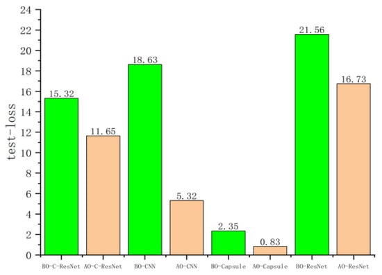
Figure 16. The loss value of the worn image recognition model on training set.

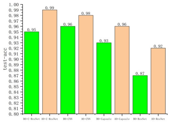
Figure 17. The accuracy value of the worn image recognition model on training set.

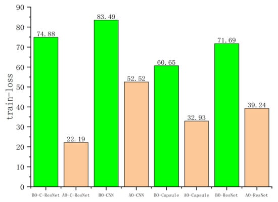
Figure 18. The loss value of the worn image recognition model on verification set.

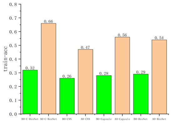
Figure 19. The accuracy value of the worn image recognition model on verification set.

Although the improvements in the training set were relatively modest—likely due to the limited dataset size and the relatively deep network architectures—the gains on the validation set were substantial. Notably, CNN–ResNet achieved the highest improvement, with validation accuracy increasing by 34%.

In conclusion, the proposed image processing model for worn surface topography of self-lubricating spherical plain bearings not only unifies surface height and color representations but also significantly enhances the performance of deep learning recognition models.

To evaluate the performance of the proposed CNN–ResNet model, a comprehensive comparison was conducted with CNN, CapsNet, and ResNet in terms of training time, coefficient of determination (R²), loss values, and accuracy during both training and validation. The results are summarized in Table 9. Compared with CNN, CapsNet, and ResNet, the R² values of CNN–ResNet improved by 0.31, 0.15, and 0.21, respectively. Training set accuracy increased by 1%, 4%, and 7%, while validation set accuracy improved by 19%, 10%, and 12%. However, the training time increased by 4 h, 2.2 h, and 0.2 h, respectively. Overall, the CNN–ResNet model demonstrates superior recognition performance for worn surface images, showing substantial improvements across multiple metrics compared with ResNet, albeit with a modest increase in training time.

Table 9. The evaluation results of the four models.

Models	Training Time	R2	Test-Loss	Test-Acc	Train-Acc	Train-Loss
CNN-ResNet	8.1 h	0.77	11.65	0.99	0.66	22.19
CNN	4.1 h	0.46	5.32	0.98	0.47	52.52
CapsNet	6.3 h	0.62	0.83	0.96	0.56	32.93
ResNet	7.9 h	0.56	16.73	0.92	0.54	39.24

4. Conclusions

The wear surface morphology serves as a critical indicator for investigating the service life and reliability of bearings. By employing deep learning algorithms to characterize the wear surface morphology and determine the corresponding operational stage, the remaining service life of the bearing can be effectively predicted.

This study establishes an image recognition framework for bearing wear morphology that unifies inconsistent height–color mapping. By introducing an improved residual neural network, the model automatically extracts image-based metrics and reduces the influence of chromatic aberration. Compared with the CNN, CapsNet, and ResNet models, the CNN–ResNet network model demonstrates improvements in the coefficient of determination of 0.31, 0.15, and 0.21, respectively. The model’s accuracy on the training set increases by 1%, 4%, and 7%, while its accuracy on the validation set is enhanced by 19%, 10%, and 12%, respectively. The CNN–ResNet network model achieves superior performance and can address most issues related to workpiece surface morphology images and also provides a new approach for studying bearing wear life.

References

- Zhang, Q.; Hao, C.; Wang, Y.; Zhang, K.; Yan, H.; Lv, Z.; Fan, Q.; Xu, C.; Xu, L.; Wen, Z.; et al. Intelligent fault diagnosis of rotating machinery based on improved hybrid dilated convolution network for unbalanced samples. Sci. Rep. 2025, 15, 14127. [Google Scholar] [CrossRef]
- Hakim, M.; Omran, A.A.B.; Ahmed, A.N.; Al-Waily, M.; Abdellatif, A. A systematic review of rolling bearing fault diagnoses based on deep learning and transfer learning: Taxonomy, overview, application, open challenges, weaknesses and recommendations. Ain Shams Eng. J. 2023, 14, 101945. [Google Scholar] [CrossRef]
- Wu, G.; Yan, T.; Yang, G.; Chai, H.; Cao, C. A Review on Rolling Bearing Fault Signal Detection Methods Based on Different Sensors. Sensors 2022, 22, 8330. [Google Scholar] [CrossRef]
- Althubaiti, A.; Elasha, F.; Teixeira, J.A. Fault diagnosis and health management of bearings in rotating equipment based on vibration analysis—A review. J. Vibroeng. 2021, 24, 46–74. [Google Scholar] [CrossRef]
- Xu, J. Research on Bearing Surface Defect Detection and Classification Method Based on Deep Learning. Master’s Thesis, Zhengzhou University, Zhengzhou, China, 2022. (In Chinese). [Google Scholar]
- Roh, Y.; Heo, G.; Whang, S.E. A survey on data collection for machine learning: A big data—AI Integration perspective. IEEE Trans. Knowl. Data Eng. 2021, 33, 1328–1347. [Google Scholar] [CrossRef]
- Whang, S.E.; Roh, Y.; Song, H.; Lee, K. Data collection and quality challenges in deep learning: A data-centric AI perspective. VLDB J. 2023, 32, 791–813. [Google Scholar] [CrossRef]
- Gong, Y.; Liu, G.; Xue, Y.; Li, R.; Meng, L. A survey on dataset quality in machine learning. Inf. Softw. Technol. 2023, 162, 107268. [Google Scholar] [CrossRef]
- Zhou, Y.; Wang, H.; Xu, K. A Survey on data quality dimensions and tools for machine Learning. arXiv 2024, arXiv:2406.19614. [Google Scholar] [CrossRef]
- De, S.; Moss, H.; Johnson, J.; Li, J.; Pereira, H.; Jabbari, S. Engineering a machine learning pipeline for automating metadata extraction from longitudinal survey questionnaires. IASSIST Q. 2022, 46, 1–12. [Google Scholar] [CrossRef]
- Cascales-Fulgencio, D.; Quiles-Cucarella, E.; García-Moreno, E. Computation and statistical analysis of bearings’ time- and frequency-domain features enhanced using cepstrum pre-whitening: A ML- and DL-based classification. Appl. Sci. 2022, 12, 10882. [Google Scholar] [CrossRef]
- Aasi, A.; Tabatabaei, R.; Aasi, E.; Jafari, S.M. Experimental investigation on time-domain features in the diagnosis of rolling element bearings by acoustic emission. J. Vib. Control 2021, 28, 2585–2595. [Google Scholar] [CrossRef]
- Hoang, D.; Kang, H. A survey on Deep Learning based bearing fault diagnosis. Neurocomputing 2019, 335, 327–335. [Google Scholar] [CrossRef]
- Peng, H.; Zhang, H.; Fan, Y.; Shangguan, L.; Yang, Y. A review of research on wind turbine bearings’ failure analysis and fault diagnosis. Lubricants 2023, 11, 14. [Google Scholar] [CrossRef]
- Kumar, P.; Tiwari, R. A review: Multiplicative faults and model-based condition monitoring strategies for fault diagnosis in rotary machines. J. Braz. Soc. Mech. Sci. Eng. 2023, 45, 282. [Google Scholar] [CrossRef]
- Wang, L.; Zhang, X.; Miao, Q. Understanding theories and methods on fault diagnosis for multi-fault detection of planetary gears. In Proceedings of the 2016 Prognostics and System Health Management Conference (PHM-Chengdu), Chengdu, China, 19–21 October 2016; pp. 1–8. [Google Scholar] [CrossRef]
- Chen, C.; Mo, C. A method for intelligent fault diagnosis of rotating machinery. Digit. Signal Process. 2004, 14, 203–217. [Google Scholar] [CrossRef]
- Wang, Y.; Zhao, Y.; Addepalli, S. Remaining useful life prediction using deep learning approaches: A review. Procedia Manuf. 2020, 49, 81–88. [Google Scholar] [CrossRef]
- Chen, Y.; Zhang, T.; Luo, Z.; Sun, K. A Novel Rolling Bearing Fault Diagnosis and Severity Analysis Method. Appl. Sci. 2019, 9, 2356. [Google Scholar] [CrossRef]
- Anwarsha, A.; Babu, T.N. Recent advancements of signal processing and artificial intelligence in the fault detection of rolling element bearings: A review. J. Vibroeng. 2022, 24, 1027–1055. [Google Scholar] [CrossRef]
- Zhang, S.; Zhang, S.; Wang, B.; Habetler, T.G. Deep learning algorithms for bearing fault diagnostics—A comprehensive review. IEEE Access 2020, 8, 29857–29881. [Google Scholar] [CrossRef]
- Sadık Ünlü, B.; Durmuş, H.; Meriç, C. Determination of tribological properties at CuSn10 alloy journal bearings by experimental and means of artificial neural networks method. Ind. Lubr. Tribol. 2012, 64, 258–264. [Google Scholar] [CrossRef]
- Walker, J.; Questa, H.; Raman, A.; Ahmed, M.; Mohammadpour, M.; Bewsher, S.R.; Offner, G. Application of tribological artificial neural networks in machine elements. Tribol. Lett. 2023, 71, 3. [Google Scholar] [CrossRef]
- Gheller, E.; Chatterton, S.; Panara, D.; Turini, G.; Pennacchi, P. Artificial neural network for tilting pad journal bearing characterization. Tribol. Int. 2023, 188, 108833. [Google Scholar] [CrossRef]
- Knežević, I.; Rackov, M.; Kanović, Ž.; Buljević, A.; Antić, A.; Tica, M.; Živković, A. An analysis of the influence of surface roughness and clearance on the dynamic behavior of deep groove ball bearings using artificial neural networks. Materials 2023, 16, 3529. [Google Scholar] [CrossRef]
- Wang, Q.; Wang, X.; Zhang, X. Tribological properties study and prediction of PTFE composites based on experiments and machine learning. Tribol. Int. 2023, 188, 108815. [Google Scholar] [CrossRef]
- Podsiadlo, P.; Stachowiak, G.W. Development of advanced quantitative analysis methods for wear particle characterization and classification to aid tribological system diagnosis. Tribol. Int. 2005, 38, 887–897. [Google Scholar] [CrossRef]
- Wen, S.; Chen, Z.; Li, C. Vision-Based Surface Inspection System for Bearing Rollers Using Convolutional Neural Networks. Appl. Sci. 2018, 8, 2565. [Google Scholar] [CrossRef]
- Que, H.; Liu, X.; Jin, S.; Huo, Y.; Wu, C.; Ding, C.; Zhu, Z. Partial Transfer learning method based on Inter-Class feature transfer for rolling bearing fault diagnosis. Sensors 2024, 24, 5165. [Google Scholar] [CrossRef] [PubMed]
- Guo, P.; Zhang, W.; Cui, B.; Guo, Z.; Zhao, C.; Yin, Z.; Liu, B. Multi-condition fault diagnosis method of rolling bearing based on enhanced deep convolutional neural network. J. Vib. Eng. 2025, 38, 96–108. (In Chinese) [Google Scholar]
- Shao, Y.; Tan, J.; Lu, J. A spatio-temporal fully convolutional recurrent neural network based surface topography Prediction. J. Mech. Eng. 2021, 57, 292–304. (In Chinese) [Google Scholar]
- She, B.; Liang, W.; Qin, F.; Dong, H. Open set domain adaptation method based on adversarial dual classifiers for fault diagnosis. Chin. J. Sci. Instrum. 2023, 44, 325–334. (In Chinese) [Google Scholar]
- Chen, T.; Wang, Z.; Yang, X.; Jiang, K. A deep capsule neural network with stochastic delta rule for bearing fault diagnosis on raw vibration signals. Measurement 2019, 148, 106857. [Google Scholar] [CrossRef]
- Zhu, Z.; Peng, G.; Chen, Y.; Gao, H. A convolutional neural network based on a capsule network with strong generalization for bearing fault diagnosis. Neurocomputing 2019, 323, 62–75. [Google Scholar] [CrossRef]
- Zhao, X.; Chai, J. Adaptive weight-based capsule neural network for bearing fault diagnosis. Meas. Sci. Technol. 2023, 34, 065008. [Google Scholar] [CrossRef]
Disclaimer/Publisher’s Note: The statements, opinions and data contained in all publications are solely those of the individual author(s) and contributor(s) and not of MDPI and/or the editor(s). MDPI and/or the editor(s) disclaim responsibility for any injury to people or property resulting from any ideas, methods, instructions or products referred to in the content. |
© 2025 by the authors. Licensee MDPI, Basel, Switzerland. This article is an open access article distributed under the terms and conditions of the Creative Commons Attribution (CC BY) license (https://creativecommons.org/licenses/by/4.0/).