Abstract
The impact of non-Gaussian height distribution and spectral properties on the lubrication performance of counterformal (point) contacts is quantitatively studied (film parameter, Λ, and asperity load ratio, La) by developing a mixed lubrication model. The Weibull height distribution function and power spectral density (PSD) are used to generate artificial surface topographies (non-Gaussian and Gaussian, isotropic), as these surface topographies are found in many tribological components. The set of variables needed to parametrize and their effect on mixed lubrication is discussed, including the shape parameter, the autocorrelation length, the wavelength ratio, and the Hurst coefficient. It is revealed that a rough surface with a lower shape parameter exhibits higher hydrodynamic lift. The spectral properties (the autocorrelation length and the wavelength ratio) of rough surfaces significantly affect the film parameter and the hydrodynamic and asperity pressures. The film parameter is slightly influenced by the Hurst coefficient.
1. Introduction
In the 21st century, due to enormous advancements in the computational modeling of tribological contacts and experimental methods, it can be clearly concluded that surface roughness has a vital effect on the lubrication performance of major tribological components, such as rolling element bearings, gears, and cams [1]. Under relative motion, the surface roughness of mating tribological components results in asperity contacts, which cause a significant reduction in the lubrication performance [2]. On the other hand, low-viscosity lubricants are used nowadays in many industrial applications to reduce viscous losses [3]. Due to the aforementioned reasons, the film thickness between two rubbing surfaces may not be thick enough to completely separate the contacting surfaces. As a result, partial asperity contacts ensue, which lead to higher friction, wear, and contact temperature. This situation is commonly known as mixed lubrication (ML) and can be observed in counterformal contacts, e.g., rolling element bearings, gears, cams, etc. [4]. In a mixed lubrication regime, the total transmitted load (total normal load) is partially carried by the asperities (known as the asperity load) as well as the fluid film (known as the hydrodynamic load). Therefore, in a mixed lubrication regime, the surface topography of the rubbing surfaces and the rheological properties of the lubricant are equally important for an accurate determination of the film parameter (Λ) and coefficient of friction.
Generally, to investigate mixed lubrication, two modeling approaches have been used: deterministic modeling [5,6,7] and stochastic modeling [8,9]. In the deterministic modeling approach, surface roughness patches are directly used in the gap height equation. The Reynolds and load balance equations are solved in a coupled manner by moving the roughness over the contact zone in different time steps. This way, actual hydrodynamic and asperity pressures can be determined directly. However, this approach has some difficulties, such as solution schemes, numerical instability, high computational time, and discretization of the Couette term. These limitations of deterministic modeling make this approach difficult to use for fast computation [10]. Several improvements have been proposed to tackle difficulties in the deterministic modeling approach [11]. Nevertheless, the stochastic modeling approach only needs the statistical information of rough surfaces and average quantities (average film thickness, average hydrodynamic pressure, and average asperity pressure), which are predicted by solving the coupled equations [12]. Patir and Cheng [8,13] were the first to include the roughness effect in the Reynolds equation by implementing flow factors, and average hydrodynamic pressure and film thickness distributions were obtained. To calculate the asperity contact pressure, various statistical and deterministic elastic and elastic–plastic contact models have been used [14,15,16,17]. Due to its easy implementation and fast computational ability, the average flow model based on PC (Patir and Cheng) flow factors has extensively been used for mixed lubrication analysis of conformal and counterformal contacts [18,19]. Despite having many advantages, average flow-based mixed lubrication models also have some limitations. As stated in Ref. [20], the average Reynolds equation modified by PC is valid only if the film parameter, Λ (hmin/σ), is greater than 0.5. Also, PC flow factors are valid for isotropic or anisotropic rough surfaces having a Gaussian distribution of asperity heights [20]. Zhu and Cheng [12] conducted a detailed mixed lubrication analysis employing PC flow factors. They concluded that for Λ > 0.5, the load taken by asperities is usually a small part of the total transmitted load [12]. Masjedi and Khonsari [20,21] developed formulas for calculating the minimum and central film thickness and asperity load ratio for the point and line configurations, considering the Gaussian nature of rough surfaces and material hardness. The formulas for calculating the asperity load ratio and film thickness (central and minimum) for different roughness lays (transverse, longitudinal, and isotropic) were also developed by Masjedi and Khonsari [22]. Moraru and Jr. [23] employed the amplitude reduction theory (ART) to consider the fluid-induced elastic deformation in a PC average flow model. Wu et al. [24] compared simulated Stribeck curves using a PC average flow model with experimental Stribeck curves, and a good match was found. Zhang et al. [25] employed a PC average flow model for their mixed lubrication analysis and concluded that low roughness, larger asperity radius, and transverse roughness lay exhibit a lower coefficient of friction. Gu et al. [18] employed a PC average flow model to study the transient mixed lubrication problem, and a good match was found with published experimental results (smooth surface with moving texture and rough surface with moving texture). Leighton et al. [26] developed formulas for calculating flow factors (pressure, shear, and shear stress) for cross-hatched rough surfaces.
It is well known that real engineered rough surfaces produced by conventional machining processes exhibit non-Gaussianity in roughness heights [27]. Therefore, non-Gaussian effects are of utmost importance to consider in the average Reynolds equation and also in the asperity contact models for an accurate prediction of mixed lubrication parameters as well as the coefficient of friction [28]. When it comes to the research related to the non-Gaussian roughness effect on mixed lubrication, particularly for non-conformal (point or line) contacts, fewer attempts have been made earlier. Morales-Espejel [29] developed a method to calculate the non-Gaussian flow factors for known values of skewness, kurtosis, and corresponding Gaussian flow factors. For non-Gaussian roughness, the effect of asperity elastic deformation and inter-asperity cavitation on flow factors was studied by Kim and Cho [30] and Meng et al. [31], respectively. Pei et al. [27] developed formulas for calculating the asperity load ratio and film thickness (minimum and central) considering the non-Gaussian roughness (skewness and kurtosis). Guo et al. [28] employed a PC average flow model to study the non-Gaussian roughness effect on film thickness and asperity load ratio for non-conformal point contacts. Three different types of frequency curves using the Johnson translator system were used to obtain the Probability Density Function (PDF) of asperity heights with non-Gaussianity [28]. The non-Gaussian roughness was considered to predict the surface wear and roughness parameters during the running-in of line contacts under mixed lubrication [32]. The influence of non-Gaussian rough-textured surfaces on tribological properties was studied by Gu et al. [33]. They showed that a surface with more negative skewness or lower kurtosis exhibits better tribological performance. Prajapati et al. [34] developed a mixed lubrication model to study the non-Gaussian roughness effect on a piston ring/line conjunction. They found that a surface with more negative skewness shows lower total engine frictional force near the vicinity of dead centers. Recently, non-Gaussian flow factors were considered to study the tribological properties of water-lubricated journal bearings [35].
It can be outlined from the above literature that some efforts have been made for the analysis of mixed lubrication considering the non-Gaussian roughness (skewness, kurtosis, and standard deviation) and roughness orientations (or roughness lays). However, there are several other factors (wavelength ratio, correlation length, and Hurst coefficient) that are also equally important in the study of rough surface characteristics [36]. Basically, these factors are related to the spectral properties of rough surfaces, and may also significantly affect lubrication performance. A mixed lubrication analysis for counterformal contacts showing the effect of the spectral properties of rough surfaces is clearly absent in the literature. Therefore, it is highly relevant to implement these surface features in the mixed lubrication (ML) analysis of heavily loaded counterformal contacts. The primary aim of the present work is to investigate the effect of various surface features on the film parameter (Λ) and asperity load ratio (). In this work, artificially generated surface topographies (non-Gaussian and Gaussian, isotropic) have physical relevance because these natures of rough surfaces have been frequently observed in many tribological components [37]. The average Reynolds equation developed by PC is modified by implementing non-Gaussian flow factors [29]. As stated above, the deterministic modeling approach is one of the most suitable methods to study the roughness effect in EHL counterformal contacts, but this method also imposes a huge computational cost. Previously, for the counterformal point contacts under pure rolling conditions, the nebula parameter () was derived using the ART approach for anisotropic Gaussian harmonic surfaces [38]. Sperka et al. [39] performed several ball-on-disc tests under pure rolling conditions to validate the amplitude ratio calculated from a fast Fourier transform (FFT)-based approach (the FFT method was used to decompose the real surface into harmonic components) with the conventional formula of amplitude ratio using ART theory for isotropic surfaces [39]. They were able to experimentally confirm that roughness deformation is component dependent and that long wavelengths deform more than short wavelengths [39]. They also found a good agreement in amplitude ratio for different components predicted by their approach and conventional ART [39]. However, in the context of the present work, it is uncertain if the nebula parameter () which was mainly derived for anisotropic Gaussian harmonic rough surfaces is valid also for the non-Gaussian rough surfaces [38]. Due to this uncertainty, fluid-induced roughness deformation is not considered in the present mixed lubrication model, and a conventional stochastic modeling approach is adopted in the present work. The ZMC [16] elastic–plastic model is used to calculate the asperity contact pressure. The Persson system of frequency curves [40] is employed to determine the PDF of non-Gaussian rough surfaces. The asperity contact pressure is integrated into the film thickness equation, and along with Reynolds and load balance equations, the true solution is obtained by employing an EHL-FBNS solver, which is also extended in this work, according to Ref. [18] for mixed lubrication analysis. A detailed investigation is conducted to study the effect of various surface features on the lubrication performance of heavily loaded counterformal contacts. The developed mixed lubrication model is also validated with published results.
2. Materials and Methods
2.1. Average Reynolds Equation
Patir and Cheng [13] modified the Reynolds equation, in which the influence of surface roughness is modeled utilizing flow factors. Assuming isothermal and steady-state conditions and the Newtonian behavior of the lubricant, the dimensional average Reynolds equation with consideration of mass conservation cavitation [41] can be written as shown in Equation (1) [13]:
It can be seen from Equation (1) that the average Reynolds equation contains non-Gaussian pressure flow factors ( and ), and these flow factors are defined in this work as given in Equation (2) [29]:
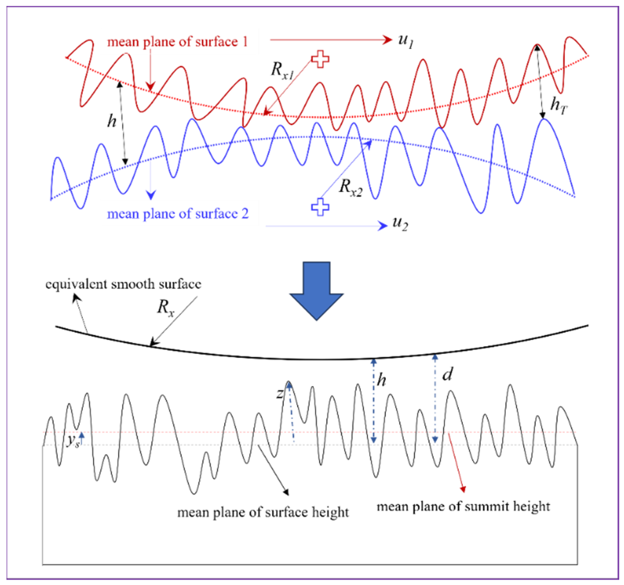
where is the mean rolling speed in the x direction; u1 and u2 are the speeds of surface 1 and surface 2, respectively (see Figure 1); x and y are the axes along and perpendicular to the rolling direction, respectively; is the film fraction related to the cavitation; ph is the hydrodynamic pressure; h is the film thickness; ρ is the density of the lubricant; μ is the zero-shear viscosity of the lubricant; is the ratio of the film thickness (h) to the composite roughness (σ); Ssk is the skewness; Sku is the kurtosis; γ is the pattern ratio; ϕx and ϕy are the pressure flow factors for the Gaussian surface in the x and y directions, respectively, and calculated using Patir and Cheng [13] expressions; and hT is the average gap defined as (Equation (3)) [13]:
where is the Probability Density Function of asperity heights, which is explained later in Section 2.4.1; z = z1 + z2 is the summation of asperity heights, as shown in Figure 1; z1 is the asperity height from the mean plane of surface 1; z2 is the asperity height from the mean plane of surface 2; Rx1 and Rx2 are the radius of curvature of surface 1 and surface 2, respectively; and Rx is the reduced radius of curvature; the symbols ys and d are defined in Section 2.4. According to the Greenwood and Williamson (GW) theory [14], the contact between two rough surfaces can be considered the contact between a smooth, rigid plane and an equivalent (composite) rough surface.
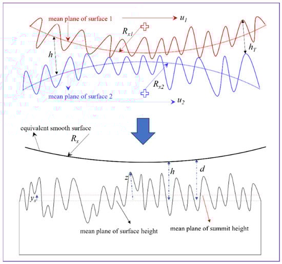
Figure 1.
Schematic of contact between two moving rough surfaces.
2.2. Lubricant Properties
In this work, the lubricant viscosity-pressure relationship was formulated using the Roelands equation (Equation (4)) [18]. Whereas, for the lubricant density–pressure relationship, the expression given by Dowson and Higginson [18] was used (Equation (5)):
where µ0 is the viscosity at ambient conditions; ρ0 is the density at ambient conditions; and ZR is the viscosity–pressure index, which was assumed to 0.68 [28].
2.3. Lubricant Film Thickness
Another important parameter in the lubrication analysis is the film thickness, or the gap height between the mating bodies. The gap height (h) is the function of the rigid body approach (hd), the gap height due to the geometry of contacting surfaces (hg), and the gap height due to elastic deformation of the surfaces (δ). An expression of the gap height (h) is given in Equation (6):
In mixed lubrication, the total pressure generated within the contact zone is supported by both asperity (pa) and hydrodynamic film (ph) pressures and causes an elastic deformation of the mating bodies. The elastic deformation of the surfaces due to ph and pa is given in Equation (7) [9]:
The boundary element method (BEM) was used to discretize the domain area (AH). The fast Fourier transform (FFT) was used to speed-up the computation of the elastic deformation. More information on the calculation of elastic deformation using the fast Fourier transform can be found elsewhere [42].
In mixed lubrication, the external applied load (FN) should be balanced with the total load (Ftot) due to hydrodynamic and asperity pressures. The expression for the load balance is given in Equation (8):
2.4. Asperity Contact Pressure
In this work, the elastic–plastic contact model developed by Zhao et al. [16] was used for the calculation of asperity contact pressure (pa). The expression of asperity pressure, including three stages of asperity deformation (elastic, elastic–plastic, and full plastic), is defined as shown in Equation (9):
where , ; η is the density of summit; β is the mean summit radius; is the distance between the smooth, rigid plane and the mean plane of the summit height; is the distance between the mean plane of the surface and summit height; is the asperity deformation; ; and Hd is the hardness of the material. It should be noted that the starred (*) variables are normalized by σ.
2.4.1. Probability Density Function for the Non-Gaussian Surface
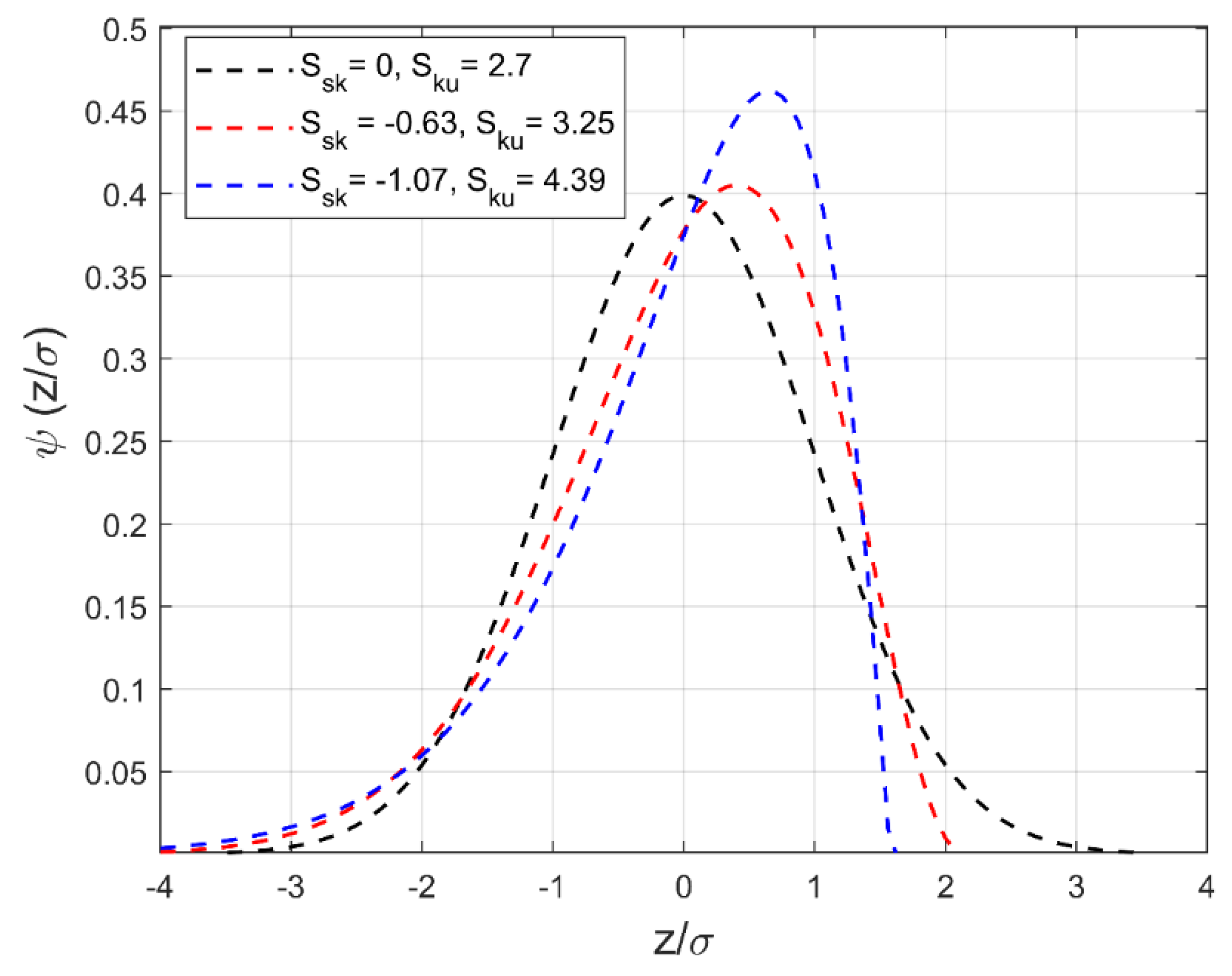
It can be seen from Equations (3) and (9) that the PDF of asperity height is required for the known values of mean, root-mean-square roughness (σ), skewness (Ssk), and kurtosis (Sku) to calculate the average gap height (hT) and asperity contact pressure (pa). In this work, the Pearson system of frequency curves, which is based on the method of moments, was utilized to generate an equation for the different types of PDFs, for which the first four moments (mean, σ, Ssk, and Sku) are known [40]. To use the different PDF equations, a criterion according to Equation (10) was defined by Pearson [40]. By varying the skewness and kurtosis and correspondingly , different types of Pearson curves can be obtained [40]. More information on different types of PDF functions can be found elsewhere [40]. Figure 2 shows the plot of normalized PDFs for different combinations of skewness and kurtosis.
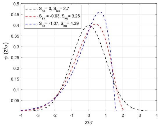
Figure 2.
Normalized probability density functions for normalized asperity heights with different skewness and kurtosis values and a zero mean.
2.5. The Method of Solution
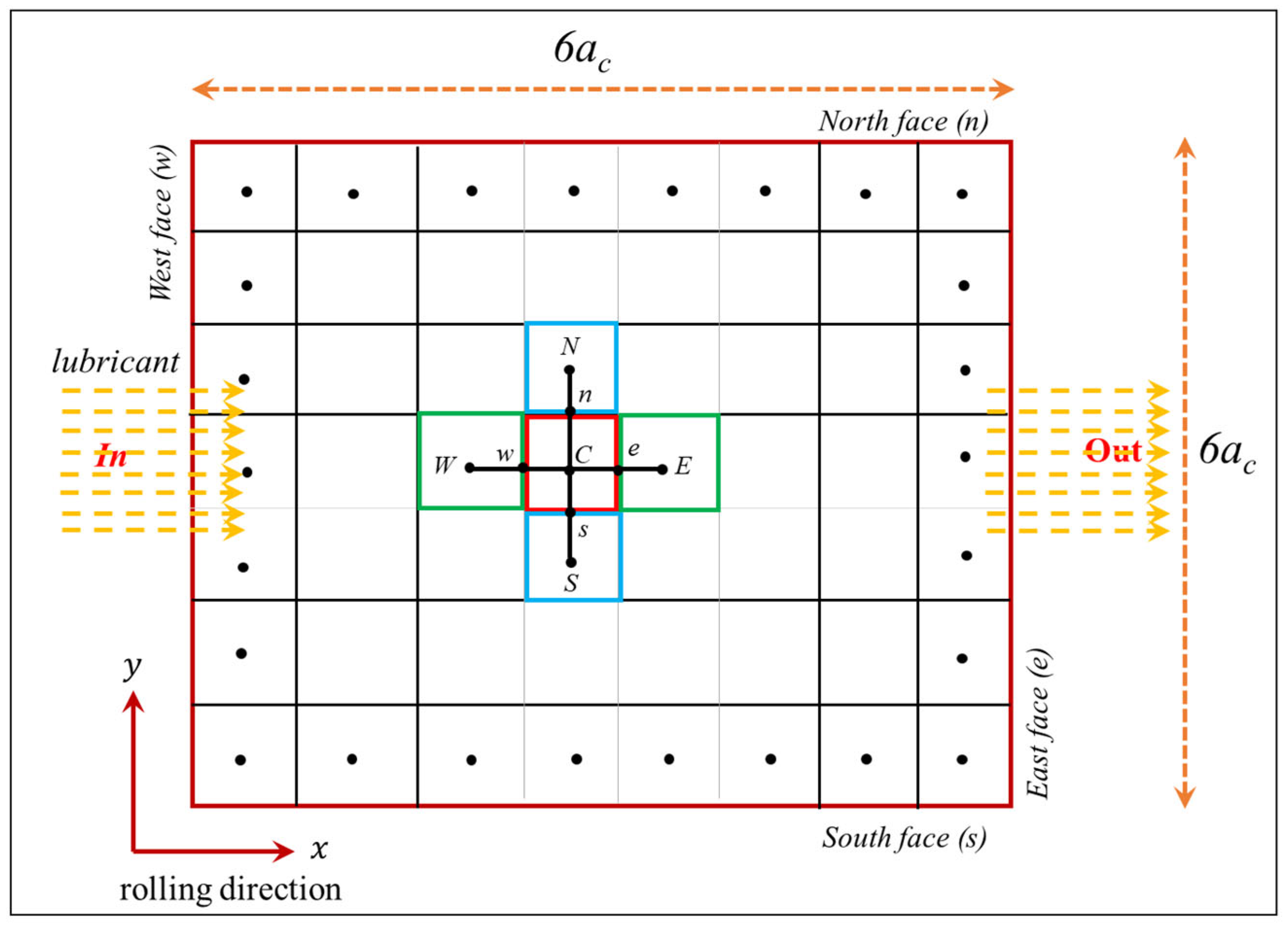
Recently, an extension of the FBNS solver (EHL-FBNS) considering the elastic deformation of contacting bodies has been reported by Hansen et al. [42]. The EHL-FBNS solver, which is based on the Newton–Rapson method, has been proven to be a comparatively fast and efficient solver for EHL analysis [9,18,42]. In this work, the EHL-FBNS algorithm is extended according to Ref. [18] by implementing non-Gaussian flow factors in the Poiseuille terms and the average film thickness in the Couette term of Equation (1). The finite volume method (FVM) was used for discretizing the Poiseuille and Couette terms of Equation (1) [42]. The Poiseuille terms were discretized using a second-order central interpolation scheme, whereas the Couette term was discretized using a first-order upwind interpolation scheme [40]. For the hydrodynamic pressure, the Dirichlet boundary condition (ph = 0) was applied at all faces of the domain [9]. Figure 3 shows a schematic diagram of exemplary stencils within the two-dimensional (2D) discretized EHL domain of size Lx × Ly = 6ac × 6ac (ac is the contact radius), along the east, the west, the north, and the south faces. For cavitation (θ), the Dirichlet boundary condition (θ = 0) was employed on the west face, whereas the Neuman boundary condition was applied to the remaining faces of the domain [9]. To meet the load balance criterion, the rigid body approach (hd) was updated at each iteration using the PID controller method [42] until the load balance tolerance (10−6) was encountered. In this work, the solution was expected to finish when the overall absolute residual () defined by Equation (11) at any iteration number (n) becomes less than or equal to the specified tolerance (1 × 10⁻⁶). The expressions of the residuals used in this work are given in Appendix A. Detailed information on the discretization of the Reynolds equation, the calculation of elastic deformation (δ), and load balance can be found elsewhere [9,42].
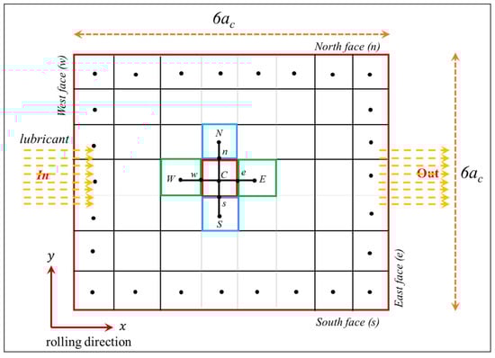
Figure 3.
Schematic sketch of a 2D FVM-based grid with exemplary stencils within the computational domain (E, W, N, and S indicate the centroid of the discretized control volume along the east, west, north, and south faces, respectively).
2.6. Numerical Generation of Artificially Rough Surfaces
It is known that tribological components (i.e., rolling bearings, gears, cams, etc.) are finished by conventional machining processes like grinding, lapping, honing, and shot peening [43]. These machining processes generate various surface features that can be characterized by topography parameters. A brief description of the topography parameters used in Table 1 can be found elsewhere [43]. In this work, a rough surface generation method developed by Pérez-Ràfols et al. [36] was employed. This method uses parameters defining the Weibull height distribution function and power spectral density (PSD) as inputs to generate rough surfaces. Basically, two types of PSD expression (self-affine and exponential) were used. A brief description of the Weibull height distribution function and PSD is given in Appendix B. Table 1 represents the input parameters used for the numerical generation of artificially rough surfaces. The Hurst coefficient (Hf), correlation length (1/λ), and wavelength ratio (Δl/Δs) are related to the spectral properties of the rough surfaces, whereas the shape parameter (kw) is related to the Weibull height distribution function. The Hurst coefficient (Hf) is a parameter that indicates the roughness at the border of the object [44].

Table 1.
Input parameters used for the generation of rough surfaces.
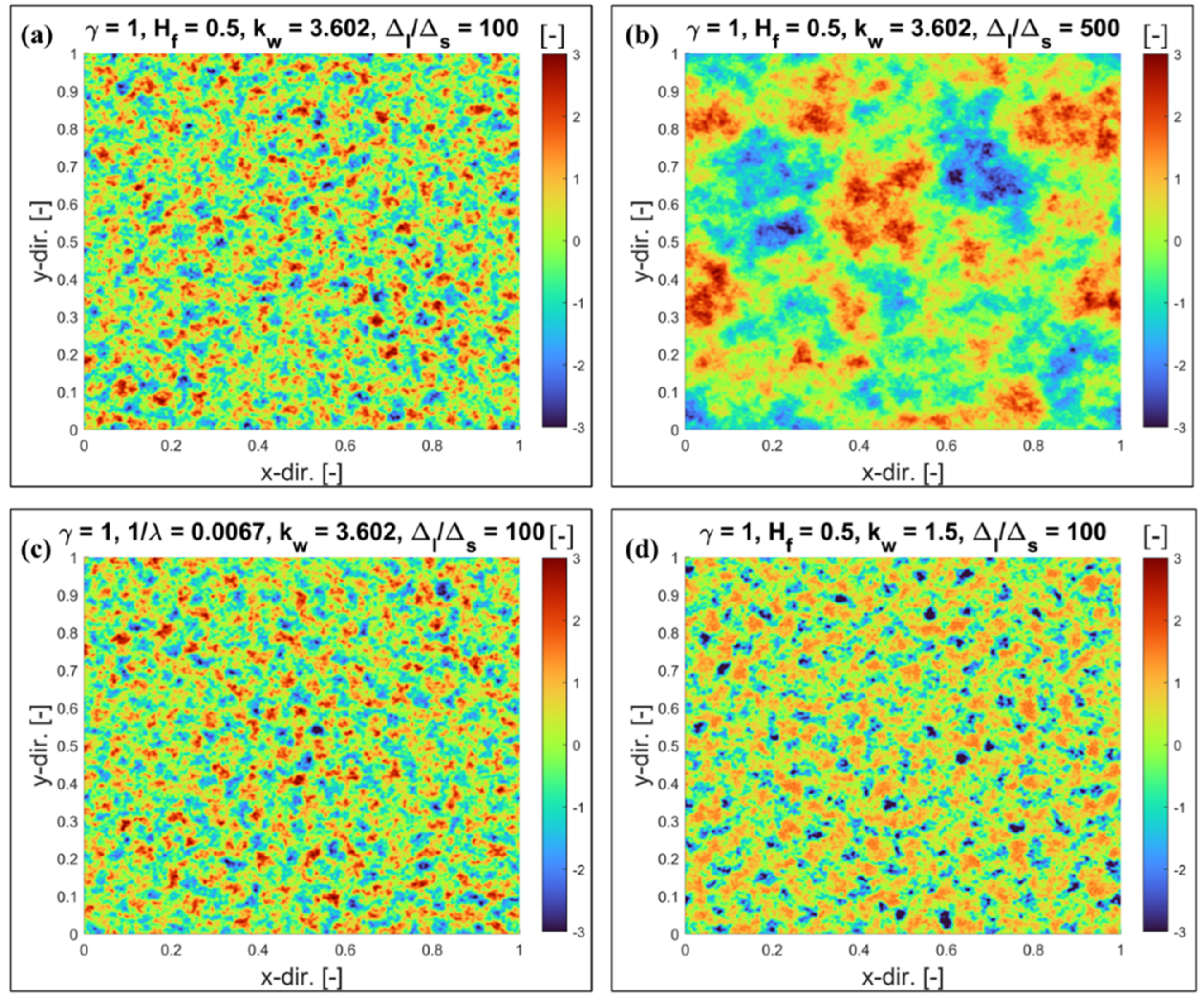
It should be noted that the correlation length (1/λ) was defined whenever an exponential PSD was used as input data for rough surface generation. On the other hand, the Hurst coefficient (Hf) is defined whenever a self-affine PSD is used as input data for rough surface generation. Isometric plots of some of the numerically generated artificial rough surfaces are presented in Figure 4a–d. Each simulated artificial surface consists of 1024 × 1024 data points and a normalized standard deviation, with Sq = 1 [36]. It should be noted that each artificially generated rough surface was scaled to σ = 0.09525 μm before using it as an input in the presented ML model. The sampling interval of 0.1 μm was chosen in the present work to calculate the summit parameters (η and β) by employing the SID (summit identification) method. The summit parameters were used to determine the asperity pressure (pa) (see Equation (9)).
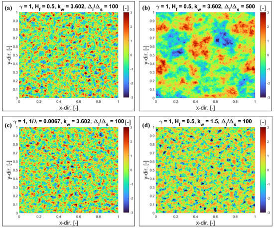
Figure 4.
Isomeric plots of simulated artificial rough surfaces.
3. Results and Discussion
The mixed lubrication model described above is applied to various artificially generated rough surfaces. The influence of various surface features on the asperity load ratio and film parameters is discussed in detail. Several parameters, as presented in Table 2, are multiplied by the corresponding factor to make them dimensionless. From Section 3 and onwards, results are presented in a dimensionless form. Table 3 shows the dimensionless input parameters used throughout the present study. The grid points (257 × 257) and dimensionless domain lengths (−4 to 2 in the X direction and −3 to 3 in the Y direction) are adopted from a recently published work [28]. The Hertzian parameters for the point contact configuration are defined in Appendix C. The asperity load ratio calculated from the present simulation is compared with published results to verify the accuracy of the developed mixed lubrication model.
Table 2.
Parameters and their dimensionless form.
Table 3.
Parameters used in the mixed lubrication simulation.
3.1. The Influence of the Shape Parameter (kw)
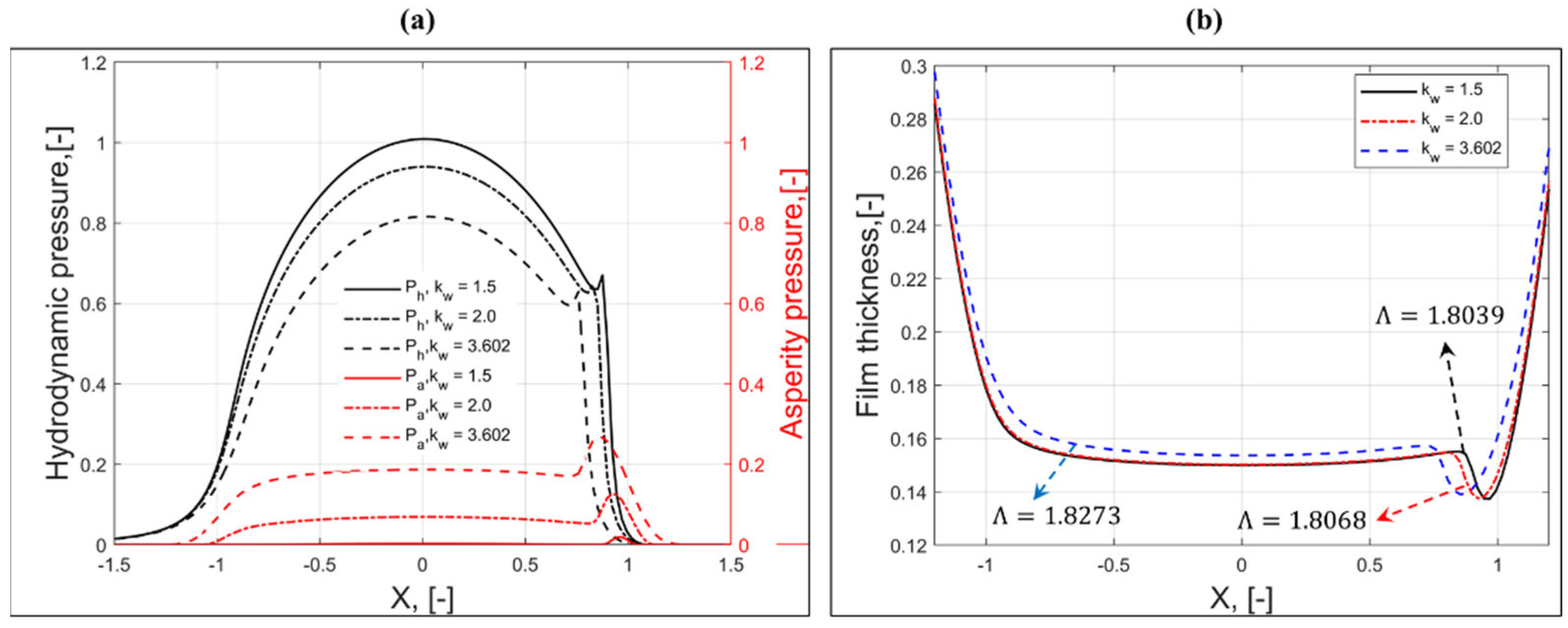
In this section, the effect of the shape parameter (kw) on the asperity load ratio (La) and the film parameter (Λ) is discussed. It has been stated in Refs. [36,45] that lower values of the shape parameter result in higher negative skewness and kurtosis values. For kw = 1.5, Ssk and Sku are −1.07 and 4.39, respectively, and for kw = 2.0, Ssk and Sku are −0.63 and 3.25, respectively [45]. The value of the shape parameter, kw = 3.602, represents the case where asperity heights follow the Gaussian distribution (Ssk = 0, Sku = 2.72) [43]. For kw = 1.5, 2.0, and 3.602, the plot of normalized PDFs is shown in Figure 2 (see Section 2.4.1). The PDFs of rough surfaces for different kw are used to calculate the average film gap (hT) and asperity contact pressure (pa) using Equations (3) and (9), respectively. Figure 5a represents the distribution of dimensionless asperity and hydrodynamic pressures along the X-axis at Y = 0 for different shape parameters. The symbol (-) in the X-axis and Y-axis of Figure 5 indicates that the parameter is presented in dimensionless form. This is also valid for all figures presented in the subsequent sections. As shown in Figure 5a, the dimensionless asperity contact pressure (Pa) increases with an increase in the shape parameter. The rough surfaces with negative skewness exhibit less asperity pressure due to a smaller number of asperity peaks above the mean plane of the surface. For the Gaussian rough surface, high asperity contact pressure is observed due to the significant increase in the number of roughness peaks above the mean plane of the surface. In the middle of the contact zone, the reduction in hydrodynamic pressure is significant and results in an increase in the asperity contact pressure (Pa) due to an increase in the direct asperity-to-asperity contacts. This reduction in hydrodynamic action (EHL lift) due to the change in skewness (Ssk) may affect the fluid frictional force (or coefficient of friction) as well. It can also be observed from Figure 5a that the position of the pressure spike shifts inside the contact zone as kw increases from 1.5 to 3.602. Also, there is a slight reduction in the magnitude of the pressure spike with an increase in the shape parameter. The reduction in the hydrodynamic pressure near the outlet of the contact zone is balanced by the asperity contact pressure, as shown in Figure 5a.
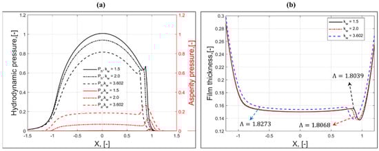
Figure 5.
Distribution of (a) dimensionless hydrodynamic and asperity pressure and (b) dimensionless film thickness along the X-axis and at Y = 0 for different shape parameters (Hf = 0.5, Δl/Δs = 100, and γ = 1).
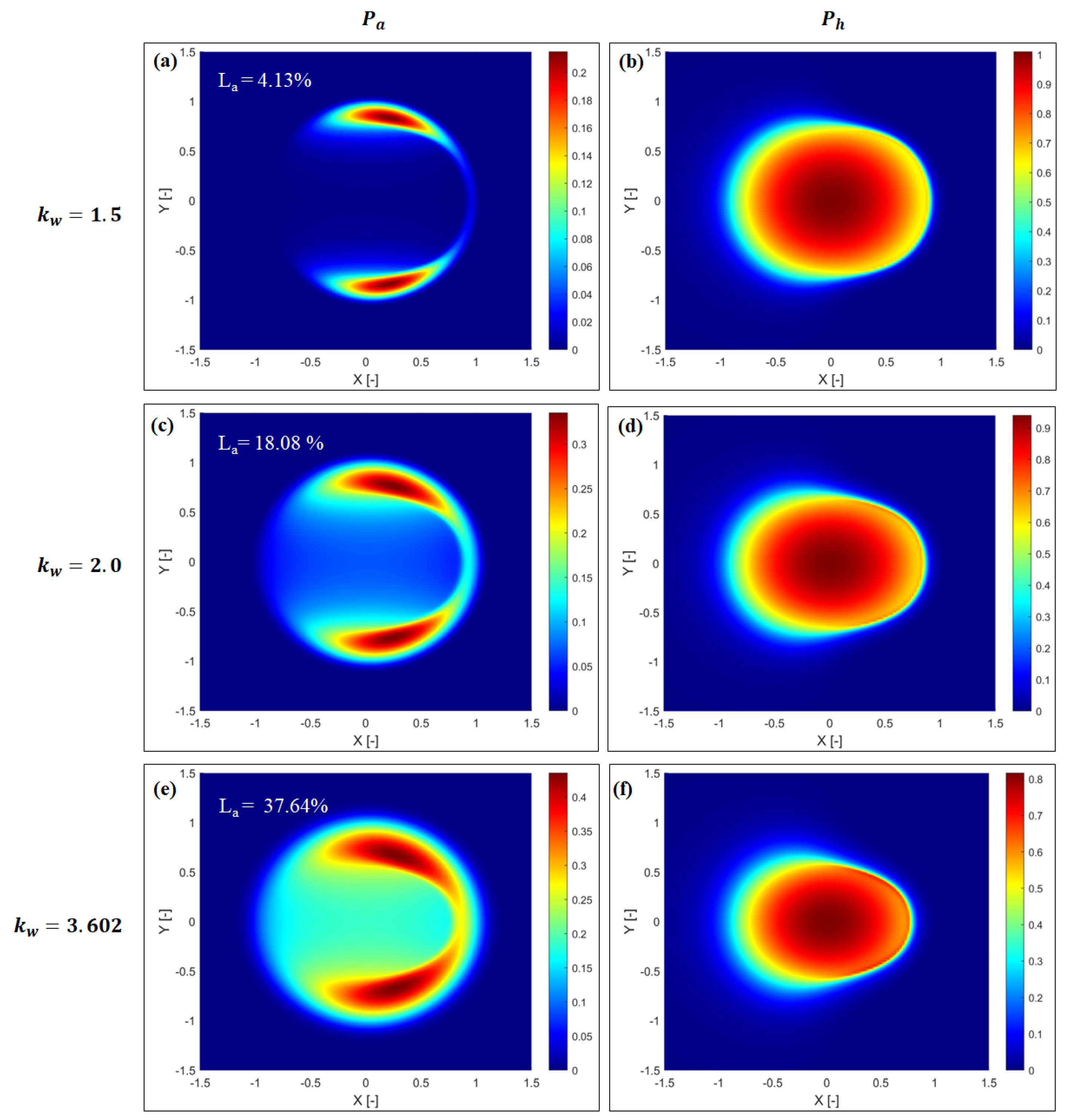
Another interesting observation that can be seen in Figure 5a is that the effect of negative skewness values (for kw = 1.5 and 2) on the Ph is almost negligible near the inlet of the contact zone. However, a decrease in the Ph is found for kw = 3.602 (Gaussian surface). This trend in variation in hydrodynamic pressure near the contact zone inlet should affect the film thickness distribution because the central film thickness is generally affected by a variation in lubricant and surface properties (in the case of ML) at the inlet of the contact zone. Figure 5b shows the distribution of film thickness along the X-axis for different kw. It can be clearly seen from Figure 5b that the film thickness at the inlet as well as at the central part of the contact zone is almost the same for kw = 1.5 and 2.0, which confirms the negligible effect of negative skewness. However, for Gaussian roughness (kw = 3.602), the film thickness increases near the inlet and central part of the contact zone. As illustrated in Figure 5b, the minimum film thickness or film parameter (Λ = hmin/σ) is slightly affected by non-Gaussian roughness. The minimum film thickness, or Λ, increases with an increase in the shape parameter. It can also be observed from Figure 5b that for Gaussian roughness (kw = 3.602), the location of the minimum film thickness is slightly shifted inside of the contact zone due to a significant drop in the hydrodynamic pressure. Isometric plots of dimensionless asperity (Pa) and dimensionless hydrodynamic (Ph) pressure distributions for different shape parameters (kw) are presented in Figure 6a–f. It can be clearly seen that the asperity load ratio (La) increases with an increase in the shape parameter.
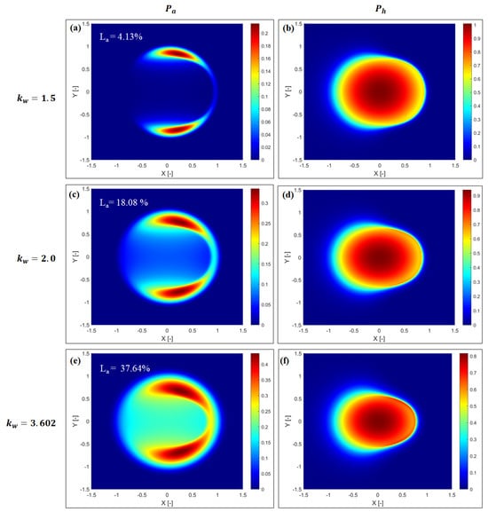
Figure 6.
Isometric plot of (a,b) dimensionless asperity and hydrodynamic pressures for shape parameter (kw) = 1.5; (c,d) dimensionless asperity and hydrodynamic pressures for shape parameter (kw) = 2.0; (e,f) dimensionless asperity and hydrodynamic pressures for shape parameter (kw) = 3.602.
3.2. The Influence of Correlation Length (1/λ)
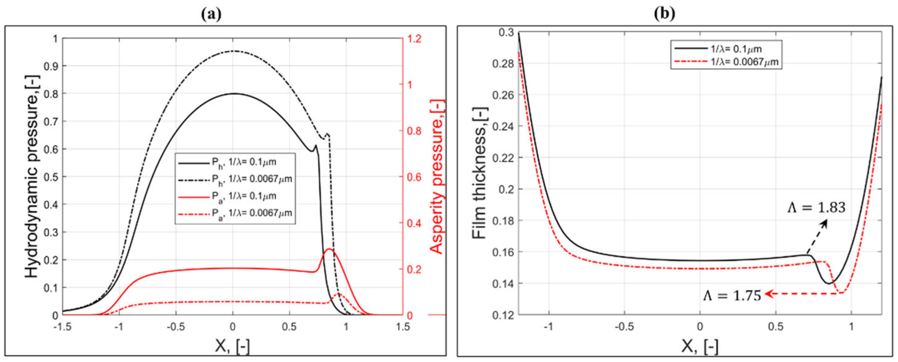
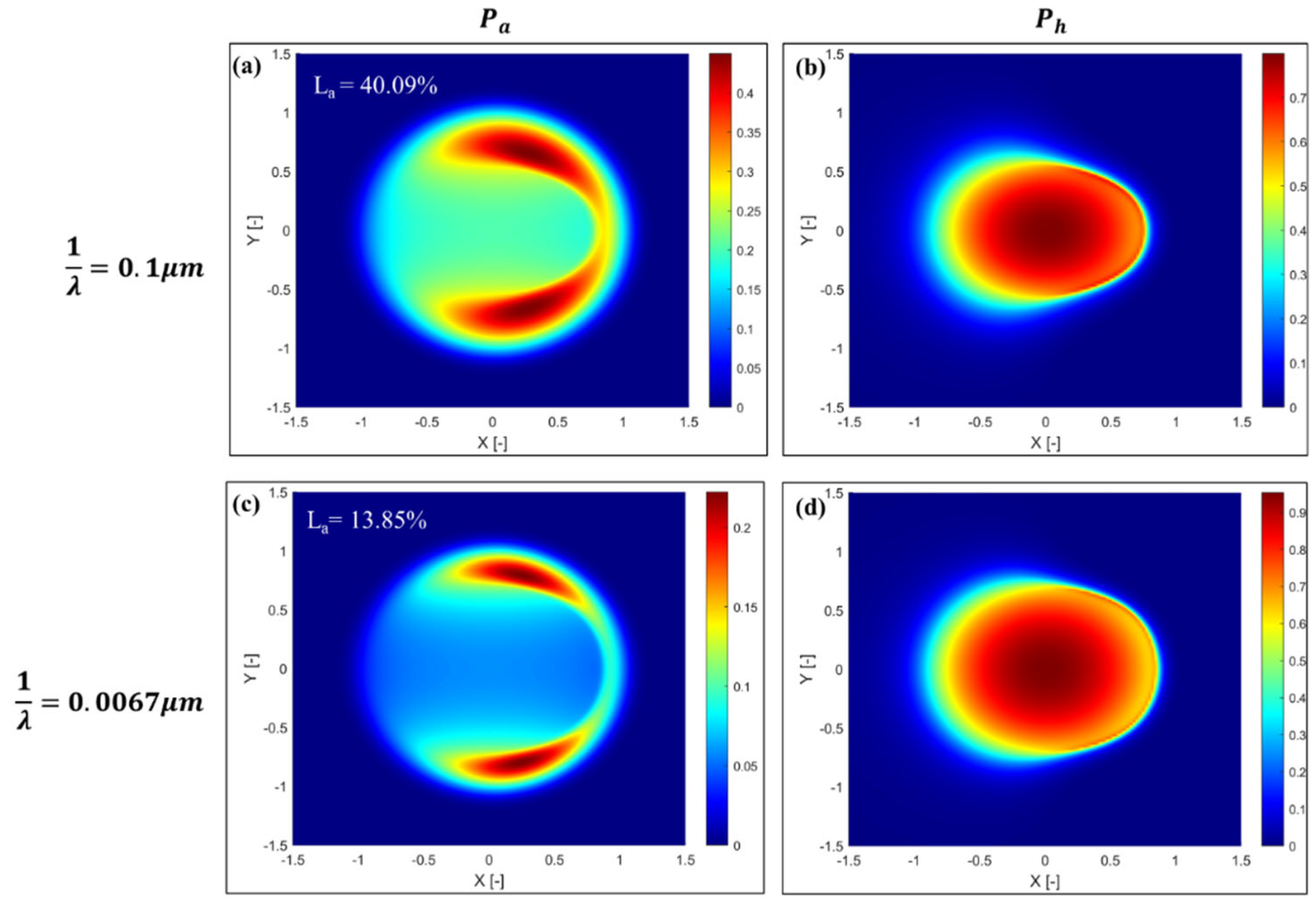
It is known that the correlation length (1/λ) provides the spatial information of rough surfaces [36]. Various engineering rough surfaces display the exponential form of the autocorrelation function () [36], and it has extensively been used for the numerical generation of isotropic rough surfaces [36,45]. The distribution of dimensionless asperity (Pa) and hydrodynamic pressure (Ph) along the X-axis for different correlation lengths is presented in Figure 7a. It can be seen that Ph increases with a decrease in the correlation length (1/λ), and Ph increases significantly for a lower correlation length due to a reduction in asperity-to-asperity contacts (or asperity pressure). A rough surface with a smaller correlation length (1/λ) leads to a smoother surface (flattened roughness peaks), which results in fewer asperity contacts and ultimately leads to a significant reduction in the load carried by asperities. The reduction in Pa at the lower correlation length is shown in Figure 7a. Figure 7b represents the distribution of the dimensionless film thickness along the X-axis for different 1/λ. As illustrated in Figure 7b, the central and minimum film thickness decrease with a decrease in 1/λ. It should, however, be noticed that the location of the occurrence of minimum film thickness slightly increases for lower values of 1/λ due to an increase in the hydrodynamic lift. It can also be seen from Figure 7b that, however, the film parameter (Λ) decreases with a decrease in 1/λ. It can be argued that the film parameter or minimum film thickness should increase for a lower 1/λ due to an increase in the hydrodynamic lift. This happens due to the off-line (macro–micro approach) [46] calculation of asperity contact pressure. This is the prominent reason why full-scale deterministic ML solutions always provide a more feasible film thickness, or Λ [46]. Figure 8a–d represent isometric plots of Pa and Ph for different correlation lengths (1/λ). It can be clearly seen that the asperity load ratio (La) decreases with a decrease in the correlation length (1/λ).
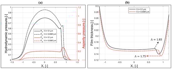
Figure 7.
Distribution of (a) dimensionless hydrodynamic and asperity pressure and (b) dimensionless film thickness along the X-axis and at Y = 0 for different correlation lengths (Δl/Δs = 100, γ = 1, and kw = 3.602).
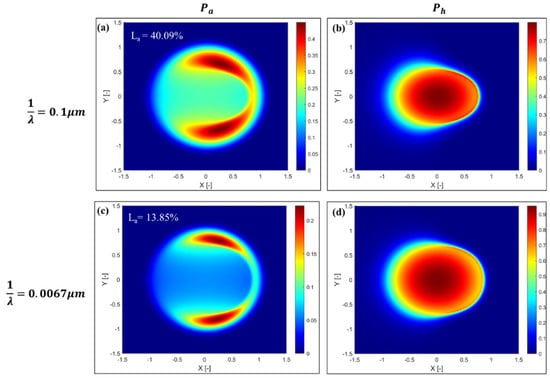
Figure 8.
Isometric plots of (a,b) dimensionless asperity and hydrodynamic pressures for correlation length (1/λ) = 0.1 μm; (c,d) dimensionless asperity and hydrodynamic pressures for correlation length (1/λ) = 0.0067 μm.
3.3. The Influence of the Wavelength Ratio (Δl/Δs)
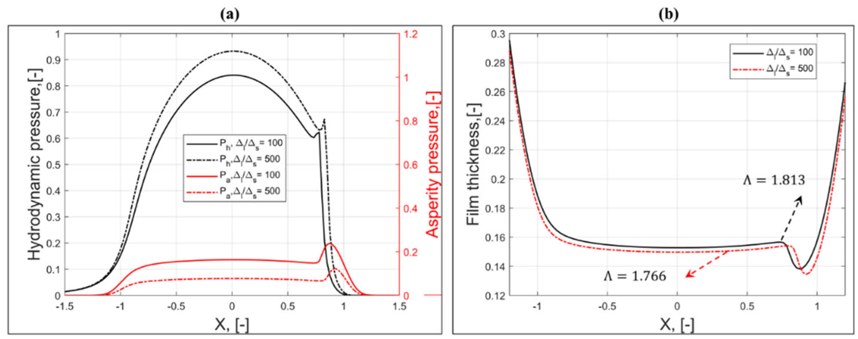
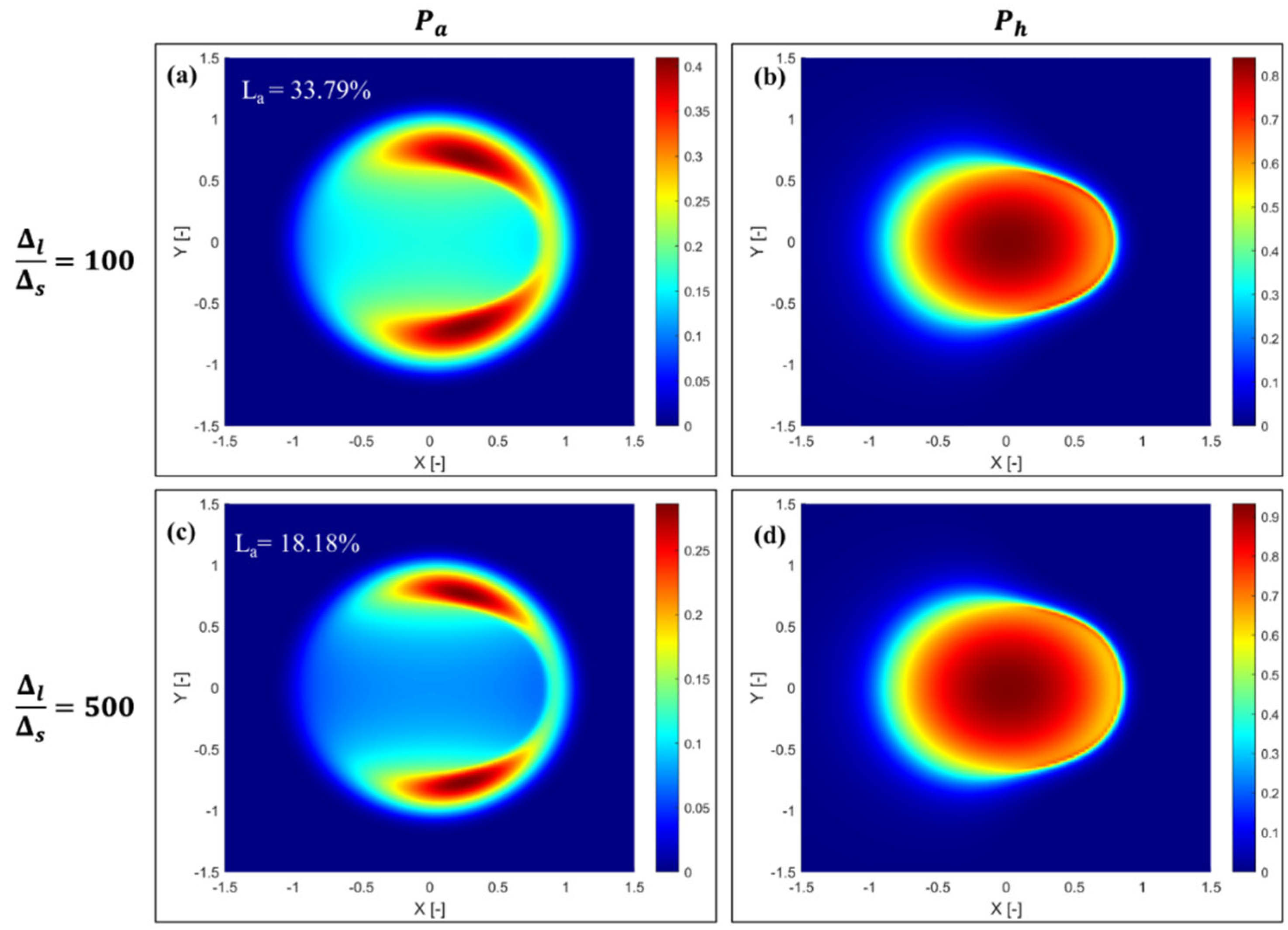
As stated in Refs. [36,45], the wavelength ratio (Δl/Δs) is related to lower and upper cut-off frequencies (ql and qs), which have been used to define the width of the power spectrum of a rough surface. It has been suggested in Ref. [36] that the wavelength ratio should not be less than 100 to generate a Gaussian rough surface with sufficient accuracy in the HPD (height probability distribution). In this work, two different values of wavelength ratio (Δl/Δs = 100 and 500) are chosen, and its effect on mixed lubrication is investigated. Figure 9a represents the variation of dimensionless asperity and hydrodynamic pressure along the X-axis for different Δl/Δs. It can be seen that the Ph increases with an increase in Δl/Δs. For Δl/Δs = 500, a significant increase in Ph is observed in the middle of the contact zone, whereas a small increment in Ph is observed near the inlet and outlet of the contact zone. Also, the location of the pressure spike is shifted towards the inside of the contact zone for lower Δl/Δs. Higher values of the Δl/Δs ratio eliminate the high frequency components, and the simulated rough surface contains mostly high wavelength components, which ultimately leads to flattened roughness peaks (see Figure 4b). The flattened roughness peaks at higher Δl/Δs ratios result in fewer asperity-to-asperity contacts, which ultimately diminishes the asperity pressure. As a result, an increase in hydrodynamic lift occurs for high Δl/Δs ratios. The film thickness distribution along the rolling direction for different Δl/Δs ratios is presented in Figure 9b. It can be seen that the central and minimum film thickness (or film parameter) decrease with an increase in the Δl/Δs ratio. Figure 10a–d represent the isometric plot of asperity and hydrodynamic pressures for different Δl/Δs ratios. It can be clearly seen that the asperity load ratio (La) significantly decreases with an increase in the Δl/Δs ratio.
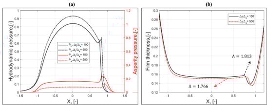
Figure 9.
Distribution of (a) dimensionless hydrodynamic and asperity pressure and (b) dimensionless film thickness along the X-axis and at Y = 0 for different wavelength ratios (Hf = 0.5, γ = 1, and kw = 3.602).
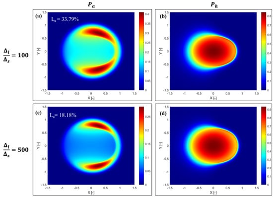
Figure 10.
Isometric plot of (a,b) dimensionless asperity and hydrodynamic pressures for wavelength ratio (Δl/Δs) = 100; (c,d) dimensionless asperity and hydrodynamic pressures for wavelength ratio (Δl/Δs) = 500.
3.4. The Influence of the Hurst Coefficient (Hf)
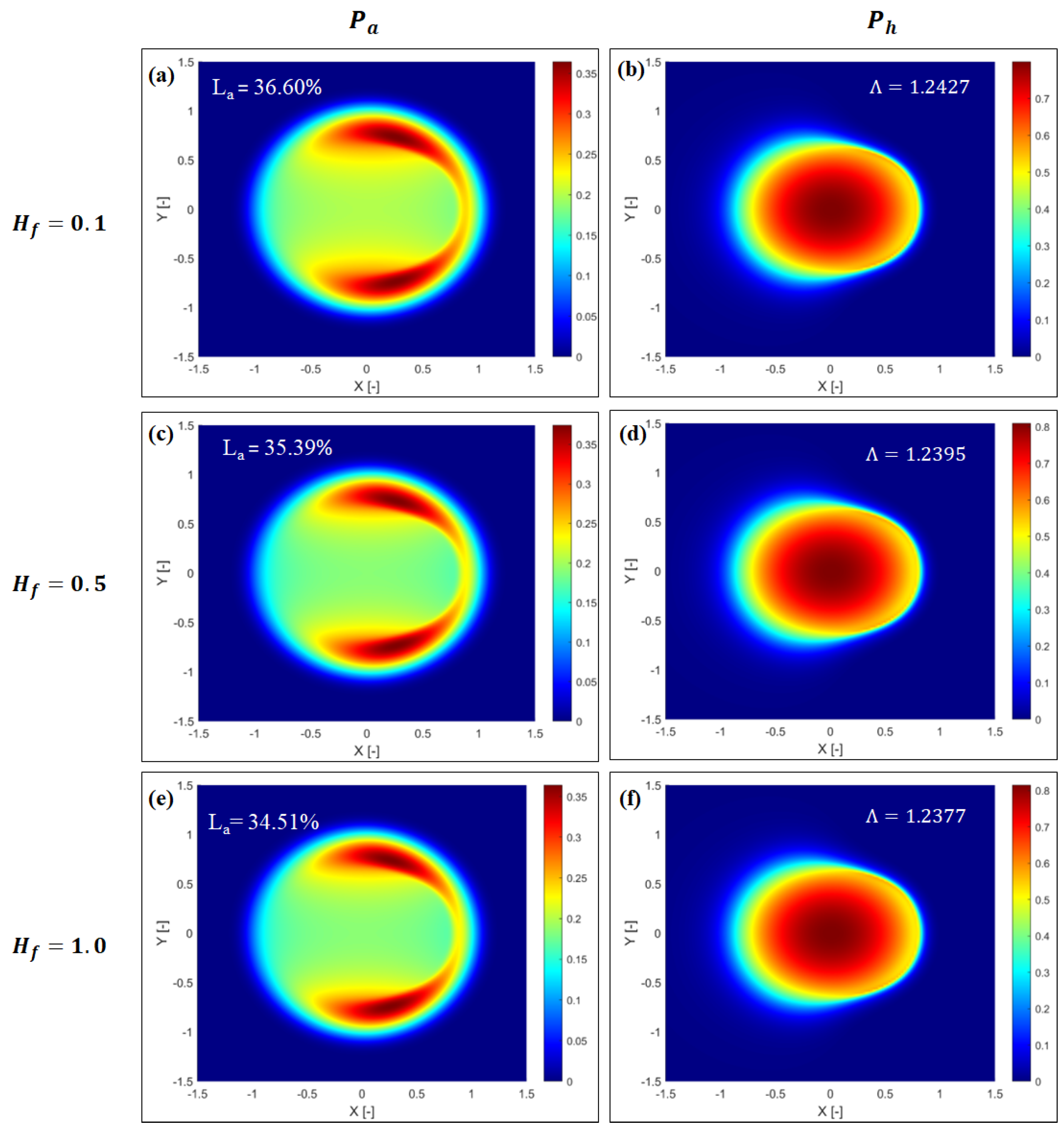
Recently, it has been reported by Prajapati and Tiwari [44] that theoretically, the root-mean-square (RMS) roughness (σ) and RMS slope () decrease with an increase in Hurst coefficient. The theoretical trend between σ and Hf has also been confirmed by performing pin-on-disc pure sliding experiments [44]. Figure 11a shows the variation of dimensionless asperity and hydrodynamic pressures along the X-axis for different Hf. It can be seen that Pa decreases with an increase in Hf. As illustrated in Figure 11a, the change in Pa and Ph is quite distinct at the midpoint of the contact zone. The reason for a slight decrease in Pa at higher Hf is due to the smoothness of the simulated surface, which increases with an increase in Hf. A smoothed rough surface consists of blunt roughness peaks, which results in fewer asperity contacts and ultimately decreases the asperity pressure. It can also be seen from Figure 11a that the change in Pa and Ph with Hf is almost negligible near the inlet and outlet of the contact zone, which indicates a small change in minimum film thickness. The film thickness plot for different Hf values is shown in Figure 11b. As postulated, Figure 11b confirms the small variation of the central and minimum film thickness with Hf. Isometric plots of Pa and Ph for different Hf are presented in Figure 12a–f. It can clearly be seen from Figure 12 that the asperity load ratio (La) decreases with an increase in Hf. A slight decrease in the film parameter (Λ) at higher Hf is also observed in Figure 12b,d,f.
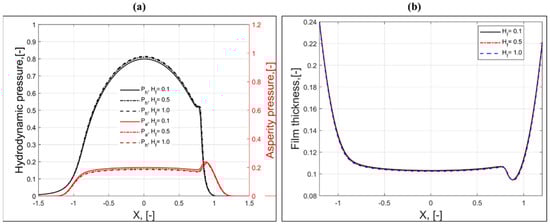
Figure 11.
Distribution of (a) dimensionless hydrodynamic and asperity pressure and (b) dimensionless film thickness along the X-axis and at Y = 0 for different Hurst coefficients (Δl/Δs =100, γ = 1, and kw = 3.602).
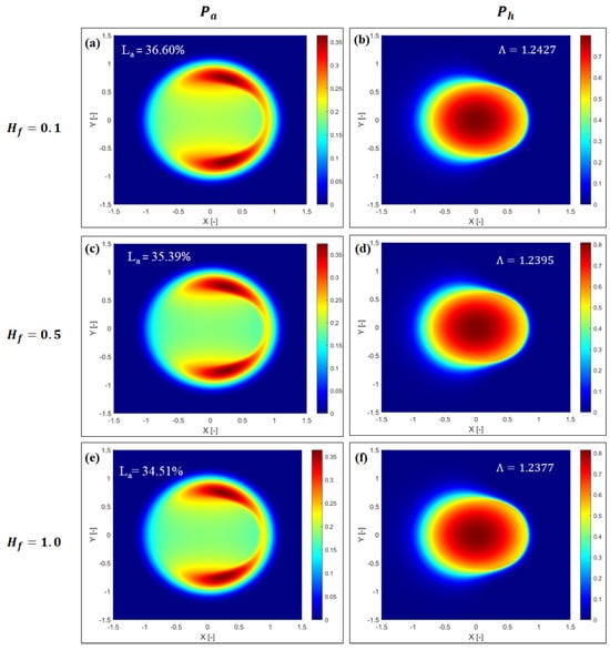
Figure 12.
Isometric plots of (a,b) dimensionless asperity and hydrodynamic pressures for Hurst coefficient (Hf) = 0.1; (c,d) dimensionless asperity and hydrodynamic pressures for Hurst coefficient (Hf) = 0.5; (e,f) dimensionless asperity and hydrodynamic pressures for Hurst coefficient (Hf) = 1.
3.5. Validation of the Model
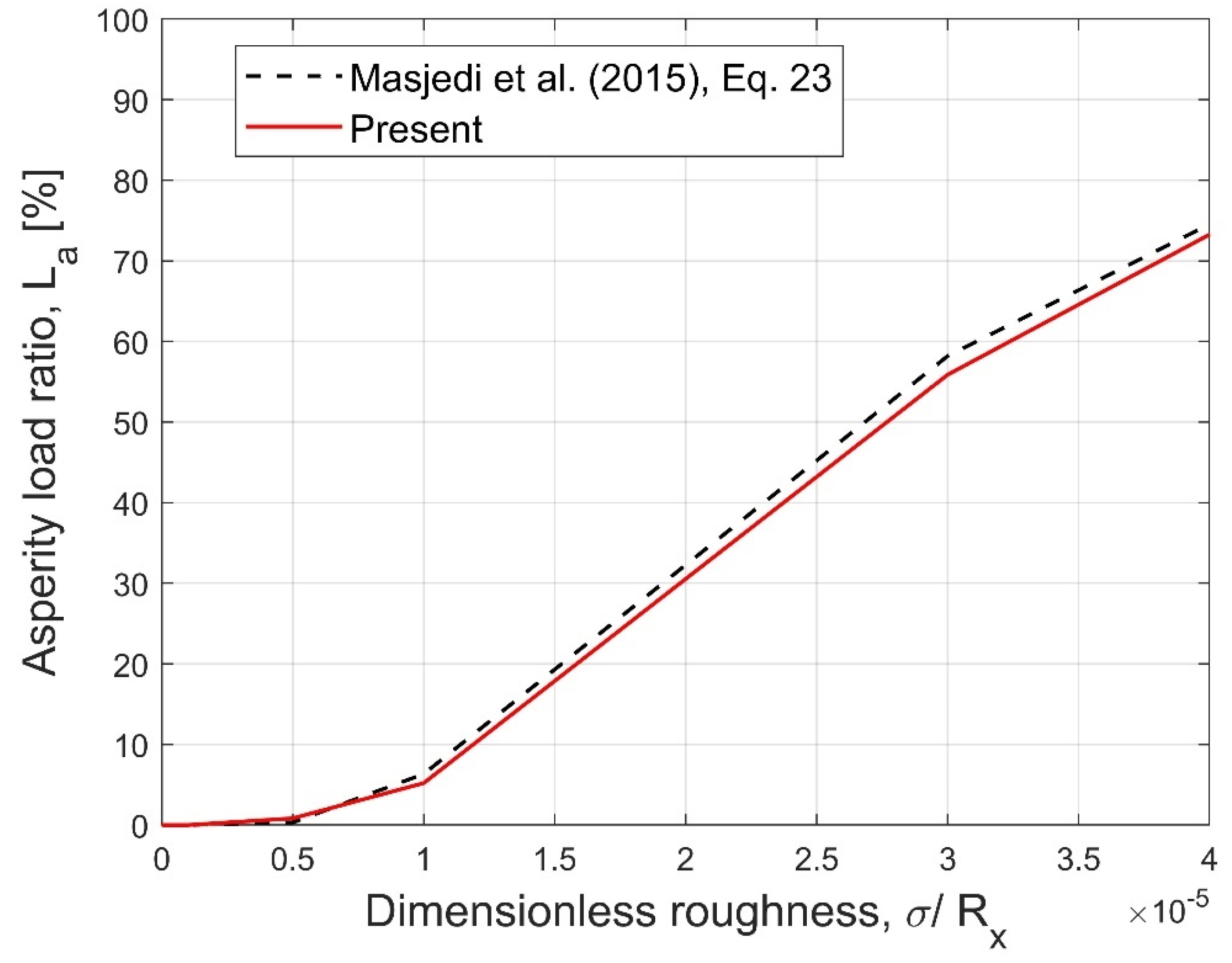
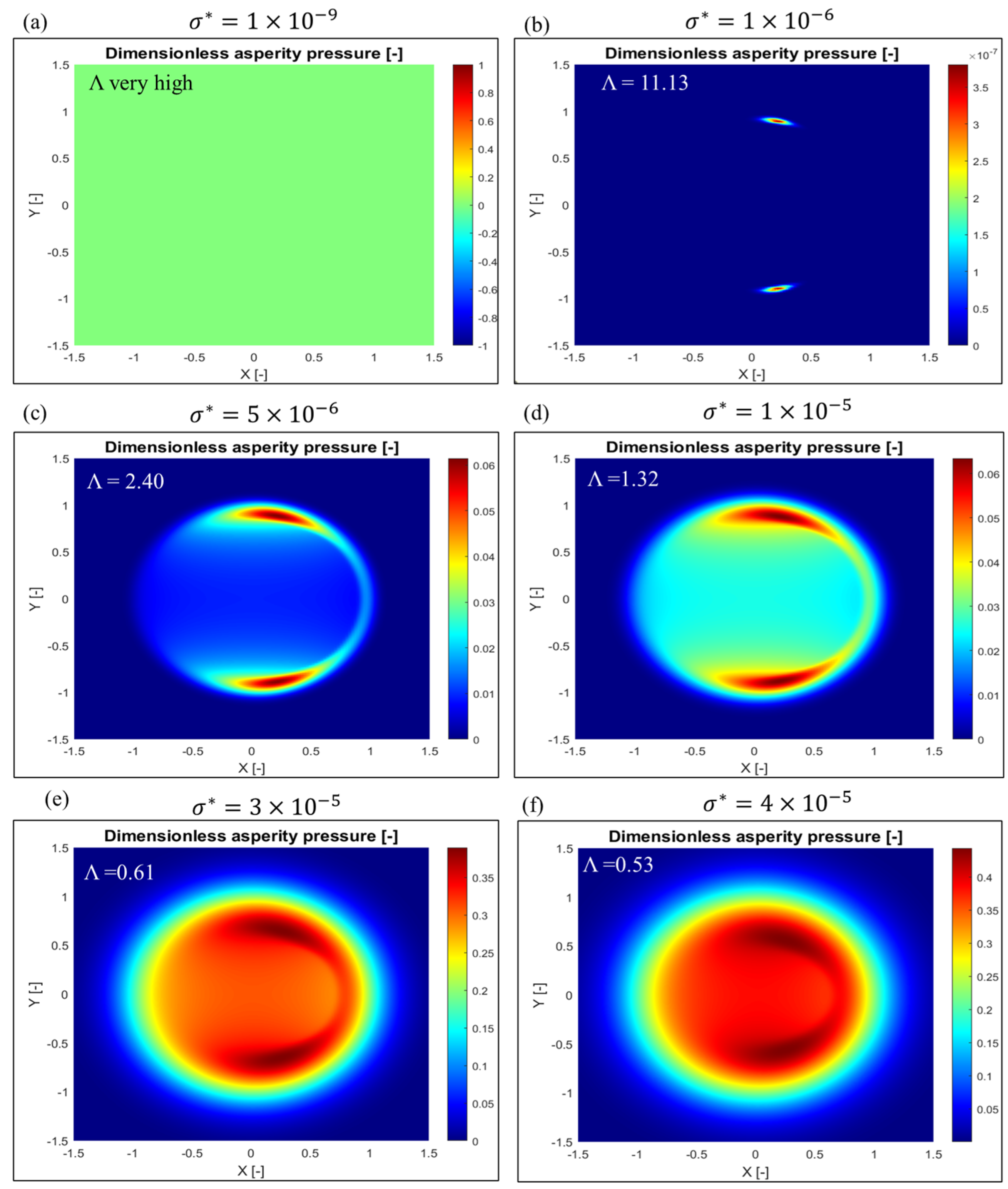
To date, an expression for determining asperity load ratio (La) and film thickness (central and minimum) for non-Gaussian roughness has not been developed. However, Masjedi and Khonsari [20] developed an expression for calculating the asperity load ratio for the Gaussian roughness (Ssk = 0 and Sku = 3). Therefore, the asperity load ratio calculated by the present method and the Masjedi and Khonsari [20] La expression are compared. For model validation only, the following input parameters are used in the ML simulation: W = 1 × 10⁻⁶, U =1 × 10⁻¹¹, G = 4972, V = 0.01, ηβσ = 0.05, and β/σ = 100 [20]. As illustrated in Figure 13, the overall trend is relatively reliable. It can also be seen from Figure 13 that the La obtained by the present method is slightly smaller than the Masjedi and Khonsari [20] La expression. This can be attributed to the enormous differences between EHL solvers and convergence criteria. Figure 14a–f represent isometric plots of dimensionless asperity pressure (using the present method) for different dimensionless roughness (σ*). The film parameter (Λ) is also indicated in Figure 14a–f. It can be observed that for very low roughness (), the asperity pressure is completely zero in the EHL domain. The asperity pressure increases inside the contact zone with an increase in dimensionless roughness (σ*). As shown in Figure 14, the film parameter (Λ) is very high for the smooth surface and decreases with an increase in dimensionless roughness levels (σ*). It can be inferred from Figure 14 that the present ML model excellently simulates the mixed lubrication and full film regimes.
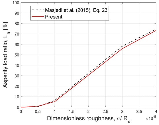
Figure 13.
Comparison of asperity load ratio (La) obtained by Masjedi and Khonsari [20] La expression and present method.
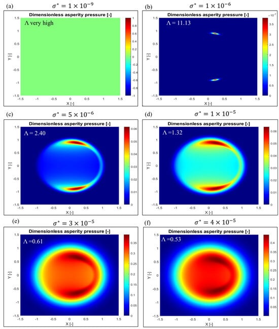
Figure 14.
Isometric plots of dimensionless asperity pressure (present method) for different dimensionless roughness levels (σ* = σ/Rx).
4. Conclusions
In this work, the impact of non-Gaussianity on the mixed lubrication parameters (film parameter and asperity load ratio) is addressed. Non-Gaussian artificial rough surfaces are generated by specifying the Weibull height distribution function and power spectral density (PSD). This allows studying the mixed lubrication in a parametric way while ensuring that the studied artificially rough surfaces have practical significance. Using a non-Gaussian topography generation algorithm and a mixed lubrication modeling framework, a parametrized study is conducted, considering the shape parameter kw, the correlation length 1/λ, the Hurst coefficient Hf, and the wavelength ratio (Δl/Δs). The main findings from the present work can be summarized as follows:
- For the specified operating conditions (W = 1 × 10⁻⁶, U = 1 × 10⁻¹¹, G = 4972, V = 0.03, and σ* = 1 × 10⁻⁵), it is found that the film parameter (Λ) varies between one and three for each artificial rough surface, which ensures the manifestation of the mixed lubrication regime. It is also shown that the present ML model excellently simulates the mixed and full-film lubrication regimes.
- It is revealed that the shape parameter (kw) leads to a significant change in the asperity height distribution. A change in the asperity height distribution profoundly affects the asperity and hydrodynamic pressures. It is found that the asperity load ratio increases from 4% to 38% as the shape parameter increases from 1.5 (non-Gaussian) to 3.602 (Gaussian). A slight increase in the film parameter is observed as the asperity height distribution changes from non-Gaussian to Gaussian.
- It is concluded that a higher wavelength ratio increases the hydrodynamic lift significantly. The asperity load ratio decreases with an increase in wavelength ratio. The film parameter slightly decreases at higher wavelength ratios.
- It is observed that the Hurst coefficient (Hf) slightly improves the hydrodynamic action. At the middle of the contact zone, a small increase in the hydrodynamic lift is observed for a large value of the Hurst coefficient (Hf > 0.1). A trivial effect of the Hurst coefficient is found on the film thickness or film parameter. It is also found that the hydrodynamic lift increases with a decrease in the correlation length (1/λ) due to a significant drop in the asperity load ratio (La).
- The present ML model is validated from Ref. [20], and a good match is found by comparing the asperity load ratio (La) for different dimensionless surface roughness levels (σ*).
Furthermore, it will be interesting to develop the formulas for determining the film thickness (central and minimum) and asperity load ratio by considering the non-Gaussian roughness, roughness orientations, and spectral properties of rough surfaces. Also, the present analysis can be extended to study the effects of contact angles on the lubrication performance of heavily loaded counterformal contacts.
Author Contributions
Conceptualization: D.K.P.; Methodology: D.K.P. and M.B.; Data curation: D.K.P.; Analysis of data: D.K.P. and M.B.; Writing- draft preparation: D.K.P.; Review and editing: D.K.P. and M.B.; Supervision: M.B. All authors have read and agreed to the published version of the manuscript.
Funding
This research was funded by the Kempe Foundation, grant number SMK-2043.
Data Availability Statement
The original contributions presented in the study are included in the article. Any further inquiries can be communicated to the corresponding author.
Acknowledgments
The authors sincerely acknowledge the Fractal Surface Generator (version 1.1.0) which is an MATLAB-based open source software and was accessed on 10 December 2023
Conflicts of Interest
The authors declare no conflicts of interest.
Nomenclature
| 1/λ | Correlation length, m |
| Ah | EHL domain area, m2 |
| β | Mean summit radius, m |
| Δl | Shortest cut-off wavelength |
| Δs | Longest cut-off wavelength |
| η | Summit density, m−2 |
| G | Dimensionless material parameter |
| γ | Anisotropy factor |
| h | Film thickness, m |
| Hc | Dimensionless central film thickness |
| hd | Rigid body approach, m |
| Hf | Hurst coefficient |
| hmin | Minimum film thickness, m |
| Hmin | Dimensionless minimum film thickness |
| hT | Average gap height, m |
| La | Asperity load ratio, % |
| ML | Mixed lubrication |
| pa | Dimensional hydrodynamic pressure, Pa |
| Pa | Dimensionless asperity pressure |
| ph | Dimensional hydrodynamic pressure, Pa |
| Ph | Dimensionless hydrodynamic pressure |
| R(r) | Autocorrelation function for isotropic surface |
| Rx | Reduced radius of curvature, mm |
| σ | Composite root-mean-square (RMS) roughness, m |
| SRR | Slide-to-roll ratio, ur/um |
| Ssk | Skewness |
| Sku | Kurtosis |
| ur | Sliding speed, (u2−u1), m/s |
| um | Mean rolling speed, (u1 + u2/2), m/s |
| U | Dimensionless speed parameter |
| W | Dimensionless load parameter |
| x | Dimensional X-axis, m |
| X | Dimensionless X-axis |
| y | Dimensional Y-axis, m |
| Y | Dimensionless Y-axis |
Appendix A. Expression of Residuals
In this work, different residuals are used to check load convergence, asperity pressure convergence, hydrodynamic pressure convergence, and cavitation convergence. The expressions for calculating these residuals are given in Equations (A1)–(A4) [9,40]:
where n is the iteration number; FN is the total applied normal load; is the incremental asperity pressure at the nth iteration; is the incremental hydrodynamic pressure at the nth iteration; is the incremental cavitation fraction at the nth iteration; is the total load due to asperity and hydrodynamic pressure at the nth iteration; and is the incremental cavitation fraction at the nth iteration.
Appendix B. A Brief Description of Weibull Height Distribution and PSD
Appendix B.1. Probability Density Function for Weibull Distribution of Asperity Heights
An expression for the dimensionless Weibull distribution is given in Equation (A5) [36]. It can be seen that it is a two-parameter distribution function. In Equation (A5), kw is called the shape parameter, and α is known as the scale parameter. The scale parameter is calculated using Equation (A6) [36]:
where is the gamma function, and z* is the asperity height normalized by σ.
Appendix B.2. Power Spectral Density (PSD)
In this work, self-affine and exponential forms of power spectral density were used for rough surface generation. The expressions for self-affine and exponential PSD are given in Equations (A7) and (A8), respectively [36]:
where ql and qs are the lower and upper frequency cut-offs, respectively; qx and qy are the wave numbers of the spectral content in the X and Y directions, respectively; is the power spectral density; 1/λ is the correlation length; C0 is the scale constant; and Δl/Δs= qs/ql,
.
Appendix C. Hertzian Point Contact
Using the Hertzian point contact theory, analytical expressions for determining the contact parameters for point contact configuration are given in Equations (A9)–(A11):
where ac is the contact radius; E1 and E2 are the elastic moduli of body 1 and body 2, respectively; ν1 and ν2 are the Poisson ratios of body 1 and body 2, respectively; Eeq is the equivalent elastic modulus; Rx is the reduced radius of curvature; pmax is the maximum Hertzian pressure; and FN is the total applied normal load.
References
- Spikes, H.A.; Olver, A.V. Basics of Mixed Lubrication. Lub. Sci. 2003, 16, 128. [Google Scholar] [CrossRef]
- Maier, M.; Pusterhofer, M.; Summer, F.; Grun, F. Validation of Statistic and Deterministic Asperity Contact Models Using Experimental Stribeck Data. Trib. Int. 2022, 165, 107329. [Google Scholar] [CrossRef]
- Hansen, J.; Bjorling, M.; Larsson, R. A New Film Parameter for Rough Surface EHL Contacts with Anisotropic and Isotropic Structures. Tribol. Lett. 2021, 69, 37. [Google Scholar] [CrossRef]
- He, T.; Zhu, D.; Wang, J.; Wang, Q.C. Experimental and Numerical Investigations of the Stribeck Curves for Lubricated Counterformal Contacts. ASME J. Tribol. 2017, 139, 021505. [Google Scholar] [CrossRef]
- Xu, G.; Sadeghi, F. Thermal EHL Analysis of Circular Contacts with Measured Surface Roughness. ASME J. Tribol. 1996, 118, 473–483. [Google Scholar] [CrossRef]
- Zhu, D.; Ai, X. Point Contact EHL Based on Optically Measured Three-Dimensional Rough Surfaces. ASME J. Tribol. 1997, 119, 375–384. [Google Scholar] [CrossRef]
- Hu, Y.Z.; Zhu, D. A Full Numerical Solution to the Mixed Lubrication in Point Contacts. ASME J. Tribol. 2000, 122, 1–9. [Google Scholar] [CrossRef]
- Patir, N.; Cheng, H. Application of Average Flow Model to Lubrication between Rough Sliding Surfaces. J. Tribol. 1979, 101, 220–229. [Google Scholar] [CrossRef]
- Hansen, E.; Vaitkunaite, G.; Schneider, J.; Gumbsch, P.; Frohnapfel, B. Establishment and Calibration of a Digital Twin to Replicate the Friction Behaviour of a Pin-on-Disk Tribometer. Lubricants 2023, 11, 75. [Google Scholar] [CrossRef]
- Zhang, S.; Zhang, C. A New Deterministic Model for Mixed Lubricated Point Contact with High Accuracy. ASME J. Tribol. 2021, 143, 102201. [Google Scholar] [CrossRef]
- Wang, Y.; Dorgham, A.; Liu, Y.; Wang, C.; Wilson, M.C.T.; Neville, A.; Azam, A. An Assessment of Quantitative Predictions of Deterministic Mixed Lubrication Solvers. ASME J. Tribol. 2020, 143, 011601. [Google Scholar] [CrossRef]
- Zhu, D.; Cheng, H.S. Effect of Surface Roughness on the Point Contact EHL. ASME J. Tribol. 1988, 110, 32–37. [Google Scholar] [CrossRef]
- Patir, N.; Cheng, H. An Average Flow Model for Determining Effects of Three-Dimensional Roughness on Partial Hydrodynamic Lubrication. J. Tribol. 1978, 100, 12–17. [Google Scholar] [CrossRef]
- Greenwood, J.A.; Williamson, J.B.P. Contact of Nominally Flat Surfaces. Proc. R. Soc. A Math. Phys. Eng. Sci. 1966, 295, 300–319. [Google Scholar]
- Greenwood, J.A.; Tripp, J.H. The Contact of Two Nominally Flat Rough Surfaces. Proc. Inst. Mech. Eng. 1970, 185, 625–633. [Google Scholar] [CrossRef]
- Zhao, Y.; Maietta, D.M.; Chang, L. An Asperity Microcontact Model Incorporating the Transition from Elastic Deformation to Fully Plastic Flow. J. Tribol. 2001, 122, 86–93. [Google Scholar] [CrossRef]
- Kogut, L.; Etsion, I. A Finite Element-Based Elastic-Plastic Model for the Contact of Rough Surfaces. Tribol. Trans. 2003, 46, 383–390. [Google Scholar] [CrossRef]
- Gu, C.; Zhang, D.; Jiang, X.; Meng, X.; Wang, S.; Ju, P.; Liu, J. Mixed EHL Problems: An Efficient Solution to the Fluid–Solid Coupling Problem with Consideration of Elastic Deformation and Cavitation. Lubricants 2022, 10, 311. [Google Scholar] [CrossRef]
- Prajapati, D.K. Numerical Analysis of Rough Hydrodynamic Bearings for Various Deterministic Micro-Asperity Features. Surf. Topogr. Metrol. Prop. 2021, 9, 015004. [Google Scholar] [CrossRef]
- Masjedi, M.; Khonsari, M.M. On the Effect of Surface Roughness in Point-Contact EHL: Formulas for Film Thickness and Asperity Load. Tribol Int. 2015, 82, 228–244. [Google Scholar] [CrossRef]
- Masjedi, M.; Khonsari, M.M. Film Thickness and Asperity Load Formulas for Line-Contact Elastohydrodynamic Lubrication with Provision for Surface Roughness. ASME J. Tribol. 2012, 134, 011503. [Google Scholar] [CrossRef]
- Masjedi, M.; Khonsari, M.M. Mixed Elastohydrodynamic Lubrication Line-Contact Formulas with Different Surface Patterns. Proc. Inst. Mech. Eng. Part J J. Eng. Tribol. 2014, 228, 849–859. [Google Scholar] [CrossRef]
- Moraru, L.; Keith, T.G., Jr. Application of the Amplitude Reduction Technique within Probabilistic Rough EHL Models. ASME J. Tribol. 2009, 131, 021703. [Google Scholar] [CrossRef]
- Wu, C.; Qu, P.; Zhang, L.; Li, S.; Jiang, Z. A numerical and experimental study on the interface friction of ball-on-disc test under high temperature. Wear 2017, 376–377, 433–442. [Google Scholar] [CrossRef]
- Zhang, H.; Dong, G.; Dong, G. A Mixed Elastohydrodynamic Lubrication Model Based on Virtual Rough Surface for Studying the Tribological Effect of Asperities. Ind. Lubr. Tribol. 2018, 70, 408–417. [Google Scholar] [CrossRef]
- Leighton, M.; Rahmani, R.; Rahnejat, H. Surface-Specific Flow Factors for Prediction of Friction of Cross-Hatched Surfaces. Surf. Topogr. Metrol. Prop. 2016, 4, 025002. [Google Scholar] [CrossRef]
- Pei, J.; Han, X.; Tao, Y.; Feng, S. Mixed Elastohydrodynamic Lubrication Analysis of Line Contact with Non-Gaussian Surface Roughness. Tribol. Int. 2020, 151, 106449. [Google Scholar] [CrossRef]
- Hou, H.; Pei, J.; Cao, D.; Wang, L. Study on Mixed Elastohydrodynamic Lubrication Performance of Point Contact with Non-Gaussian Rough Surface. Lubr. Sci. 2023, 36, 51–64. [Google Scholar] [CrossRef]
- Morales-Espejel, G.E. Flow Factors for Non-Gaussian Roughness in Hydrodynamic Lubrication: An Analytical Interpolation. Proc. Inst. Mech. Eng. Part C J. Mech. Eng. Sci. 2009, 223, 1433–1441. [Google Scholar] [CrossRef]
- Kim, T.; Cho, Y. The Flow Factors Considering the Elastic Deformation for the Rough Surface with A Non-Gaussian Height Distribution. Tribol. Trans 2008, 51, 213–220. [Google Scholar] [CrossRef]
- Meng, F.; Qin, D.; Chen, H.; Hu, Y.; Wang, H. Study on Combined Influence of Inter-Asperity Cavitation and Elastic Deformation of Non-Gaussian Surfaces on Flow Factors. Proc. Inst. Mech. Eng. Part C J. Mech. Eng. Sci. 2008, 222, 1039–1048. [Google Scholar] [CrossRef]
- Zhang, Y.; Kovalev, A.; Hayashi, N.; Nishiura, K.; Meng, Y. Numerical Prediction of Surface Wear and Roughness Parameters during Running-in for Line Contacts under Mixed-Lubrication. ASME J. Tribol. 2018, 140, 061501. [Google Scholar] [CrossRef]
- Gu, C.; Meng, X.; Wang, S.; Ding, X. Research on Mixed Lubrication Problems of the Non-Gaussian Rough Textured Surface with Influence of Stochastic Roughness in Consideration. ASME J. Tribol. 2019, 141, 12501. [Google Scholar] [CrossRef]
- Prajapati, D.K.; Ramkumar, P.; Katiyar, J.K. Research on Tribological Performance of Piston Ring/Liner Conjunction Considering Non-Gaussian Roughness and Cavitation. Proc. Inst. Mech. Eng. Part C J. Eng. Tribol. 2023, 237, 732–745. [Google Scholar] [CrossRef]
- Prajapati, D.K.; Katiyar, J.K.; Prakash, C. Determination of Friction Coefficient for Water Lubricated Journal Bearing Considering Rough EHL Contacts. Int. J. Interact. Des. Manuf. 2023. [Google Scholar] [CrossRef]
- Pérez-Ràfols, F.; Almqvist, A. Generating Randomly Rough Surfaces with Given Height Probability Distribution and Power Spectrum. Tribol. Int. 2019, 131, 591–604. [Google Scholar] [CrossRef]
- Prajapati, D.K.; Ahmed, D.; Katiyar, J.K.; Prakash, C.; Ajaj, R.M. A Numerical Study on the Impact of Lubricant Rheology and Surface Topography on Heavily Loaded Non-Conformal Contacts. Surf. Topogr. Metrol. Prop. 2023, 11, 035006. [Google Scholar] [CrossRef]
- Lubrecht, A.A.; Venner, C.H. Elastohydrodynamic lubrication of rough surfaces. Proc. Inst. Mech. Eng. Part C J. Eng. Tribol. 1999, 213, 397–404. [Google Scholar] [CrossRef]
- Sperka, P.; Krupka, I.; Hart, M. Experimental study of real roughness attenuation in concentrated contacts. Tribol. Int. 2010, 43, 1893–1901. [Google Scholar] [CrossRef]
- Kotwal, C.A.; Bhushan, B. Contact Analysis of Non-Gaussian Surfaces for Minimum Static and Kinetic Friction and Wear. Tribol Trans. 1996, 39, 890–898. [Google Scholar] [CrossRef]
- Woloszynski, T.; Podsiadlo, P.; Stachowiak, G.W. Efficient Solution to the Cavitation Problem in Hydrodynamic Lubrication. Tribol. Lett. 2015, 58, 18. [Google Scholar] [CrossRef]
- Hansen, E.; Kacan, A.; Frohnapfel, B.; Codrignani, A. An EHL Extension of the Unsteady FBNS Algorithm. Tribol. Lett. 2022, 70, 80. [Google Scholar] [CrossRef]
- Prajapati, D.K.; Tiwari, M. Assessment of Topography Parameters during Running-in and Subsequent Rolling Contact Fatigue Tests. ASME J. Tribol. 2019, 141, 051401. [Google Scholar] [CrossRef]
- Prajapati, D.K.; Tiwari, M. The Relation between Fractal Signature and Topography Parameters: A Numerical and Experimental Study. Surf. Topogr. Metrol. Prop. 2018, 6, 045008. [Google Scholar] [CrossRef]
- Sabino, T.S.; Carneiro, A.M.C.; Carvalho, R.P.; Pires, F.M.A. Evolution of the Real Contact Area of Self-Affine Non-Gaussian Surfaces. Int. J. Solids Struct. 2023, 268, 112173. [Google Scholar] [CrossRef]
- Wang, Q.J.; Zhu, D.; Cheng, H.S.; Yu, T.; Jiang, X.; Liu, S. Mixed Lubrication Analyses by a Macro-Micro Approach and Full-Scale Mixed EHL Model. ASME J. Tribol. 2004, 126, 81–91. [Google Scholar] [CrossRef]

Disclaimer/Publisher’s Note: The statements, opinions and data contained in all publications are solely those of the individual author(s) and contributor(s) and not of MDPI and/or the editor(s). MDPI and/or the editor(s) disclaim responsibility for any injury to people or property resulting from any ideas, methods, instructions or products referred to in the content. |
© 2024 by the authors. Licensee MDPI, Basel, Switzerland. This article is an open access article distributed under the terms and conditions of the Creative Commons Attribution (CC BY) license (https://creativecommons.org/licenses/by/4.0/).