Digital Twin-Driven Thermal Error Prediction for CNC Machine Tool Spindle

Abstract

Traditional methods for predicting thermal error ignore the correlation between physical world data and virtual world data, leading to the low prediction accuracy of thermal errors and affecting the normal processing of the CNC machine tool (CNCMT) spindle. To solve the above problem, we propose a thermal error prediction approach based on digital twins and long short-term memory (DT-LSTM). DT-LSTM combines the high simulation capabilities of DT and the strong data processing capabilities of LSTM. Firstly, we develop a DT system for the thermal characteristics analysis of a spindle. When the DT system is implemented, we can obtain the theoretical value of thermal error. Then, the experimental data is used to train LSTM. The output of LSTM is the actual value of thermal error. Finally, the particle swarm optimization (PSO) algorithm fuses the theoretical values of DT with the actual values of LSTM. The case study demonstrates that DT-LSTM has a higher accuracy than the single method by nearly 11%, which improves the prediction performance and robustness of thermal error.

1. Introduction

The performance of CNCMT is largely measured by its machining precision. Error is an important factor that influences machining precision. Generally, the error of CNCMT has a geometric error, thermal error, and force-induced error. Thermal error accounts for the highest proportion [1]. According to the existing literature, the thermal error is the major manufacturing error of CNCMT. With the improvement of the manufacturing level, the geometric accuracy of CNCMT has improved, and geometric errors have gradually decreased. The impact of thermal error on processing and manufacturing has become increasingly prominent. Therefore, exploring the thermal error of the CNCMT spindle system is a hot topic.

The spindle system is the main subsystem of CNCMT. The quick prediction and accurate compensation of thermal error can enhance the machining precision of CNCMT. Currently, there are two methods for constructing a thermal error model for CNCMT. One is the LSTM-based thermal error model. The other is the DT-based thermal error model [2]. However, the large heat sources and rapid speed changes of the CNCMT spindle system lead to significant time-varying thermal errors [3]. Based on a single thermal error modeling method, it is difficult to achieve a real-time and accurate reflection of the physical spindle system, which seriously hinders the efficient operation of CNCMT.

We propose a hybrid thermal error prediction method based on DT and LSTM. DT-LSTM improves the real-time reflection, accuracy, and robustness of thermal error prediction for the CNCMT spindle system. The rest of the paper is organized as follows. Section 2 introduces the related works of thermal error prediction. Section 3 presents the implementation of DT-LSTM. Section 4 shows a case study on how to predict thermal error based on DT-LSTM. Finally, conclusions are drawn in Section 5.

2. Related Works

2.1. LSTM-based Thermal Error Prediction

Zimmermann et al. designed a new self-adaptive approach for thermal error prediction [4]. Liang et al. developed an LSTM-based thermal error prediction model for heavy-duty CNCMT [5]. Li et al. reviewed LSTM thermal error modeling methods for MTs [6]. Li et al. proposed a thermal error prediction approach for electrical spindles using an optimized extreme learning machine algorithm [7]. Liao et al. established a robust thermal error model for spindles based on the improved fruit fly optimization algorithm [8]. Kumar et al. designed a real-time LSTM-based predictive model for thermal perception [9]. Li et al. established a multiple regression approach, which used nut temperature and ambient temperature as independent variables of the model [10]. Abdulshahed et al. considered the impact of nut temperature and bearing temperature on a thermal error and established a thermal error approach using gray neural networks [11]. Zhu et al. added additional temperature key points to prediction models (e.g., multiple regression models and neural network models), which enhanced the prediction accuracy of the approach [12]. Yang et al. established a finite element approach to the thermal error and the nut temperature rise, which predicted the spindle thermal error [13].

An LSTM-based model with high prediction performance is established when it obtains sufficient input and output data. If the data is not comprehensive enough, the established approach will be difficult to adapt to various situations. The poor robustness is characteristic of LSTM-based modeling. To obtain excellent robustness, the LSTM-based error prediction approach should combine with the DT system.

2.2. DT-based Thermal Error Modeling

Some scholars designed a DT system to predict thermal error. Liu et al. presented a DT system of thermal error prediction for gear profile grinders [14]. Ma et al. presented a self-learning-empowered thermal error prediction approach for machine tools based on DT [15]. Xiao et al. developed a DT system to analyze the thermal characteristics of the MT spindle [16]. Liu et al. designed an error prediction model for the MT spindle using DT [17]. To enhance the prediction performance of thermal error, Yi et al. designed a DT-based system [18]. Liu et al. designed a comprehensive machining thermal error approach based on DT [19]. Lunev et al. assessed the thermal performance of metal foams based on DT [20]. Kuprat et al. presented a thermal characterization analysis approach using DT for a power semiconductor [21].

The DT model based on hypothetical operating conditions is inconsistent with the actual operating conditions of the equipment, which leads to inconsistent models and low prediction accuracy. Therefore, we use data-based models to correct DT simulation data. It enhances the prediction performance of thermal errors and the processing precision of CNCMT.

3. DT-LSTM

3.1. DT

DT creates virtual models of real objects. DT combines models, data, and integration technologies. It achieves the coverage of the entire product lifecycle process and the connectivity and interaction between physical space and information space [22]. Grieves first proposed the concept of DT and defined the 3D model of DT (e.g., physical product, virtual product, and connection) [23]. NASA has successfully applied DT to aircraft health management. Tao et al. introduced DT into the field of intelligent manufacturing and presented the concept of DT workshop [24], which promoted the research and development of DT. The evolution characteristics of the spindle DT system are complex, dynamic, and stochastic. Therefore, we detect and correct the thermal boundary of physical equipment and map it to virtual entities. The actual thermal characteristic of physical equipment is obtained via finite element simulation, which improves the accuracy of the thermal characteristic.

3.2. LSTM

LSTM is a time cycle network. When there is a time series relationship between the processed task and time, LSTM has excellent processing and prediction performance. The spindle thermal deformation has a time series characteristic. Therefore, LSTM can predict spindle thermal error.

LSTM has the forget gate, input gate, and output gate [25]. At the previous time, the preservation degree of the unit state is determined by the forget gate. At the current time, the preservation degree of the unit state is determined by the input gate. The output gate determines the output degree of the unit state to the current output value. Figure 1 shows the network structure of LSTM.

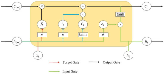
Figure 1. The architecture of LSTM.

The forget gate is given by [26] as follows:

$$f_t=\sigma \left(W_f\cdot \left[h_{t-1},x_t\right]+b_f\right),$$

(1)

where $f_t$ denotes the forget information; $\sigma$ denotes the sigmoid function; $W_f$ represents the weight coefficient; $h_{t-1}$ represents the last moment output; $x_t$ represents the input at the time t; $b_f$ represents the offset.

The input gate formulate is given by [26] as follows:

$$i_t=\sigma \left(W_i\cdot \left[h_{t-1},x_t\right]+b_i\right),$$

(2)

$$\tilde{C}=\tanh \left(W_c\cdot \left[h_{t-1},x_t\right]+b_C\right),$$

(3)

where $i_t$ and ${\tilde{C}}_t$ denote the input information; $\tanh$ denotes the tanh function; $W_i$ and $W_C$ represent the weight coefficient; $b_i$ and $b_C$ represent the offset.

The updated cell information is given by [26] as follows:

$$C_t=f_t\cdot C_{t-1}+i_t\cdot {\tilde{C}}_t,$$

(4)

where $C_{t-1}$ is the old cell information.

The output formula of LSTM is given by [26] as follows:

$$o_t=\sigma \left(W_o\cdot \left[h_{t-1},x_t\right]+b_o\right),$$

(5)

$$h_t=o_t\cdot \tanh \left(C_t\right),$$

(6)

where $W_o$ denotes the weight coefficient; $b_o$ denotes the offset; $h_t$ denotes the current moment output.

3.3. DT-LSTM

3.3.1. Framework

Figure 2 shows the framework of DT-LSTM. DT-LSTM combines LSTM and DT to obtain high prediction accuracy. Based on material characteristics and operating conditions, a multi-domain DT model for the CNCMT spindle is established. The temperature field is simulated using the working condition mapping of the CNCMT spindle. The internal temperature state of the CNCMT spindle is calculated as a virtual sensing signal. Meanwhile, the thermal error prediction approach using LSTM is performed on the actual signal. Finally, the PSO algorithm is applied to combine theoretical value and actual value. The LSTM observation result modifies the DT simulation result.

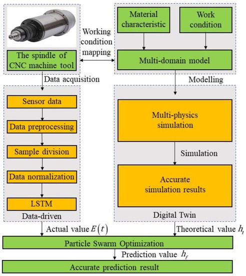
Figure 2. The framework of DT-LSTM.

3.3.2. Implementation

(1)

The implementation of the DT model

DT model implementation is shown in Figure 3. During DT model building, multi-domain knowledge (e.g., thermal boundary condition, thermal deformation field, and thermal characteristic theory) must be considered simultaneously. Multi-domain modeling software contains ANSYS and UG. Therefore, object models from the spindle system can be constructed and embedded into a unified multi-domain model.

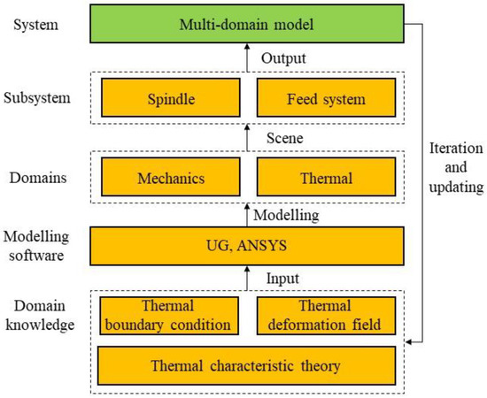
Figure 3. The implementation of the DT model.

• Thermal boundary condition

a.

Bearing heat calculation

The main heat source of the CNCMT spindle system is the bearing, and the friction torque of the bearing generates the heat. The generated heat is given by [27] as follows:

$$Q_1=1.047\times {10}^{-4}nM,$$

(7)

where $Q_1$ represents the generated heat of bearing; $n$ represents the speed of bearing; $M$ represents the friction torque of bearing.

$M$ is equal to the sum of the load-unrelated friction torque $M_0$ and the load-related friction torque $M_1$.

$$M=M_0+M_1,$$

(8)

$$M_0={10}^{-7}{f}_0{\left(v_{0}n\right)}^{2/3}{D}_m^3{M}_0·v_{0}n\ge 2000,$$

(9)

$$M_0=160f_0{D}_m^3·v_{0}n<2000,$$

(10)

where $f_0$ represents the friction constant; $v_0$ represents the kinematic viscosity; $D_m$ represents the average diameter of bearing [27].

$$M_1=0.0013f_1{(X_0{F}_r+Y_0{F}_a/C_0)}^{10/3}{D}_m,$$

(11)

where $f_1$ represents the load constant; $C_0$ represents the basic load rating; $X_0$ represents the distribution coefficient of the radial load; $Y_0$ represents the distribution coefficient of the axial load; $F_r$ represents the radial load; $F_a$ represents the axial load [27].

b.

Screw-nut heat calculation

The heating principle of the lead screw-nut is identical to the bearing. The calculation formula is given by [27] as follows:

$$Q_2=0.12\pi n\prime M\prime ,$$

(12)

where $Q_2$ represents the generated heat of the lead screw-nut; $n\prime$ represents the speed of the lead screw-nut; $M\prime$ represents the friction torque of the lead screw-nut.

The calculation formula of $M\prime$ is given by [27] as follows:

$$M\prime =2z\left(M_e+M_g\right)\cos \beta ,$$

(13)

where $z$ is the ball number; $\beta$ is the helical angle of the lead screw spiral raceway; $M_e$ is the friction resistance torque; $M_g$ is the geometric sliding friction torque.

The calculation formula of $z$ is given by [27] as follows:

$$z=i\left(\frac{\pi d}{d_0}-3\right),$$

(14)

where $i$ represents the coefficient; $d_0$ represents the ball diameter; $d$ represents the nominal diameter of the lead screw.

The calculation formula of $M_e$ and $M_g$ are given by [27] as follows:

$$M_e=m_{\beta }\sqrt[3]{\frac{4Q^4}{\vartheta {\displaystyle \sum \rho }}},$$

(15)

$$\begin{array}{l}\begin{array}{c}\begin{array}{c}{M}_g=0.08\frac{f\cdot m_{\alpha }^2}{R}\sqrt[3]{\frac{16Q^5}{(\vartheta {\displaystyle \sum \rho {)}^2}}}\\ \vartheta =\frac{8}{3\left(\frac{1-u_1^2}{E_1}+\frac{1-u_2^2}{E_2}\right)}\end{array}\\ \begin{array}{c}{\displaystyle \sum \rho ={\rho }_{11}+{\rho }_{12}+{\rho }_{21}+{\rho }_{22}}\\ R=R_1{R}_2/\left(R_1+R_2\right)\end{array},\end{array}\end{array}$$

(16)

where $f$ is the sliding friction coefficient; $m_{\alpha }$ and $m_{\beta }$ are the eccentricity coefficient; 𝑄 is the radial pressure borne by a single sphere; $E_1$ and $E_2$ are the elastic modulus; $u_1$ and $u_2$ are the poison’s ratio of the material; $R_1$ and $R_2$ are the radius of curvature of the ball and raceway; ${\rho }_{11}$, ${\rho }_{12}$, ${\rho }_{21}$, and ${\rho }_{22}$ are the principal curvature of the ball and raceway.

c.

Convective heat transfer coefficient

When the external surface of a spindle system directly contacts the air, we can find that convective heat transfer occurs. In the CNCMT spindle system, it is influenced by many factors and is difficult to obtain accurately. The most effective method is to calculate the convective heat transfer coefficient $h_c$ according to the Nusselt criterion. The formula of is given by [27] as follows:

$$\begin{array}{c}{h}_c=\lambda Nu/l_c\\ \begin{array}{l}Nu=0.133{\mathrm{Re}}^{2/3}{\mathrm{Pr}}^{1/3}\\ \\ \end{array}\end{array} ,$$

(17)

where $\lambda$ represents the air thermal conductivity; $Nu$ represents the Nusselt number; $l_c$ represents the feature size; $\mathrm{Re}$ represents the Reynolds number; $\mathrm{Pr}$ represents the fluid Prandtl number.

d.

Thermal resistance calculation

In the CNCMT spindle system, the bearing is used as the heat source. Based on the heat transfer theory, the heat will undergo convective heat transfer from high temperature to low temperature. There is thermal resistance at the locations where different components contact. According to the thermal boundary condition of the bearing, the contact thermal resistance $R_1$ can be given by [27] as follows:

$$R_1=\frac{\mathsf{\Psi }}{4{\lambda }_{1}a}+\frac{\mathsf{\Psi }}{4{\lambda }_{2}a} ,$$

(18)

where $\mathsf{\Psi }$ is a geometric factor, which is related to the contact area; $a$ is the long half shaft the bearing contact ellipse; ${\lambda }_1$ is the thermal conductivity of the rolling ball; ${\lambda }_2$ is the thermal conductivity of the loop.

The contact thermal resistance $R_2$ between the bearing inner race and rotor is given by [27] as follows:

$$R_2=\frac{L\left({\lambda }_3+{\lambda }_4\right)}{A{A}_{r}2{\lambda }_3{\lambda }_4},$$

(19)

where ${\lambda }_3$ determines the thermal conductivity of the bearing inner race; ${\lambda }_4$ determines the rotor thermal conductivity; $A_r$ represents the dimensionalized actual contact area; $A$ represents the nominal contact area; $L$ represents the spatial thickness of the joint surface gap.

2.

Thermal characteristic analysis and modeling theory

The temperature field is the temperature distribution of all points on the CNCMT spindle. The expression of the temperature field is $T=f\left(x,y,z,t\right)$, which indicates that the temperature of a certain point on the CNCMT spindle is a function of the spatial location $\left(x,y,z\right)$ and time $t$ of the point. The temperature field that changes over time is called a transient temperature field. After reaching a certain time, the temperature field of the CNCMT spindle does not change, and then it forms a steady temperature field. The expression for the steady temperature field is $T\prime =f\left(x,y,z\right)$.

The differential equation of heat conduction is defined as a calculation formula for the temperature field of an object. We randomly select a microelement hexahedron from a thermally conductive object, as shown in Figure 4. $\varphi$ represents the heat energy consumed per unit volume per unit time.

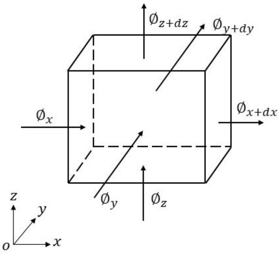
Figure 4. The microelement hexahedron.

Assuming that there is a heat source inside the object, the differential equation of the heat conduction for a unit body is given by [27] as follows:

$$\rho c\frac{\partial t}{\partial \tau }=\lambda \left(\frac{{\partial }^{2}t}{\partial x^2}+\frac{{\partial }^{2}t}{\partial y^2}+\frac{{\partial }^{2}t}{\partial z^2}\right)+q_v,$$

(20)

where $q_v$ is the internal heat source density.

The simplest initial condition is an initial uniform distribution of initial temperature, which is given by [27] as follows:

$$t=f\left(x,y,z,\tau \right)=t_0 \left(Constant\right),$$

(21)

The boundary conditions are used to guide the temperature distribution of a hot object, which can generally be divided into three categories.

• The temperature distribution at any time on the boundary of a given heat conductor [27].

$$t=t\left(x,y,z,\tau \right)\left(On the boundary of {\Gamma }_1\right)$$

(22)

The temperature is uniformly distributed at the boundary [27].

$$t=t\left(\tau \right)\left(On the boundary of {\Gamma }_1\right)$$

(23)

b.

The heat flux density at any time on the boundary of a given heat conductor [27].

$${\lambda }_x\frac{\partial t}{\partial x}{n}_x+{\lambda }_y\frac{\partial t}{\partial y}{n}_{xy}+{\lambda }_z\frac{\partial t}{\partial z}{n}_z=q\left(x,y,z,\tau \right) \left(On the boundary of {\Gamma }_2\right)$$

(24)

The heat flux density is uniformly distributed at the boundary [27].

$${\lambda }_x\frac{\partial t}{\partial x}{n}_x+{\lambda }_y\frac{\partial t}{\partial y}{n}_{xy}+{\lambda }_z\frac{\partial t}{\partial z}{n}_z=q\left(\tau \right) \left(On the boundary of {\Gamma }_2\right)$$

(25)

c.

The convective heat transfer coefficient $h$ between the boundary of the thermal conductor and the surface fluid, and the temperature of the surface fluid $t_{B }$ are given [27].

$${\lambda }_x\frac{\partial t}{\partial x}{n}_x+{\lambda }_y\frac{\partial t}{\partial y}{n}_{xy}+{\lambda }_z\frac{\partial t}{\partial z}{n}_z=h\left(t_B-t\right) \left(On the boundary of {\Gamma }_3\right)$$

(26)

The fluid temperature $t_B$ and the convective heat transfer coefficient $h$ at the boundary interface are known, while the temperature $t$ and temperature change rate $\frac{\partial t}{\partial n}$ at the boundary interface are unknown.

Assuming the temperature field solution domain is $\Omega$, and $\Gamma ={\Gamma }_1+{\Gamma }_2+{\Gamma }_3$, $\Gamma$ is the entire boundary of the domain $\Omega$.

The transient temperature field is given by [27] as follows:

$$t\left(x,y,z,0\right)=t\left(x,y,z\right).$$

(27)

When $\frac{\partial t}{\partial \tau }=0$, the steady heat conduction equation is given by [27].

$$\frac{\partial }{\partial x}({\lambda }_x\frac{\partial t}{\partial x})+\frac{\partial }{\partial y}\left({\lambda }_y\frac{\partial t}{\partial y}\right)+\frac{\partial }{\partial z}\left({\lambda }_z\frac{\partial t}{\partial z}\right)+q_v=0 \left(In \Omega \right).$$

(28)

When the thermal boundary condition and the heat generation rate are known, the temperature field distribution of the hexahedral microelement can be calculated and used for finite element modeling.

During the movement of the CNCMT spindle, heat conduction exists among the parts of the CNCMT spindle system. It is most evident in the nut and bearing seat. Therefore, the temperature fields under the heat source of the nut and bearing seat are calculated, respectively. The temperature field under a nut heat source is obtained iteratively by Equation (29) [27].

$$\begin{array}{l}\left\{\begin{array}{c}\Delta Q\left(t\right)=Q_n\left(t\right)-Q_c\left(t\right)-Q_t\left(t\right)\\ \begin{array}{c}\Delta Q\left(t\right)=c\rho L_{i}S\Delta T_{L_i}\left(t\right)\\ \begin{array}{c}\begin{array}{c}{Q}_n=0.12\pi f_w{v}_{0}n{M}_w\\ Q_c\left(t\right)=h\times S\prime \times \left(T_{L_i}\left(t\right)-T_f\left(t\right)\right)\Delta t\end{array}\\ Q_t\left(t\right)=\lambda \times S\times \frac{\left(T_{L_i}\left(t\right)-T_{L_{i+1}}\left(t\right)\right)+\left(T_{L_i}\left(t\right)-T_{L_{i-1}}\left(t\right)\right)}{L}\times \Delta t\end{array}\end{array}\end{array}\right.\end{array}$$

(29)

where $\Delta Q$ represents the $L_i$′ D-value between the generated heat and the dissipation heat; $Q_n$ represents the frictional heat generation of $L_i$; $Q_c$ represents the heat transfer rate between $L_i$ and the environment; $Q_t$ represents the heat conduction between $L_i$ and two side elements $t$; $c$ represents the lead screw specific heat capacity; $\rho$ represents the lead screw density; $S$ represents the lead screw equivalent cross-sectional area; $T_{L_i}\left(t\right)$ represents the $L_i$′s temperature rise; $f_w$ represents the coefficient associated with the screw-nut class and lubrication method; $v_0$ represents the kinematic viscosity; $n$ represents the lead screw rotational speed; $h$ represents the convective heat transfer coefficient; $S\prime$ represents $L_i$′s convective heat transfer area; $T_f\left(t\right)$ represents the air temperature around the lead screw, which approximately replaces with the temperature $T_b$ of the bed; $\lambda$ represents the lead screw thermal conductivity.

The temperature field of the bearing block under the heat source is given by [27] as follows:

$${\Gamma }_{br}\left(P_y,t\right)=\left(\chi e^{-\sqrt{\frac{2h}{kR}}{P}_y}+\zeta e^{-\sqrt{\frac{2h}{kR}}{P}_y}\right)\times \left(1-e_f\left(\frac{P_y}{2\sqrt{\alpha t}}\right)\right),$$

(30)

where $T_{br}$ represents the bearing block temperature; $P_y$ represents the distance from the heat source on the lead screw; $\chi$ and $\zeta$ are the unidentified coefficient; $k$ represents the thermal conductivity; $R$ represents the lead screw radius; $\alpha$ represents the lead screw thermal conductivity; $e_f\left(P_y\right)$ is given by [27] as follows:

$$e_f\left(P_y\right)=\frac{2}{\sqrt{\pi }}{\displaystyle {\int }_0^{P_y}{e}^{-{\lambda }^2}d\lambda }.$$

(31)

Under the joint action of the lead screw nut and the heat source of the bearing seat, the thermal error at any time $t$ is given by [27] as follows:

$$E\left(t\right)={\displaystyle \sum _{i=1}^M{\lambda }_s}\times \left(\Delta T_{L_i}\left(t\right)+\Delta {\Gamma }_{br}\left(t\right)\right)\times L_i,$$

(32)

where ${\lambda }_s$ represents the thermal expansion coefficient; $M$ represents the discrete segment number of the lead screw.

3.

Mathematical model of the thermal deformation field

Figure 5 and Figure 6 show the structural diagram and the thermal elongation of the CNCMT spindle, respectively. $B_1{B}_2$ and $L_1$ are the distance of two bearings of the CNCMT spindle. $W{B}_1$ and $L_2$ are the distance of a bearing and a mandrel. Because of the uneven temperature distribution of the CNCMT spindle system, the thermal deformation satisfies the following relationship [28].

$$\Delta L=\alpha {{\displaystyle \int }}_0^{l}T\left(x\right)dx,$$

(33)

where $\Delta x$ represents the elongation of the spindle; $\alpha$ represents the linear expansion coefficient; $l$ represents the length of the main shaft; $T\left(x\right)$ represents the CNCMT spindle temperature distribution function. $T\left(x\right)=T_{max}\left(x/L_2\right)$. $T_{max}$ is the temperature at B₁.

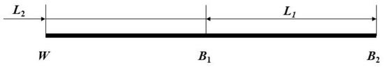
Figure 5. The structural diagram of the CNCMT spindle.

Figure 6. The thermal elongation of the CNCMT spindle.

(2)

The implementation of the LSTM model

Figure 7 shows the specific implementation process of LSTM. The inputs of the thermal error model are the screw-nut temperature, bearing temperature, ambient temperature, and motor temperature. First, it is necessary to preprocess the data. Then, the preprocessed data is separated into the training group and the test group. Next, we normalize the feature data. Finally, an LSTM network is constructed and trained to predict thermal error.

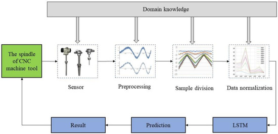
Figure 7. The implementation process of LSTM model.

(3)

The implementation of DT-LSTM

Using the fusion method, the output of LSTM is taken as the systematic observation value to correct the theoretical and empirical derivation results driven by the DT model. The PSO used in this paper is a fusion algorithm. The steps of DT-LSTM are shown in Figure 8.

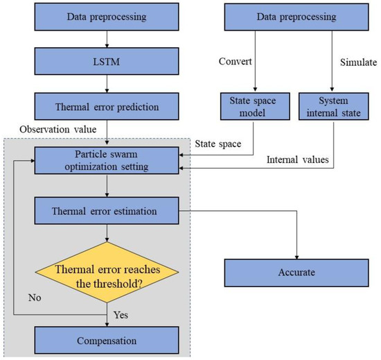
Figure 8. The steps of DT-LSTM.

• An LSTM model for the CNCMT spindle system is established, and the predicted thermal error obtained from the model is used as an observation value.
• According to the temperature variation rules in the DT model, it is converted into a temperature space model for initialization based on the fusion algorithm, and the internal state of the system is calculated using model simulation.
• The fusion algorithm is initialized based on the temperature space model, and the observed values are used to modify the theoretical values obtained from the system model simulation and reasoning. We can obtain more accurate thermal error prediction values.
• We judge whether the thermal error reaches the threshold value based on the analysis results of the fusion algorithm. If the thermal error reaches the threshold value, we should make appropriate compensation. Otherwise, return to ii to repeat the iteration.

4. Case Study

4.1. Design of Experiment Platform

Figure 9 shows that the CNCMT spindle system is composed of the motor, coupling, bearing, lead screw, and screw-nut. The motor provides the power for the feed system. The coupling links the motor and the lead screw to transmit torque. The bearings at both ends support the rotation of the lead screw. The lead screw and screw-nut comprise a lead–screw-nut pair. It enables the conversion from rotary motion to linear motion. The guide rail drives the workbench to perform the linear motion.

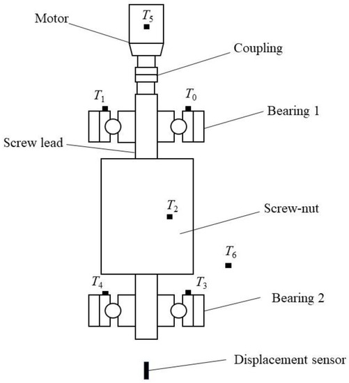
Figure 9. The structure of the CNCMT spindle system.

Seven STT-Pt100 temperature sensors are arranged on the CNCMT spindle system to measure the temperature changes. To obtain the measurement value of the axial thermal deformation, we arrange a displacement sensor on the CNCMT spindle’s Z-end. The CNCMT speed is 2000 r/min. The temperature point locations are shown in Table 1.

Table 1. The location of temperature measuring points.

T0	T1	T2	T3	T4	T5	T6
Bearing 1	Bearing 1	Screw-nut	Bearing 2	Bearing 2	Motor	Surrounding

4.2. The Optimization of the Temperature Measurement Points

The optimized temperature measurement points can reduce the temperature variables. Meanwhile, it can reduce the model computing resources and improve the model computing accuracy. We use the fuzzy clustering method to optimize the temperature measurement points. The specific method is seen in the literature [29]. We set the number of the cluster center as five. The iteration times are set to 100. The convergence precision is set to 1 × 10⁻⁶. The blur coefficient is set to two. Therefore, the grouping results of the temperature data can be obtained. Seven temperature measurement points are divided into five groups: T₀, T₁; T₂; T₃, T₄; T₅; T₆.

Based on the above grouping results, we use statistical theory to optimize the temperature measurement points. We use the similarity coefficient method to calculate the correlation coefficient between each temperature measurement point and the thermal error [29].

$$r_{x_{i}E}=\frac{{\displaystyle \sum _{j=1}^n\left(x_{ij}-\overline{x_i}\right)\left(E_j-\overline{E}\right)}}{\sqrt{{\displaystyle \sum _{J=1}^n{\left(x_{ij}-\overline{x_i}\right)}^2}}\sqrt{{\displaystyle \sum _{J=1}^n{\left(E_j-\overline{E}\right)}^2}}},$$

(34)

where $r_{x_{i}E}$ represents the correlation coefficient; $x_{ij}$ represents the measuring point temperature; $i$ represents the i-th measuring point, totaling $m$ measuring points; $j$ represents the measurement number at the same measuring point; $n$ represents the measurement number at the same measuring point; $x_i$ represents the average temperature of all $n$ measurements at the measurement point $i$; $\overline{E}$ represents the average thermal error of all measured values at the same measuring point; $E_j$ represents the j-th thermal error measurement value.

Through the calculation of Equation (34), we can obtain the correlation coefficient of each temperature measurement point. The correlation coefficients are shown in Table 2. Figure 10 shows the correlation curve of “E—x”.

Table 2. The correlation coefficient of temperature measurement points.

Temperature Measurement Point	Correlation Coefficient	Temperature Measurement Point	Correlation Coefficient
T0	0.9498	T4	0.9565
T1	0.9489	T5	0.8866
T2	0.9503	T6	0.8815
T3	0.9555

Figure 10. The correlation curve of “E—x”.

Comparing the coefficients of each group, we select the optimal temperature measurement point of each group. From the values of the correlation coefficients in Table 2, we select T₀, T₂, T₄, T₅, and T₆ as the temperature input data for the thermal error modelling.

4.3. DT-LSTM-based Thermal Error Prediction Approach for CNCMT Spindle

4.3.1. The Realization of the DT Model

In order to construct a DT model of the CNCMT spindle system, Table 3 shows the material parameters of the CNCMT spindle system.

Table 3. The material parameters of the CNCMT spindle system.

Part	Spindle	Bearing
Material	GCr15SiMn	GCr15
Density/(kg/m3)	7810	7830
Modulus of elasticity E/Pa	2.06 × 1011	2.19 × 1011
Poisson’s ratio μ	0.3	0.3
Specific heat capacity C/(J·(kg·K)−1)	460	160
Thermal conductivity/(W·(m·K)−1)	60.5	81
Coefficient of thermal expansion	1.2 × 10−5	1.25 × 10−5

To facilitate the establishment of the DT model of the CNCMT spindle system, we use UG software to appropriately simplify the three-dimensional model of the spindle (e.g., smaller holes, non-critical grooves, smaller fillets, and chamfers). The simplified model is imported into Workbench software. Then, in order to simplify the calculation process, a two-dimensional axisymmetric model is drawn based on the cross-sectional dimensions. Finally, to ensure the convergence of the entire model and the accuracy of the temperature distribution results, the grid division of the heat transfer concentration area near the bearing is relatively dense, and the grid division of the inner cavity and outer surface edge areas of the spindle is relatively sparse. After adding temperature measuring points, the DT system starts to measure the spindle temperature and correct the thermal boundary. Figure 11 shows the temperature field of the CNCMT spindle system at 60 min. Figure 12 shows the thermal deformation field of the CNCMT spindle system at 60 min.

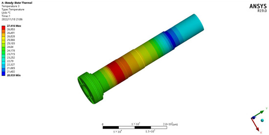
Figure 11. The temperature field of the CNCMT spindle.

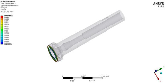
Figure 12. The thermal deformation field of the CNCMT spindle’s Z-end.

Figure 13, Figure 14, Figure 15, Figure 16 and Figure 17 show the temperature rise at the key temperature measurement points. Figure 18 shows a comparison between the simulated thermal deformation and the actual thermal deformation of the spindle’s Z-end. We can see that the simulated temperature accuracy of DT is above 98%, and the thermal deformation simulation accuracy is up to 95%. It proves that the spindle DT model can reflect the actual thermal characteristics.

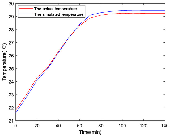
Figure 13. The temperature rise of T₀.

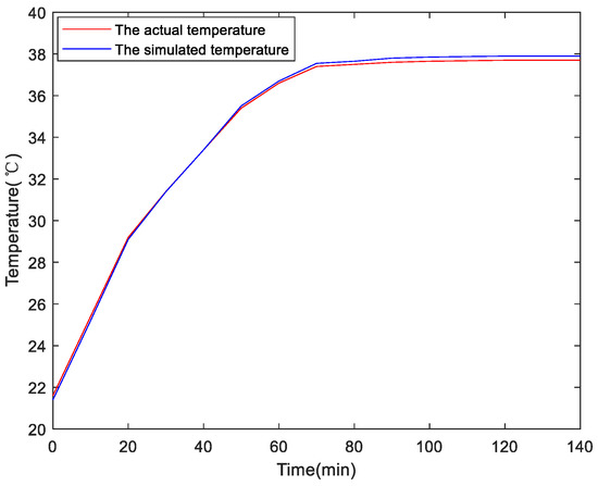
Figure 14. The temperature rise of T₂.

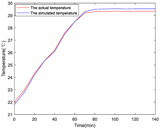
Figure 15. The temperature rise of T₄.

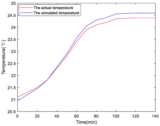
Figure 16. The temperature rise of T₅.

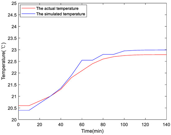
Figure 17. The temperature rise of T₆.

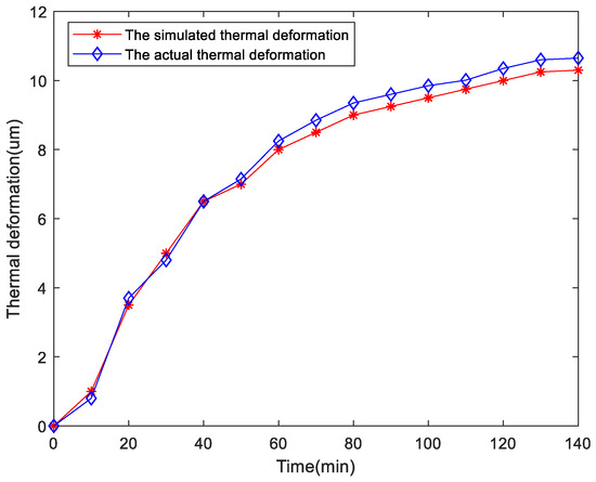
Figure 18. The thermal deformation of CNCMT spindle’s Z-end.

4.3.2. The Realization of the LSTM Model

First, we smooth the collected data. Taking temperature data as an example, Figure 19 depicts one of the collected temperature data. The curve has a lot of noise. Therefore, it needs to be smoothed. To reduce computational complexity, we adopt the moving average filtering method. The result of smoothing is shown in Figure 20. After noise elimination, we chose 70% for the training group and 30% for the test group. The normalization formula is givenby [30,31].

$$x_i^{\prime }=\frac{x_i-x_{\min }}{x_{\max }-x_{miin}}$$

(35)

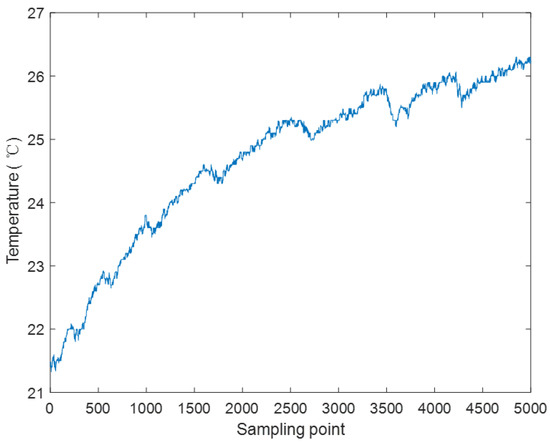
Figure 19. The collected temperature data.

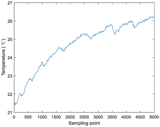
Figure 20. The collected temperature data after smoothing.

This paper builds an LSTM neural network based on the Python framework. Due to the complexity and depth of the model structure, it is necessary to simplify the model structure. In order to select a suitable model structure, we conduct the relevant experiments. As shown in Table 4, we can obtain the maximum residual error by setting different LSTM layers and hidden node numbers. The maximum residual error of the LSTM with two layers and twelve hidden nodes is the smallest, which has the highest accuracy.

Table 4. The maximum residual error corresponding to different LSTM layers and hidden node numbers.

Model Structure	LSTM Two-Layer Maximum Residual Error (μm)	LSTM Three-Layer Maximum Residual Error (μm)	LSTM Four-Layer Maximum Residual Error (μm)
eight hidden nodes	10.5	7	16
twelve hidden nodes	6	9.5	19
sixteen hidden nodes	8	11.5	24.2
twenty hidden nodes	9.6	10	16.7

After repeated experiments, we choose the LSTM structure with four layers, which includes one input layer, two hidden layers, one output layer, six input layer nodes, twelve hidden layer nodes, and two output layer nodes. We use the gradient descent method to find the optimal solution, and the training results display the maximum residuals of the predicted value. We set the number of iterations as 1000 and the learning rate as 0.1. The model parameters are randomly initialized. The root mean square error (RMSE) convergence curve during training is shown in Figure 21.

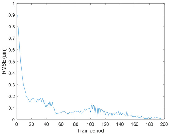
Figure 21. The RMSE convergence curve of LSTM.

4.3.3. The Realization of DT-LSTM

Equation (32) shows the theoretical value of the CNCMT spindle thermal error, which is used as the system state equation in the PSO to initialize the algorithm. Meanwhile, the actual value of the thermal error obtained by LSTM is shown in Equation (6), which is used as the system observation value in the PSO.

The number of particles is set to 150. The DT-LSTM Algorithm 1 is shown below.

Algorithm 1. DT-LSTM for the CNCMT spindle’s thermal error prediction

Input: The theoretical prediction value of DT and the actual prediction value of LSTM

Output: The particles prediction value

(1) Initialize the parameters and particles

(2) $E\left(t\right)={\displaystyle \sum _{i=1}^M{\lambda }_s}\times \left(\Delta T_{L_i}\left(t\right)+\Delta {\Gamma }_{br}\left(t\right)\right)\times L_i$

(3) $h_t=o_t\cdot \tanh \left(C_t\right)$ for 1 = 1:150

(4) Sample from (2)

(5) Calculate the thermal error prediction value ${\mathrm{h}}_{ti}$ of particles by (3)

(6) Calculate the weight $E(i)$ of each particleend

(7) Normalize the weight

(8) Resample according to the normalized weight

(9) Output the CNCMT spindle’s thermal error prediction value $h_f$

4.4. The Analysis of Experiment Result

The thermal prediction value of different methods is shown in Figure 22. Figure 23 shows the comparison of different hybrid algorithms, which proves the superior performance of PSO. When we use single prediction methods (e.g., DT and LSTM), there is a significant error between the predicted curve and the actual curve. When we use DT-LSTM, the predicted curve is close to the actual curve, and the prediction accuracy is improved. DT-LSTM overcomes the model inconsistency of DT and the poor adaptability of LSTM. DT-LSTM has higher accuracy than the single method by nearly 11%, which improves the prediction performance and robustness of thermal error. Table 5 shows the quantitative evaluation of different methods. Table 6 shows the accuracy comparison of different methods. The result indicates that DT-LSTM has a higher accuracy at all stages compared with DT and LSTM. The average accuracy of LSTM is 98%. Meanwhile, DT-LSTM shows better prediction performance compared with the other method.

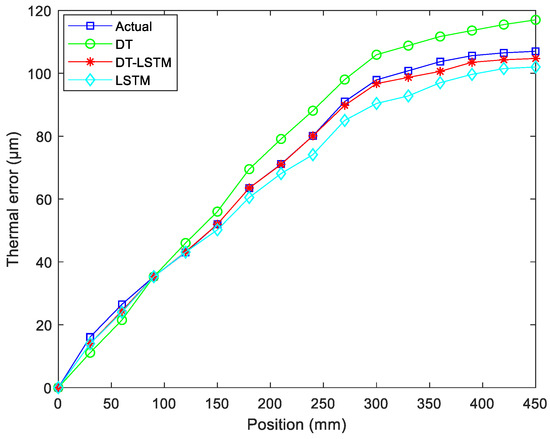
Figure 22. The thermal prediction value of different methods.

Figure 23. The comparison of different hybrid algorithms.

Table 5. The quantitative evaluation of different methods.

	Start Stage Accuracy	Middle Stage Accuracy	End Stage Accuracy	Average Accuracy
DT	91%	88%	82%	87%
LSTM	98%	90%	85%	91%
DT-LSTM	100%	99%	95%	98%

Table 6. The accuracy comparison of different methods.

Method	Accuracy
Co-Simulation-Based DT [18]	96%
SVM [14]	97.16%
DT-LSTM	98%

5. Conclusions

To enhance the prediction performance of CNCMT spindle thermal error, we propose a novel thermal error prediction method using DT-LSTM. Firstly, we establish a DT system to simulate the CNCMT spindle thermal characteristics. Based on the simulated result, we can obtain the theoretical value of thermal error. Then, LSTM is constructed to analyze the experimental data. The output of LSTM is the actual value of thermal error. Finally, we use the particle swarm optimization algorithm to fuse the theoretical values of DT with the actual values of LSTM. DT-LSTM is compared with the single method, and the accuracy of DT-LSTM is greater than 98%. Therefore, DT-LSTM can predict the CNCMT spindle thermal error effectively and provide a theoretical basis for the CNCMT spindle thermal error compensation. This paper only verifies the method for the spindle. In the future, DT-LSTM will be applied to the other components of CNCMT. Real time is a crucial aspect of thermal error prediction. The simulation of the DT physical performance model consumes many computing resources and time. In the future, we will improve the real-time performance and computational efficiency of DT simulation.

References

- Li, Y.; Tian, H.; Liu, D.; Lu, Q.B. Thermal error analysis of five-axis machine tools based on five-point test method. Lubricants 2022, 10, 122. [Google Scholar] [CrossRef]
- Peng, J.; Yin, M.; Cao, L.; Liao, Q.; Wang, L.; Yin, G. Study on the spindle axial thermal error of a five-axis machining center considering the thermal bending effect. Precis. Eng. 2022, 75, 210–226. [Google Scholar] [CrossRef]
- Ouerhani, N.; Loehr, B.; Rizzotti-Kaddouri, A.; Santo De Pinho, D.; Limat, A.; Schinderholz, P. Data-driven thermal deviation prediction in turning machine-tool-a comparative analysis of machine learning algorithms. Procedia Comput. Sci. 2022, 200, 185–193. [Google Scholar] [CrossRef]
- Zimmermann, N.; Lang, S.; Blaser, P.; Mayr, J. Adaptive input selection for thermal error compensation models. CIRP Ann. 2020, 69, 485–488. [Google Scholar] [CrossRef]
- Liang, Y.C.; Li, W.D.; Lou, P.; Hu, J.M. Thermal error prediction for heavy-duty CNC machines enabled by long short-term memory networks and fog-cloud architecture. J. Manuf. Syst. 2022, 62, 950–963. [Google Scholar] [CrossRef]
- Li, Y.; Yu, M.; Bai, Y.; Hou, Z.; Wu, W. A review of thermal error modeling methods for machine tools. Appl. Sci. 2021, 11, 5216. [Google Scholar] [CrossRef]
- Li, Z.; Wang, B.; Zhu, B.; Wang, Q.; Zhu, W. Thermal error modeling of electrical spindle based on optimized ELM with marine predator algorithm. Case Stud. Therm. Eng. 2022, 38, 102326. [Google Scholar] [CrossRef]
- Liao, Q.; Yin, Q.; Xie, L.; Yin, G. Improved exponential model for thermal error modeling of machine-tool spindle based on fruit fly optimization algorithm. Proc. Inst. Mech. Eng. C J. Mech. 2022, 236, 6912–6922. [Google Scholar] [CrossRef]
- Kumar, T.S.; Kurian, C.P. Real-time data based thermal comfort prediction leading to temperature setpoint control. J. Ambient Intell. Hum. Comput. 2022, 1–12. [Google Scholar] [CrossRef]
- Li, Z.; Fan, K.; Yang, J.; Zhang, Y. Time-varying positioning error modeling and compensation for ball screw systems based on simulation and experimental analysis. Int. J. Adv. Manuf. Technol. 2014, 73, 773–782. [Google Scholar] [CrossRef]
- Abdulshahed, A.M.; Longstaff, A.P.; Fletcher, S.; Potdar, A. Thermal error modelling of a gantry-type 5-axis machine tool using a grey neural network model. J. Manuf. Syst. 2016, 41, 130–142. [Google Scholar] [CrossRef]
- Zhu, X.; Liu, Q.; Zhang, X.; Jiang, X.; Lou, P. Robustness analysis of the thermal error model for a CNC machine tool. In Proceedings of the 2016 8th International Conference on Intelligent Human-Machine Systems and Cybernetics (IHMSC), Cairo, Egypt, 27–28 August 2016; pp. 510–513. [Google Scholar]
- Yang, J.; Zhang, D.; Mei, X.; Zhao, L.; Ma, C.; Shi, H. Thermal error simulation and compensation in a jig-boring machine equipped with a dual-drive servo feed system. Proc. Inst. Mech. Eng. B J. Eng. 2015, 229, 43–63. [Google Scholar] [CrossRef]
- Liu, J.; Gui, H.; Ma, C. Digital twin system of thermal error control for a large-size gear profile grinder enabled by gated recurrent unit. J. Ambient Intell. Hum. Comput. 2023, 14, 1269–1295. [Google Scholar] [CrossRef]
- Ma, C.; Gui, H.; Liu, J. Self learning-empowered thermal error control method of precision machine tools based on digital twin. J. Intell. Manuf. 2023, 34, 695–717. [Google Scholar] [CrossRef]
- Xiao, J.; Fan, K. Research on the digital twin for thermal characteristics of motorized spindle. Int. J. Adv. Manuf. Technol. 2022, 119, 5107–5118. [Google Scholar] [CrossRef]
- Liu, K.; Song, L.; Han, W.; Cui, Y.; Wang, Y. Time-varying error prediction and compensation for movement axis of CNC machine tool based on digital twin. IEEE Trans. Ind. Inform. 2021, 18, 109–118. [Google Scholar] [CrossRef]
- Yi, H.; Fan, K. Co-simulation-based digital twin for thermal characteristics of motorized spindle. Int. J. Adv. Manuf. Technol. 2023, 125, 4725–4737. [Google Scholar] [CrossRef]
- Liu, J.; Ma, C.; Gui, H.; Wang, S. A four-terminal-architecture cloud-edge-based digital twin system for thermal error control of key machining equipment in production lines. Mech. Syst. Signal Process. 2022, 166, 108488. [Google Scholar] [CrossRef]
- Lunev, A.; Lauerer, A.; Zborovskii, V.; Léonard, F. Digital twin of a laser flash experiment helps to assess the thermal performance of metal foams. Int. J. Therm. Sci. 2022, 181, 107743. [Google Scholar] [CrossRef]
- Kuprat, J.; Pascal, Y.; Liserre, M. Real-Time thermal characterization of power semiconductors using a PSO-based digital twin approach. In Proceedings of the 2022 24th European Conference on Power Electronics and Applications (EPE’22 ECCE Europe), Hanover, Germany, 5–9 September 2022; pp. 1–8. [Google Scholar]
- Liu, R.J.; Li, H.S.; Lv, Z.H. Modeling methods of 3D model in digital twins. CMES Comp. Model. Eng. 2023, 136, 985–1022. [Google Scholar] [CrossRef]
- Grieves, M.W. Product lifecycle management: The new paradigm for enterprises. Int. J. Prod. Dev. 2005, 2, 71–84. [Google Scholar] [CrossRef]
- Tao, F.; Zhang, H.; Liu, A.; Nee, A.Y. Digital twin in industry: State-of-the-art. IEEE Trans. Ind. Inform. 2018, 15, 2405–2415. [Google Scholar] [CrossRef]
- Smagulova, K.; James, A.P. A survey on LSTM memristive neural network architectures and applications. Eur. Phys. J. Spec. Top. 2019, 228, 2313–2324. [Google Scholar] [CrossRef]
- Korstanje, J. LSTM RNNs. In Advanced Forecasting with Python: With State-of-the-Art-Models Including LSTMs, Facebook’s Prophet, and Smazon’s DeepAR Apress; Apress: Berkeley, CA, USA, 2021; pp. 243–251. [Google Scholar]
- Pope, J.E.; Pope, E. Rule of Thumb for Mechanical Engineers-A Manual of Quick, Accurate Solutions to Everyday Mechanical Engineering Problems; Gulf Professional Publishing: Houston, TX, USA, 1997; pp. 18–50. [Google Scholar]
- Chen, Z.C.; Chen, Z.N. Termal Characteristics Foundation of Machine Tools; Machinery Industry Press: Beijing, China, 1989. [Google Scholar]
- Ruspini, E.H.; Bezdek, J.C.; Keller, J.M. Fuzzy clustering: A historical perspective. IEEE Comput. Intell. Mag. 2019, 14, 45–55. [Google Scholar] [CrossRef]
- Fang, B.; Zhang, J.; Hong, J.; Yan, K. Research on the nonlinear stiffness characteristics of double-row angular contact ball bearings under different working conditions. Lubricants 2023, 11, 44. [Google Scholar] [CrossRef]
- Ma, S.; Yin, Y.; Chao, B.; Yan, K.; Fang, B.; Hong, J. A real-time coupling model of bearing-rotor system based on semi-flexible body element. Int. J. Mech. Sci. 2023, 245, 108098. [Google Scholar] [CrossRef]
Disclaimer/Publisher’s Note: The statements, opinions and data contained in all publications are solely those of the individual author(s) and contributor(s) and not of MDPI and/or the editor(s). MDPI and/or the editor(s) disclaim responsibility for any injury to people or property resulting from any ideas, methods, instructions or products referred to in the content. |
© 2023 by the authors. Licensee MDPI, Basel, Switzerland. This article is an open access article distributed under the terms and conditions of the Creative Commons Attribution (CC BY) license (https://creativecommons.org/licenses/by/4.0/).