
Narrow Band Active Contour Attention Model for Medical Segmentation


Abstract
:1. Introduction
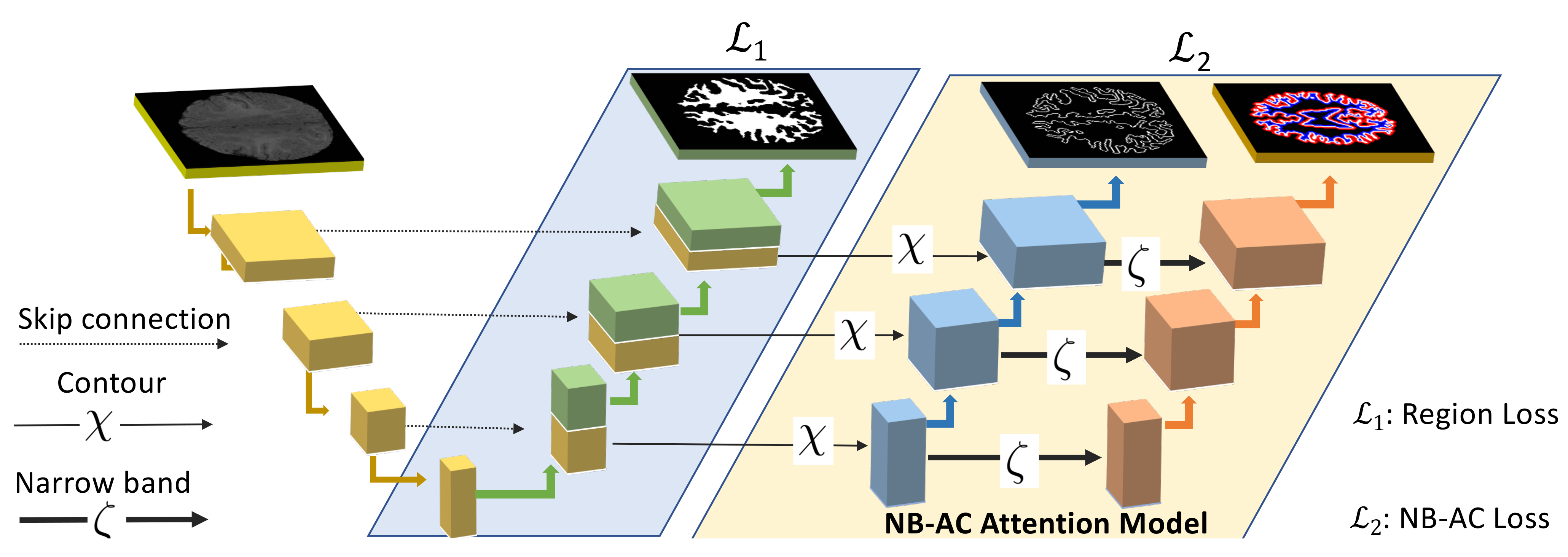
- Tackle the weak boundary object segmentation problem: the proposed NB-AC attention model is designed as an edge extractor and makes use of the narrow band principle, which has proven its efficiency in the evolution of level sets [13]. Furthermore, the proposed NB-AC loss is defined under an active contour energy minimization [10] which has been proven to be useful for weak object segmentation.
- Address the imbalanced-class data problem: instead of taking into account all pixels belonging to an image domain and assigning a label to every single pixel, the NB-AC attention model focuses on a subset of supportive pixels located within the narrow band defined by the inner band and outer band. By ignoring all pixels that are outside of the narrow band, the proposed NB-AC attention model is considered as an under-sampling approach to solve imbalanced-class data problem. In the scenario of an under-sampling solution, which removes samples from the majority class to compensate for imbalanced distribution between classes, our proposed NB-AC attention model helps answer an important question “which samples should be removed/kept?”.
- Propose a new type of transitional gate that allows the higher level feature to interact with the lower level feature in an end-to-end framework.
2. Related Works
2.1. Active Contour (AC)
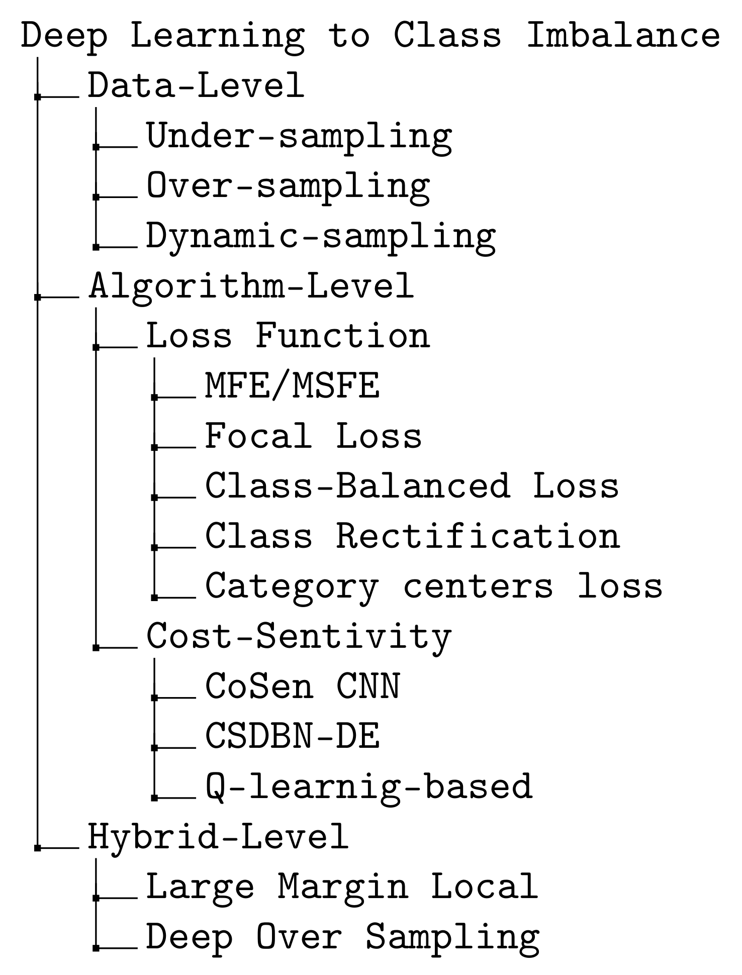
2.2. Class Imbalance
2.3. Loss Function
3. Our Proposed Two-Branch Network
3.1. Higher Level Feature Branch
3.2. Transitional Gate
3.3. Lower Level Feature Branch
3.4. Network Architecture
4. Experiments and Conclusions
4.1. Metrics
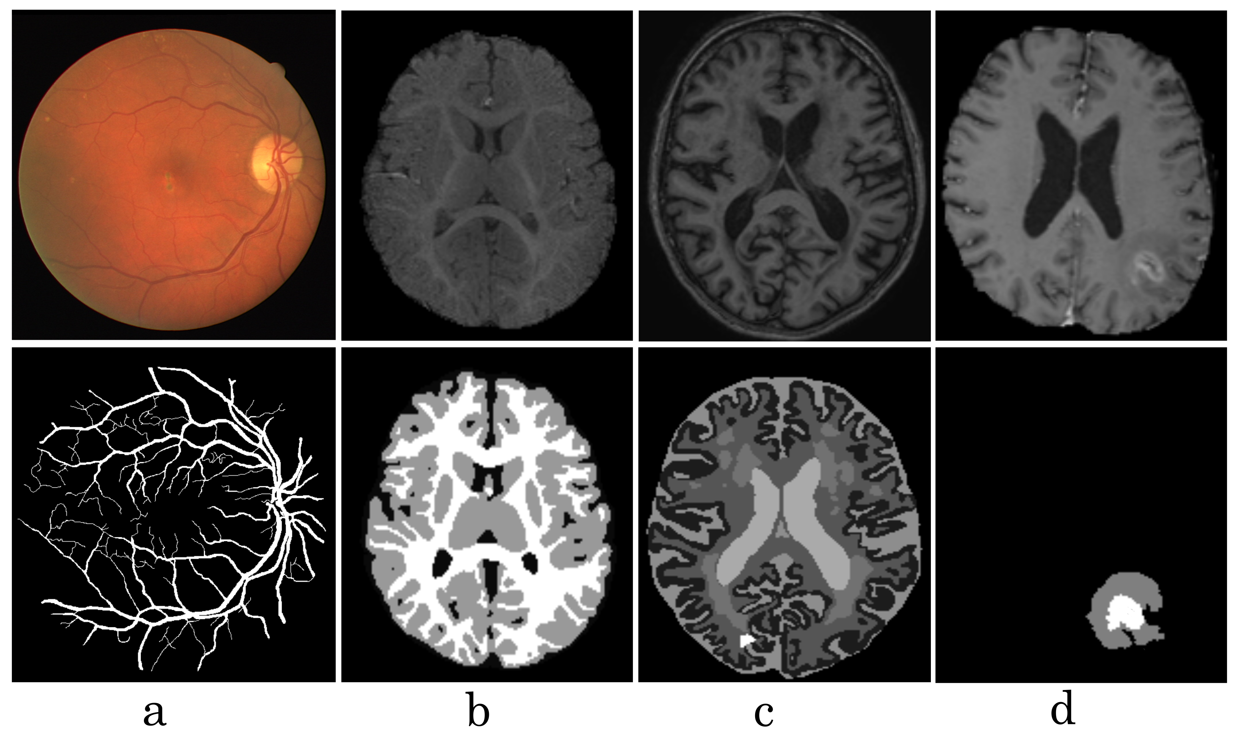
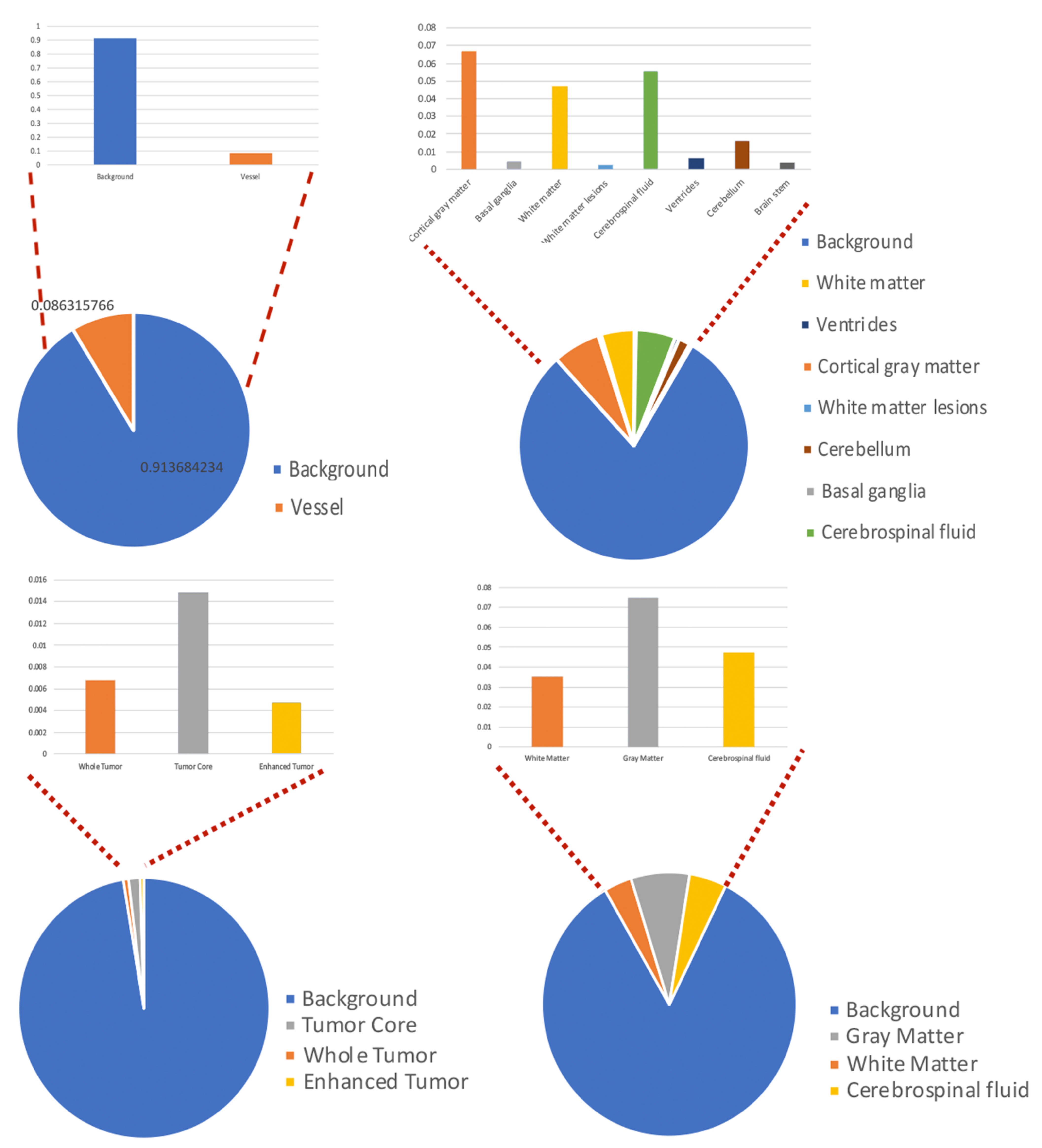
4.2. Dataset
4.3. Experiment Setting
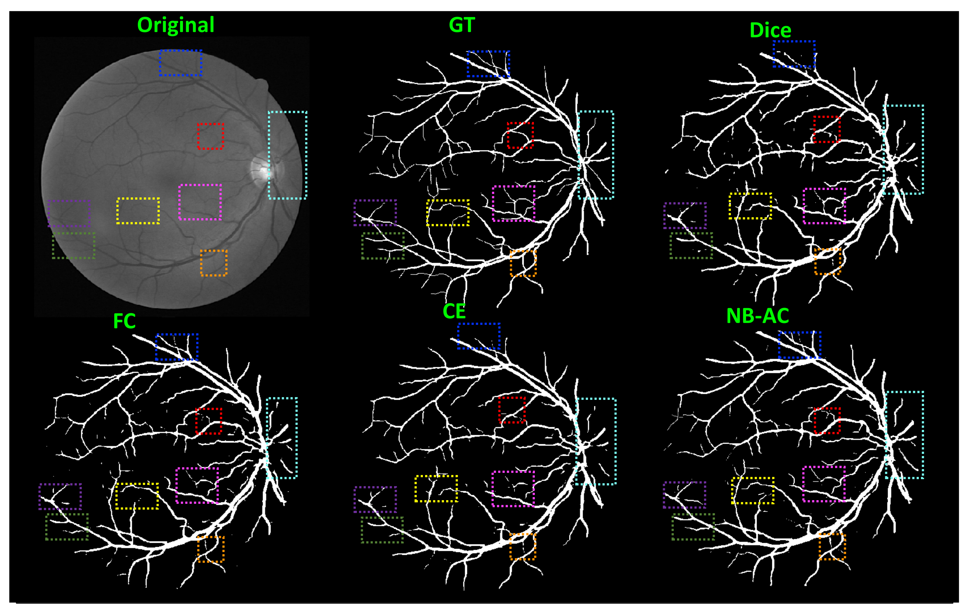
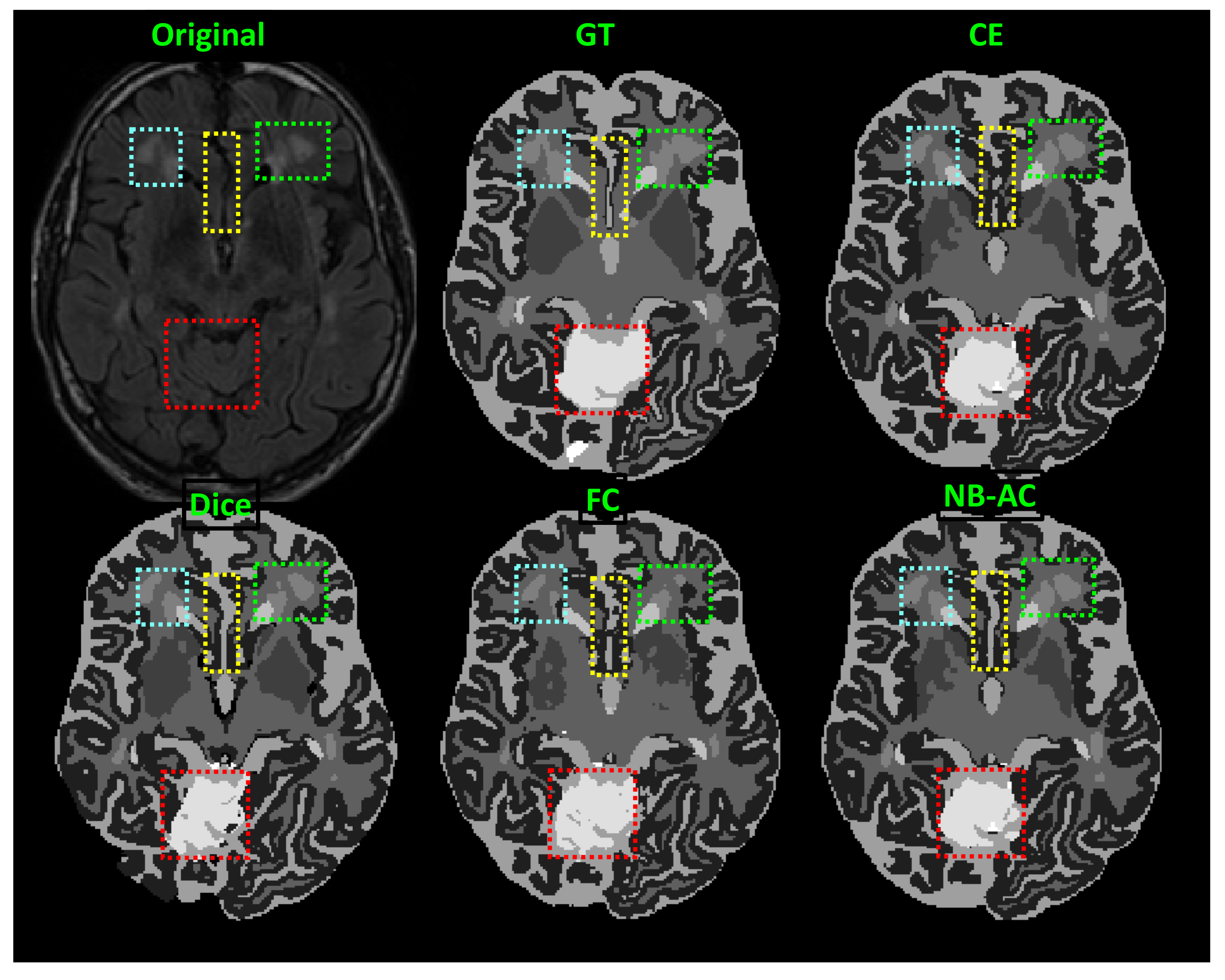
4.4. Results and Comparison
5. Conclusions
Author Contributions
Funding
Data Availability Statement
Conflicts of Interest
References
- Chen, X.; Williams, B.M.; Vallabhaneni, S.R.; Czanner, G.; Williams, R.; Zheng, Y. Learning Active Contour Models for Medical Image Segmentation. In Proceedings of the IEEE/CVF Conference on Computer Vision and Pattern Recognition (CVPR), Long Beach, CA, USA, 16–20 June 2019; pp. 11632–11640. [Google Scholar]
- Le, T.H.N.; Gummadi, R.; Savvides, M. Deep Recurrent Level Set for Segmenting Brain Tumors. In Lecture Notes in Computer Science, Proceedings of the International Conference on Medical Image Computing and Computer-Assisted Intervention, Granada, Spain, 16–20 September 2018; Frangi, A.F., Schnabel, J.A., Davatzikos, C., Alberola-López, C., Fichtinger, G., Eds.; Springer: Cham, Switzerland, 2018. [Google Scholar]
- Ronneberger, O.; Fischer, P.; Brox, T. U-net: Convolutional networks for biomedical image segmentation. In Lecture Notes in Computer Science, Proceedings of the International Conference on Medical Image Computing and Computer-Assisted Intervention, Munich, Germany, 5–9 October 2015; Springer: Cham, Switzerland, 2015; pp. 234–241. [Google Scholar]
- Çiçek, Ö.; Abdulkadir, A.; Lienkamp, S.S.; Brox, T.; Ronneberger, O. 3D U-Net: Learning Dense Volumetric Segmentation from Sparse Annotation. In Lecture Notes in Computer Science, Proceedings of the International Conference on Medical Image Computing and Computer-Assisted Intervention, Athens, Greece, 17–21 October 2016; Springer: Cham, Switzerland, 2016; pp. 424–432. [Google Scholar]
- Wang, G.; Li, W.; Ourselin, S.; Vercauteren, T. Automatic Brain Tumor Segmentation Based on Cascaded Convolutional Neural Networks With Uncertainty Estimation. Front. Comput. Neurosci. 2019, 13, 56. [Google Scholar] [CrossRef] [PubMed] [Green Version]
- Fausto, M.; Nassir, N.; Seyed-Ahmad, A. V-Net: Fully Convolutional Neural Networks for Volumetric Medical Image Segmentation. In Proceedings of the Fourth International Conference on 3D Vision, Stanford, CA, USA, 25–28 October 2016; pp. 565–571. [Google Scholar]
- Lin, T.; Goyal, P.; Girshick, R.; He, K.; Dollar, P. Focal loss for dense object detection. In Proceedings of the IEEE International Conference on Computer Vision (ICCV), Venice, Italy, 22–29 October 2017; pp. 2980–2988. [Google Scholar]
- Xu, L.; Luo, B.; Pei, Z. Weak boundary preserved superpixel segmentation based on directed graph clustering. Signal Process. Image Commun. 2018, 65, 231–239. [Google Scholar] [CrossRef]
- Le, N.; Le, T.; Yamazaki, K.; Bui, T.; Luu, K.; Savides, M. Offset Curves Loss for Imbalanced Problem in Medical Segmentation. In Proceedings of the 2020 25th International Conference on Pattern Recognition (ICPR), Milan, Italy, 13–18 September 2020; pp. 9189–9195. [Google Scholar]
- Chan, T.F.; Vese, L.A. Active Contours Without Edges. IEEE Trans. Image Process. 2001, 10, 266–277. [Google Scholar] [CrossRef] [PubMed] [Green Version]
- Mumford, D.; Shah, J. Optimal Approximation by Piecewise Smooth Functions and Associated Variational Problems. Commun. Pure Appl. Math. 1989, 42, 577–685. [Google Scholar] [CrossRef] [Green Version]
- Kervadec, H.; Bouchtiba, J.; Desrosiers, C.; Granger, E.; Dolz, J.; Ben Ayed, I. Boundary loss for highly unbalanced segmentation. In Proceedings of the 2nd International Conference on Medical Imaging with Deep Learning, London, UK, 8–10 July 2019; pp. 285–296. [Google Scholar]
- Malladi, R.; Sethian, J.A.; Vemuri, B.C. Shape modeling with front propagation: A level set approach. IEEE Trans. Pattern Anal. Mach. Intell. 1995, 17, 158–175. [Google Scholar] [CrossRef] [Green Version]
- Staal, J.; Abramoff, M.; Niemeijer, M.; Viergever, M.; van Ginneken, B. Ridge based vessel segmentation in color images of the retina. IEEE Trans. Med. Imaging 2004, 23, 501–509. [Google Scholar] [CrossRef]
- Wang, L.; Nie, D.; Li, G.; Puybareau, É.; Dolz, J.; Zhang, Q.; Wang, F.; Xia, J.; Wu, Z.; Chen, J.; et al. Benchmark on Automatic 6-month-old Infant Brain Segmentation Algorithms: The iSeg-2017 Challenge. IEEE Trans. Med. Imaging 2019, 38, 2219–2230. [Google Scholar] [CrossRef] [Green Version]
- MR Brain Segmentation at MICCAI 2018. Available online: http://mrbrains18.isi.uu.nl/ (accessed on 1 July 2021).
- Menze, B.H.; Jakab, A.; Bauer, S.; Kalpathy-Cramer, J.; Farahani, K.; Kirby, J.; Burren, Y.; Porz, N.; Slotboom, J.; Wiest, R.; et al. The multimodal brain tumor image segmentation benchmark (BRATS). IEEE Trans. Med. Imaging 2015, 34, 1993–2024. [Google Scholar] [CrossRef]
- Li, C.; Huang, R.; Ding, Z.; Gatenby, C.; Metaxas, D.N.; Gore, J.C. A Level Set Method for Image Segmentation in the Presence of Intensity Inhomogene ities with Application to MRI. IEEE Trans. Image Process. 2011, 20, 2007–2016. [Google Scholar]
- Le, T.H.N.; Savvides, M. A Novel Shape Constrained Feature-based Active Contour (SC-FAC) Model for Lips/Mouth Segmentationin the Wild. Pattern Recognit. 2016, 54, 23–33. [Google Scholar] [CrossRef]
- Anand, R.; Mehrotra, K.G.; Mohan, C.K.; Ranka, S. An improved algorithm for neural network classification of imbalanced training sets. IEEE Trans. Neural Netw. 1993, 4 6, 962–969. [Google Scholar] [CrossRef] [Green Version]
- Lee, H.; Park, M.; Kim, J. Plankton classification on imbalanced large scale database via convolutional neural networks with transfer learning. In Proceedings of the 2016 IEEE International Conference on Image Processing (ICIP), Phoenix, AZ, USA, 25–28 September 2016; pp. 3713–3717. [Google Scholar]
- Masko, D.; Hensman, P. The Impact of Imbalanced Training Data for Convolutional Neural Networks. 2015. Available online: https://www.kth.se/social/files/588617ebf2765401cfcc478c/PHensmanDMasko_dkand15.pdf (accessed on 1 July 2021).
- Pouyanfar, S.; Tao, Y.; Mohan, A.; Tian, H.; Kaseb, A.; Gauen, K.; Dailey, R.; Aghajanzadeh, S.; Lu, Y.; Chen, S.; et al. Dynamic Sampling in Convolutional Neural Networks for Imbalanced Data Classification. In Proceedings of the 2018 IEEE Conference on Multimedia Information Processing and Retrieval (MIPR), Miami, FL, USA, 10–12 April 2018; pp. 112–117. [Google Scholar]
- Wang, S.; Liu, W.; Wu, J.; Cao, L.; Meng, Q.; Kennedy, P.J. Training deep neural networks on imbalanced data sets. In Proceedings of the 2016 International Joint Conference on Neural Networks (IJCNN), Vancouver, BC, Canada, 24–29 July 2016; pp. 4368–4374. [Google Scholar]
- Dong, Q.; Gong, S.; Zhu, X. Class Rectification Hard Mining for Imbalanced Deep Learning. In Proceedings of the 2017 IEEE International Conference on Computer Vision (ICCV), Venice, Italy, 22–29 October 2017; pp. 1869–1878. [Google Scholar]
- Khan, S.H.; Hayat, M.; Bennamoun, M.; Sohel, F.A.; Togneri, R. Cost-Sensitive Learning of Deep Feature Representations From Imbalanced Data. IEEE Trans. Neural Netw. Learn. Syst. 2018, 29, 3573–3587. [Google Scholar]
- Zhang, C.; Tan, K.C.; Ren, R. Training cost-sensitive Deep Belief Networks on imbalance data problems. In Proceedings of the 2016 International Joint Conference on Neural Networks (IJCNN), Vancouver, BC, Canada, 24–29 July 2016; pp. 4362–4367. [Google Scholar]
- Cui, Y.; Jia, M.; Lin, T.Y.; Song, Y.; Belongie, S. Class-Balanced Loss Based on Effective Number of Samples. In Proceedings of the 2019 IEEE/CVF Conference on Computer Vision and Pattern Recognition (CVPR), Long Beach, CA, USA, 15–20 June 2019. [Google Scholar]
- Huang, C.; Li, Y.; Loy, C.C.; Tang, X. Learning Deep Representation for Imbalanced Classification. In Proceedings of the 2016 IEEE/CVF Conference on Computer Vision and Pattern Recognition (CVPR), Las Vegas, NV, USA, 27–30 June 2016; pp. 5375–5384. [Google Scholar]
- Ando, S.; Huang, C.Y. Deep over-sampling framework for classifying imbalanced data. In Proceedings of the Joint European Conference on Machine Learning and Knowledge Discovery in Databases, Skopje, Macedonia, 18–22 September 2017; pp. 770–785. [Google Scholar]
- Zhang, Y.; Shuai, L.; Ren, Y.; Chen, H. Image classification with category centers in class imbalance situation. In Proceedings of the 2018 33rd Youth Academic Annual Conference of Chinese Association of Automation (YAC), Nanjing, China, 18–20 May 2018; pp. 359–363. [Google Scholar]
- Lin, E.; Chen, Q.; Qi, X. Deep Reinforcement Learning for Imbalanced Classification. arXiv 2019, arXiv:1901.01379. [Google Scholar] [CrossRef] [Green Version]
- Murphy, K.P. Machine Learning: A Probabilistic Perspective; MIT Press: Cambridge, MA, USA, 2012. [Google Scholar]
- Sudre, C.H.; Wenqi, L.; Tom, V.; Sebastien, O.; Cardoso, M.J. Generalised Dice Overlap as a Deep Learning Loss Function for Highly Unbalanced Segmentations. In DLMI and MLCS: Deep Learning in Medical Image Analysis and Multimodal Learning for Clinical Decision; Springer: Cham, Switzerland, 2017; pp. 240–248. Available online: https://link.springer.com/chapter/10.1007%2F978-3-319-67558-9_28 (accessed on 1 July 2021).
- Long, J.; Shelhamer, E.; Darrell, T. Fully convolutional networks for semantic segmentation. In Proceedings of the Conference on Computer Vision and Pattern Recognition, Boston, MA, USA, 7–12 June 2015; pp. 3431–3440. [Google Scholar]
- Gray, A.; Abbena, E.; Salamon, S. Modern Differential Geometry of Curves and Surfaces with Mathematica; Chapman and Hall/CRC Press: Boca Raton, FL, USA, 2006. [Google Scholar]
- Mille, J. Narrow Band Region-Based Active Contours and Surfaces for 2D and 3D Segmentation. Comput. Vis. Image Underst. 2009, 113, 946–965. [Google Scholar] [CrossRef]
- Ulyanov, D.; Vedaldi, A.; Lempitsky, V.S. Instance Normalization: The Missing Ingredient for Fast Stylization. arXiv 2016, arXiv:1607.08022. [Google Scholar]
- Chen, H.; Dou, Q.; Yu, L.; Qin, J.; Heng, P.A. VoxResNet: Deep voxelwise residual networks for brain segmentation from 3D MR images. NeuroImage 2018, 170, 446–455. [Google Scholar] [CrossRef]
- Bui, T.D.; Shin, J.; Moon, T. 3D densely convolutional networks for volumetric segmentation. arXiv 2017, arXiv:1709.03199. [Google Scholar]
- McKinley, R.; Meier, R.; Wiest, R. Ensembles of Densely-Connected CNNs with Label-Uncertainty for Brain Tumor Segmentation. In Lecture Notes in Computer Science, Proceedings of the Brainlesion: Glioma, Multiple Sclerosis, Stroke and Traumatic Brain Injuries, Granada, Spain, 16 September 2018; Springer: New York, NY, USA, 2019; pp. 456–465. [Google Scholar]
- Fu, W.; Maier, K.B.S.R. A Divide-and-Conquer Approach towards Understanding Deep Networks. In Proceedings of the International Conference on Medical Image Computing and Computer-Assisted Intervention (MICCAI), Shenzhen, China, 13–17 October 2019; pp. 183–191. [Google Scholar]
- Laibacher, T.; Weyde, T.; Jalali, S. M2u-net: Effective and efficient retinal vessel segmentation for real-world applications. In Proceedings of the IEEE/CVF Conference on Computer Vision and Pattern Recognition Workshops, Long Beach, CA, USA, 16–17 June 2019. [Google Scholar]
- Zhao, H.; Li, H.; Maurer-Stroh, S.; Guo, Y.; Deng, Q.; Cheng, L. Supervised segmentation of un-annotated retinal fundus images by synthesis. IEEE Trans. Med. Imaging 2018, 38, 46–56. [Google Scholar] [CrossRef]
- Wang, X.; Jiang, X.; Ren, J. Blood vessel segmentation from fundus image by a cascade classification framework. Pattern Recognit. 2019, 88, 331–341. [Google Scholar] [CrossRef]
- Zhuo, Z.; Huang, J.; Lu, K.; Pan, D.; Feng, S. A size-invariant convolutional network with dense connectivity applied to retinal vessel segmentation measured by a unique index. Comput. Methods Programs Biomed. 2020, 196, 105508. [Google Scholar] [CrossRef]
- Chen, S.; Ding, C.; Liu, M. Dual-force convolutional neural networks for accurate brain tumor segmentation. Pattern Recognit. 2019, 88, 90–100. [Google Scholar] [CrossRef]
- Albiol, A.; Albiol, A.; Albiol, F. Extending 2D deep learning architectures to 3D image segmentation problems. In Lecture Notes in Computer Science, Proceedings of the International MICCAI Brainlesion Workshop, Granada, Spain, 16 September 2018; Springer: New York, NY, USA, 2018; pp. 73–82. [Google Scholar]
- Kermi, A.; Mahmoudi, I.; Khadir, M.T. Deep convolutional neural networks using U-Net for automatic brain tumor segmentation in multimodal MRI volumes. In Lecture Notes in Computer Science, Proceedings of the International MICCAI Brainlesion Workshop, Granada, Spain, 16 September 2018; Springer: New York, NY, USA, 2018; pp. 37–48. [Google Scholar]
- Wang, G.; Li, W.; Ourselin, S.; Vercauteren, T. Automatic brain tumor segmentation using convolutional neural networks with test-time augmentation. In Lecture Notes in Computer Science, Proceedings of the International MICCAI Brainlesion Workshop, Granada, Spain, 16 September 2018; Springer: New York, NY, USA, 2018; pp. 61–72. [Google Scholar]
- Dorent, R.; Li, W.; Ekanayake, J.; Ourselin, S.; Vercauteren, T. Learning joint lesion and tissue segmentation from task-specific hetero-modal datasets. arXiv 2019, arXiv:1907.03327. [Google Scholar]
- Zhu, Y.; Zhou, Z.; Liao, G.; Yang, Q.; Yuan, K. Effects of differential geometry parameters on grid generation and segmentation of mri brain image. IEEE Access 2019, 7, 68529–68539. [Google Scholar] [CrossRef]
- Pham, K.; Yang, X.; Niethammer, M.; Prieto, J.C.; Styner, M. Multiseg pipeline: Automatic tissue segmentation of brain MR images with subject-specific atlases. In Proceedings of the Medical Imaging 2019: Biomedical Applications in Molecular, Structural, and Functional Imaging. International Society for Optics and Photonics, San Diego, CA, USA, 19–21 February 2019; p. 109530K. [Google Scholar]
- Zhang, W.; Li, R.; Deng, H.; Wang, L.; Lin, W.; Ji, S.; Shen, D. Deep convolutional neural networks for multi-modality isointense infant brain image segmentation. NeuroImage 2015, 108, 214–224. [Google Scholar] [CrossRef] [Green Version]
- Nie, D.; Wang, L.; Gao, Y.; Shen, D. Fully convolutional networks for multi-modality isointense infant brain image segmentation. In Proceedings of the 2016 IEEE 13th International Symposium on Biomedical Imaging (ISBI), Prague, Czech Republic, 13–16 April 2016; pp. 1342–1345. [Google Scholar]
- Li, X.; Chen, H.; Qi, X.; Dou, Q.; Fu, C.W.; Heng, P.A. H-DenseUNet: Hybrid Densely Connected UNet for Liver and Tumor Segmentation From CT Volumes. IEEE Trans. Med. Imaging 2018, 37, 2663–2674. [Google Scholar] [CrossRef] [Green Version]
- Chen, C.; Liu, X.; Ding, M.; Zheng, J.; Li, J. 3D Dilated Multi-fiber Network for Real-Time Brain Tumor Segmentation in MRI. In Proceedings of the International Conference on Medical Image Computing and Computer-Assisted Intervention (MICCAI), Shenzhen, China, 13–17 October 2019. [Google Scholar]
- Chen, W.; Liu, B.; Peng, S.; Sun, J.; Qiao, X. S3D-UNet: Separable 3D U-Net for Brain Tumor Segmentation. In Lecture Notes in Computer Science, Proceedings of the MICCAI Brainlesion, Granada, Spain, 16 September 2018; Springer: New York, NY, USA, 2019. [Google Scholar]
- Kao, P.Y.; Ngo, T.; Zhang, A.; Chen, J.W.; Manjunath, B.S. Brain Tumor Segmentation and Tractographic Feature Extraction from Structural MR Images for Overall Survival Prediction. In Lecture Notes in Computer Science, Proceedings of the MICCAI Brainlesion, Granada, Spain, 16 September 2018; Springer: New York, NY, USA, 2019. [Google Scholar]
- Isensee, F.; Kickingereder, P.; Wick, W.; Bendszus, M.; Maier-Hein, K.H. Brain Tumor Segmentation and Radiomics Survival Prediction: Contribution to the BRATS 2017 Challenge. In Lecture Notes in Computer Science, Proceedings of the MICCAI Brainlesion, Quebec City, QC, Canada, 14 September 2017; Springer: New York, NY, USA, 2018. [Google Scholar]
- Yu, L.; Cheng, J.Z.; Dou, Q.; Yang, X.; Chen, H.; Qin, J.; Heng, P.A. Automatic 3D cardiovascular MR segmentation with densely-connected volumetric convnets. In Lecture Notes in Computer Science, Proceedings of the International Conference on Medical Image Computing and Computer-Assisted Intervention, Quebec City, QC, Canada, 11–13 September 2017; Springer: New York, NY, USA, 2017; pp. 287–295. [Google Scholar]
- Zeng, G.; Zheng, G. Multi-stream 3D FCN with multi-scale deep supervision for multi-modality isointense infant brain MR image segmentation. In Proceedings of the 2018 IEEE 15th International Symposium on Biomedical Imaging (ISBI), Washington, DC, USA, 4–7 April 2018; pp. 136–140. [Google Scholar]
- Qamar, S.; Jin, H.; Zheng, R.; Ahmad, P.; Usama, M. A variant form of 3D-UNet for infant brain segmentation. Future Gener. Comput. Syst. 2020, 108, 613–623. [Google Scholar] [CrossRef]


| Losses | DSC | IoU | Pre | Rec | |
|---|---|---|---|---|---|
| FCN [35] | CE [33] | 76.62 | 78.77 | 75.25 | 78.04 |
| Dice [6] | 80.80 | 81.79 | 79.34 | 82.31 | |
| Focal [7] | 76.43 | 78.93 | 68.08 | 87.12 | |
| OsC [9] | 80.44 | 81.56 | 79.56 | 81.34 | |
| NB-AC | 81.14 | 81.92 | 80.24 | 82.07 | |
| Unet [3] | CE [33] | 78.89 | 80.80 | 82.00 | 76.00 |
| Dice [6] | 80.88 | 81.85 | 79.78 | 82.01 | |
| Focal [7] | 78.43 | 79.86 | 72.54 | 85.37 | |
| OsC [9] | 81.03 | 81.87 | 80.05 | 82.04 | |
| NB-AC | 82.08 | 81.75 | 81.67 | 82.50 |
| Losses | DSC | IoU | Pre | Rec | |
|---|---|---|---|---|---|
| FCN [35] | CE [33] | 85.70 | 74.69 | 85.00 | 86.41 |
| Dice [6] | 84.25 | 73.23 | 82.67 | 85.89 | |
| Focal [7] | 81.94 | 70.84 | 77.78 | 86.56 | |
| OsC [9] | 85.88 | 75.31 | 85.40 | 86.36 | |
| NB-AC | 86.61 | 76.48 | 86.44 | 86.78 | |
| Unet [3] | CE [33] | 85.60 | 74.73 | 84.67 | 86.56 |
| Dice [6] | 83.78 | 71.87 | 81.78 | 85.89 | |
| Focal [7] | 83.21 | 70.87 | 80.22 | 86.44 | |
| OsC [9] | 85.63 | 75.02 | 85.12 | 86.15 | |
| NB-AC | 86.99 | 76.92 | 87.89 | 86.11 |
| Losses | DSC | IoU | Pre | Rec | |
|---|---|---|---|---|---|
| FCN [35] | CE [33] | 78.66 | 73.74 | 77.33 | 80.04 |
| Dice [6] | 78.33 | 72.94 | 75.69 | 81.17 | |
| Focal [7] | 73.41 | 68.08 | 69.06 | 78.35 | |
| OsC [9] | 79.58 | 75.95 | 79.12 | 80.04 | |
| NB-AC | 79.99 | 75.16 | 79.66 | 80.33 | |
| Unet [3] | CE [33] | 79.64 | 74.59 | 78.33 | 81.00 |
| Dice [6] | 77.99 | 73.44 | 77.33 | 78.67 | |
| Focal [7] | 76.34 | 78.93 | 68.00 | 87.00 | |
| OsC [9] | 79.25 | 80.46 | 78.76 | 79.75 | |
| NB-AC | 81.72 | 79.48 | 81.25 | 82.19 |
| Losses | DSC | IoU | Pre | Rec | |
|---|---|---|---|---|---|
| FCN [35] | CE [33] | 87.99 | 83.91 | 87.25 | 88.75 |
| Dice [6] | 86.39 | 82.14 | 85.54 | 87.25 | |
| Focal [7] | 84.75 | 78.51 | 84.25 | 85.26 | |
| OsC [9] | 88.86 | 84.45 | 87.78 | 89.97 | |
| NB-AC | 88.87 | 85.11 | 88.5 | 89.25 | |
| Unet [3] | CE [33] | 89.75 | 85.06 | 89.25 | 90.25 |
| Dice [6] | 88.30 | 83.01 | 88.03 | 88.58 | |
| Focal [7] | 88.47 | 82.9 | 87.75 | 89.2 | |
| OsC [9] | 89.85 | 85.49 | 89.72 | 89.98 | |
| NB-AC | 90.19 | 86.05 | 90.25 | 90.14 |
| Datasets | Methods | DSC | |
|---|---|---|---|
| 2D Network | DRIVE | Divide-Conquer [42] | 79.50 |
| M2U-net [43] | 80.91 | ||
| Zhao[44] | 78.82 | ||
| Cascade [45] | 80.93 | ||
| DenseNet [46] | 81.63 | ||
| Our (2DUnet + NB-AC) | 82.08 | ||
| BraTS 2018 | Dual-force [47] | 77.75 | |
| Ensemble Net [48] | 81.03 | ||
| ResU-Net [49] | 81.12 | ||
| TTA [50] | 80.03 | ||
| Our (2DUnet + NB-AC) | 81.72 | ||
| MRBrainS18 | Dorent [51] | 82.48 | |
| Grid M + DIV [52] | 86.46 | ||
| Our (2DUnet + NB-AC) | 86.99 | ||
| iSeg17 | Multiseg [53] | 89.00 | |
| Multi-Modality [54] | 85.27 | ||
| FCN-MM [55] | 87.07 | ||
| Our (2DUnet + NB-AC) | 90.19 | ||
| 3D Network | BraTS 2018 | h-Dense [56] | 80.99 |
| DMF [57] | 82.71 | ||
| S3D [58] | 82.39 | ||
| KaoNet [59] | 81.67 | ||
| 3DUNet [60] | 81.70 | ||
| Our (3DUNet + NB-AC) | 82.33 | ||
| MRBrainS18 | VoxResNet [39] | 87.17 | |
| 3DUnet [4] | 85.92 | ||
| Our (3DUnet + NB-AC) | 87.02 | ||
| iSeg-17 | DenseVoxNet [61] | 89.24 | |
| Multi-stream [62] | 92.22 | ||
| 3D-DenseNet [63] | 92.13 | ||
| DenseNet [40] | 92.55 | ||
| Our (DenseNet + NB-AC) | 92.65 |
Publisher’s Note: MDPI stays neutral with regard to jurisdictional claims in published maps and institutional affiliations. |
© 2021 by the authors. Licensee MDPI, Basel, Switzerland. This article is an open access article distributed under the terms and conditions of the Creative Commons Attribution (CC BY) license (https://creativecommons.org/licenses/by/4.0/).
Share and Cite
Le, N.; Bui, T.; Vo-Ho, V.-K.; Yamazaki, K.; Luu, K. Narrow Band Active Contour Attention Model for Medical Segmentation. Diagnostics 2021, 11, 1393. https://doi.org/10.3390/diagnostics11081393
Le N, Bui T, Vo-Ho V-K, Yamazaki K, Luu K. Narrow Band Active Contour Attention Model for Medical Segmentation. Diagnostics. 2021; 11(8):1393. https://doi.org/10.3390/diagnostics11081393
Chicago/Turabian StyleLe, Ngan, Toan Bui, Viet-Khoa Vo-Ho, Kashu Yamazaki, and Khoa Luu. 2021. "Narrow Band Active Contour Attention Model for Medical Segmentation" Diagnostics 11, no. 8: 1393. https://doi.org/10.3390/diagnostics11081393
APA StyleLe, N., Bui, T., Vo-Ho, V.-K., Yamazaki, K., & Luu, K. (2021). Narrow Band Active Contour Attention Model for Medical Segmentation. Diagnostics, 11(8), 1393. https://doi.org/10.3390/diagnostics11081393