


Machine Learning and Deep Learning Methods for Fast and Accurate Assessment of Transthoracic Echocardiogram Image Quality


Abstract
1. Introduction
Aim
2. Materials and Methods
2.1. Materials
2.2. CAMUS Dataset
2.3. Unity Imaging Collaborative Dataset
2.4. Methods
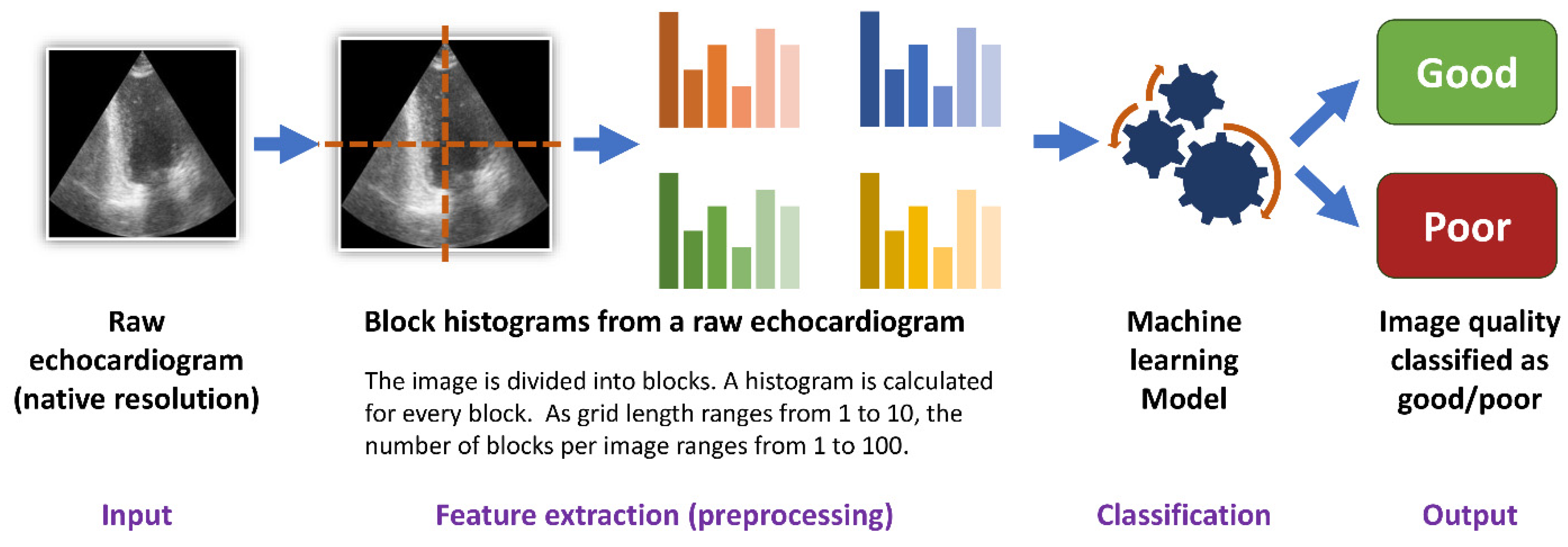
2.5. Histogram Dataset
2.6. Machine Learning
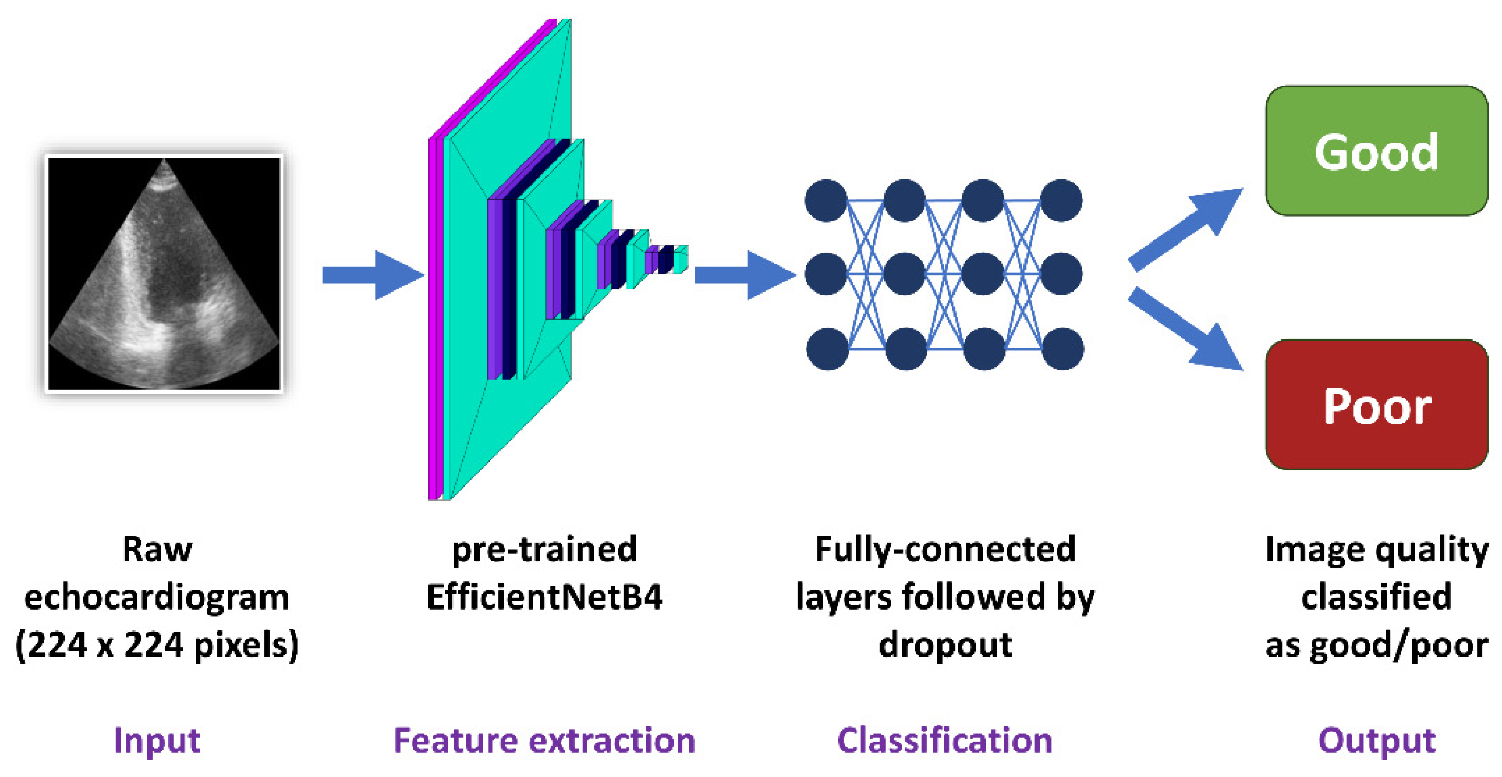
2.7. Deep Learning—Convolutional Neural Networks
2.8. Statistical Analysis
3. Results
3.1. CAMUS Apical 2-Chamber View
3.2. CAMUS Apical 4-Chamber View
3.3. Unity Imaging Parasternal Long-Axis View
3.4. Unity Imaging Apical 4-Chamber View
3.5. Trends in Predictions
3.6. Open-Source Availability of the Best Models
4. Discussion
4.1. Accuracy of Predictions
4.2. Block Histograms: A Novel Approach for Image Quality Analysis
4.3. Factors Determining the Accuracy of the Models
4.4. Sensitivity and Specificity of the Algorithms
4.5. Comparison with Other Studies
5. Limitations
6. Conclusions
Supplementary Materials
Author Contributions
Funding
Institutional Review Board Statement
Informed Consent Statement
Data Availability Statement
Conflicts of Interest
References
- Nagata, Y.; Kado, Y.; Onoue, T.; Otani, K.; Nakazono, A.; Otsuji, Y.; Takeuchi, M. Impact of Image Quality on Reliability of the Measurements of Left Ventricular Systolic Function and Global Longitudinal Strain in 2D Echocardiography. Echo Res. Pract. 2018, 5, 27–39. [Google Scholar] [CrossRef]
- Huang, K.C.; Huang, C.S.; Su, M.Y.; Hung, C.L.; Ethan Tu, Y.C.; Lin, L.C.; Hwang, J.J. Artificial Intelligence Aids Cardiac Image Quality Assessment for Improving Precision in Strain Measurements. JACC Cardiovasc. Imaging 2021, 14, 335–345. [Google Scholar] [CrossRef]
- Sengupta, P.P.; Marwick, T.H. Enforcing Quality in Strain Imaging Through AI-Powered Surveillance. JACC Cardiovasc. Imaging 2021, 14, 346–349. [Google Scholar] [CrossRef] [PubMed]
- Al Saikhan, L.; Park, C.; Hughes, A.D. Reproducibility of Left Ventricular Dyssynchrony Indices by Three-Dimensional Speckle-Tracking Echocardiography: The Impact of Sub-Optimal Image Quality. Front. Cardiovasc. Med. 2019, 6, 149. [Google Scholar] [CrossRef]
- Johnson, K.W.; Torres Soto, J.; Glicksberg, B.S.; Shameer, K.; Miotto, R.; Ali, M.; Ashley, E.; Dudley, J.T. Artificial Intelligence in Cardiology. J. Am. Coll. Cardiol. 2018, 71, 2668–2679. [Google Scholar] [CrossRef]
- Bizopoulos, P.; Koutsouris, D. Deep Learning in Cardiology. IEEE Rev. Biomed. Eng. 2019, 12, 168–193. [Google Scholar] [CrossRef]
- He, B.; Kwan, A.C.; Cho, J.H.; Yuan, N.; Pollick, C.; Shiota, T.; Ebinger, J.; Bello, N.A.; Wei, J.; Josan, K.; et al. Blinded, Randomized Trial of Sonographer versus AI Cardiac Function Assessment. Nature 2023, 616, 520–524. [Google Scholar] [CrossRef]
- Harjoko, R.P.; Sobirin, M.A.; Uddin, I.; Bahrudin, U.; Maharani, N.; Herminingsih, S.; Tsutsui, H. Trimetazidine Improves Left Ventricular Global Longitudinal Strain Value in Patients with Heart Failure with Reduced Ejection Fraction Due to Ischemic Heart Disease. Drug Discov. Ther. 2022, 16, 177–184. [Google Scholar] [CrossRef] [PubMed]
- Mazzetti, S.; Scifo, C.; Abete, R.; Margonato, D.; Chioffi, M.; Rossi, J.; Pisani, M.; Passafaro, G.; Grillo, M.; Poggio, D.; et al. Short-Term Echocardiographic Evaluation by Global Longitudinal Strain in Patients with Heart Failure Treated with Sacubitril/Valsartan. ESC Heart Fail. 2020, 7, 964–972. [Google Scholar] [CrossRef]
- Sławiński, G.; Hawryszko, M.; Liżewska-Springer, A.; Nabiałek-Trojanowska, I.; Lewicka, E. Global Longitudinal Strain in Cardio-Oncology: A Review. Cancers 2023, 15, 986. [Google Scholar] [CrossRef]
- Ramesh, A.N.; Kambhampati, C.; Monson, J.R.T.; Drew, P.J. Artificial Intelligence in Medicine. Ann. R. Coll. Surg. Engl. 2004, 86, 334–338. [Google Scholar] [CrossRef] [PubMed]
- Galmarini, C.M.; Lucius, M. Artificial Intelligence: A Disruptive Tool for a Smarter Medicine. Eur. Rev. Med. Pharmacol. Sci. 2020, 24, 7462–7474. [Google Scholar] [CrossRef] [PubMed]
- Wagner, M.W.; Namdar, K.; Biswas, A.; Monah, S.; Khalvati, F.; Ertl-Wagner, B.B. Radiomics, Machine Learning, and Artificial Intelligence—What the Neuroradiologist Needs to Know. Neuroradiology 2021, 63, 1957. [Google Scholar] [CrossRef] [PubMed]
- Topol, E.J. High-Performance Medicine: The Convergence of Human and Artificial Intelligence. Nat. Med. 2019, 25, 44–56. [Google Scholar] [CrossRef] [PubMed]
- Howard, J.P.; Stowell, C.C.; Cole, G.D.; Ananthan, K.; Demetrescu, C.D.; Pearce, K.; Rajani, R.; Sehmi, J.; Vimalesvaran, K.; Kanaganayagam, G.S.; et al. Automated Left Ventricular Dimension Assessment Using Artificial Intelligence Developed and Validated by a UK-Wide Collaborative. Circ. Cardiovasc. Imaging 2021, 14, E011951. [Google Scholar] [CrossRef] [PubMed]
- Chao, P.K.; Wang, C.L.; Chan, H.L. An Intelligent Classifier for Prognosis of Cardiac Resynchronization Therapy Based on Speckle-Tracking Echocardiograms. Artif. Intell. Med. 2012, 54, 181–188. [Google Scholar] [CrossRef]
- Dong, J.; Liu, S.; Liao, Y.; Wen, H.; Lei, B.; Li, S.; Wang, T. A Generic Quality Control Framework for Fetal Ultrasound Cardiac Four-Chamber Planes. IEEE J. Biomed. Health Inform. 2020, 24, 931–942. [Google Scholar] [CrossRef] [PubMed]
- Luong, C.; Liao, Z.; Abdi, A.; Girgis, H.; Rohling, R.; Gin, K.; Jue, J.; Yeung, D.; Szefer, E.; Thompson, D.; et al. Automated Estimation of Echocardiogram Image Quality in Hospitalized Patients. Int. J. Cardiovasc. Imaging 2021, 37, 229–239. [Google Scholar] [CrossRef] [PubMed]
- Labs, R.B.; Vrettos, A.; Loo, J.; Zolgharni, M. Automated Assessment of Transthoracic Echocardiogram Image Quality Using Deep Neural Networks. Intell. Med. 2023, 3, 191–199. [Google Scholar] [CrossRef]
- Krizhevsky, A.; Sutskever, I.; Hinton, G.E. ImageNet Classification with Deep Convolutional Neural Networks. In Proceedings of the Advances in Neural Information Processing Systems 25 (NIPS 2012), Lake Tahoe, CA, USA, 3–6 December 2012; pp. 1097–1105. [Google Scholar]
- Tandon, A.; Mohan, N.; Jensen, C.; Burkhardt, B.E.U.; Gooty, V.; Castellanos, D.A.; McKenzie, P.L.; Zahr, R.A.; Bhattaru, A.; Abdulkarim, M.; et al. Retraining Convolutional Neural Networks for Specialized Cardiovascular Imaging Tasks: Lessons from Tetralogy of Fallot. Pediatr. Cardiol. 2021, 42, 578–589. [Google Scholar] [CrossRef]
- Tan, M.; Le, Q.V. EfficientNet: Rethinking Model Scaling for Convolutional Neural Networks. In Proceedings of the 36th International Conference on Machine Learning, Long Beach, CA, USA, 9–15 June 2019. [Google Scholar]
- Cikes, M.; Sanchez-Martinez, S.; Claggett, B.; Duchateau, N.; Piella, G.; Butakoff, C.; Pouleur, A.C.; Knappe, D.; Biering-Sørensen, T.; Kutyifa, V.; et al. Machine Learning-Based Phenogrouping in Heart Failure to Identify Responders to Cardiac Resynchronization Therapy. Eur. J. Heart Fail. 2019, 21, 74–85. [Google Scholar] [CrossRef] [PubMed]
- Howell, S.J.; Stivland, T.; Stein, K.; Ellenbogen, K.A.; Tereshchenko, L.G. Using Machine-Learning for Prediction of the Response to Cardiac Resynchronization Therapy: The SMART-AV Study. JACC Clin. Electrophysiol. 2021, 7, 1505–1515. [Google Scholar] [CrossRef]
- Pietka, E. Image Standardization in PACS. In Handbook of Medical Imaging; Academic Press: Cambridge, MA, USA, 2000; pp. 783–801. [Google Scholar] [CrossRef]
- Leclerc, S.; Smistad, E.; Pedrosa, J.; Ostvik, A.; Cervenansky, F.; Espinosa, F.; Espeland, T.; Berg, E.A.R.; Jodoin, P.M.; Grenier, T.; et al. Deep Learning for Segmentation Using an Open Large-Scale Dataset in 2D Echocardiography. IEEE Trans. Med. Imaging 2019, 38, 2198–2210. [Google Scholar] [CrossRef]
- Sengupta, P.P.; Shrestha, S.; Berthon, B.; Messas, E.; Donal, E.; Tison, G.H.; Min, J.K.; D’hooge, J.; Voigt, J.U.; Dudley, J.; et al. Proposed Requirements for Cardiovascular Imaging-Related Machine Learning Evaluation (PRIME): A Checklist: Reviewed by the American College of Cardiology Healthcare Innovation Council. JACC Cardiovasc. Imaging 2020, 13, 2017–2035. [Google Scholar] [CrossRef] [PubMed]
- Monaghan, T.F.; Rahman, S.N.; Agudelo, C.W.; Wein, A.J.; Lazar, J.M.; Everaert, K.; Dmochowski, R.R. Foundational Statistical Principles in Medical Research: Sensitivity, Specificity, Positive Predictive Value, and Negative Predictive Value. Medicina 2021, 57, 503. [Google Scholar] [CrossRef] [PubMed]
- Sajjadian, M.; Lam, R.W.; Milev, R.; Rotzinger, S.; Frey, B.N.; Soares, C.N.; Parikh, S.V.; Foster, J.A.; Turecki, G.; Müller, D.J.; et al. Machine Learning in the Prediction of Depression Treatment Outcomes: A Systematic Review and Meta-Analysis. Psychol. Med. 2021, 51, 2742–2751. [Google Scholar] [CrossRef]
- Jones, D.S.; Podolsky, S.H. The History and Fate of the Gold Standard. Lancet 2015, 385, 1502–1503. [Google Scholar] [CrossRef]
- Puyol-Antón, E.; Sidhu, B.S.; Gould, J.; Porter, B.; Elliott, M.K.; Mehta, V.; Rinaldi, C.A.; King, A.P. A Multimodal Deep Learning Model for Cardiac Resynchronisation Therapy Response Prediction. Med. Image Anal. 2022, 79, 102465. [Google Scholar] [CrossRef]
- Degerli, A.; Kiranyaz, S.; Hamid, T.; Mazhar, R.; Gabbouj, M. Early Myocardial Infarction Detection over Multi-View Echocardiography. Biomed. Signal Process Control 2024, 87, 105448. [Google Scholar] [CrossRef]
- Nazar, W.; Szymanowicz, S.; Nazar, K.; Kaufmann, D.; Wabich, E.; Braun-Dullaeus, R.; Daniłowicz-Szymanowicz, L. Artificial Intelligence Models in Prediction of Response to Cardiac Resynchronization Therapy: A Systematic Review. Heart Fail. Rev. 2023, 29, 133–150. [Google Scholar] [CrossRef]
- Poon, A.I.F.; Sung, J.J.Y. Opening the Black Box of AI-Medicine. J. Gastroenterol. Hepatol. 2021, 36, 581–584. [Google Scholar] [CrossRef] [PubMed]


| Dataset (View) | Characteristics | Mean | Median | Min | Max | Standard Deviation |
|---|---|---|---|---|---|---|
| CAMUS (apical 2-chamber) | image height in pixels | 984.0 | 973.0 | 584.0 | 1945.0 | 157.8 |
| image width in pixels | 600.9 | 591.0 | 323.0 | 1181.0 | 104.5 | |
| mean brightness | 50.2 | 49.3 | 14.8 | 104.0 | 12.2 | |
| number of pixels | 606,740.2 | 575,043.0 | 206,736.0 | 229,7045.0 | 202,752.9 | |
| width-to-height ratio | 0.6 | 0.6 | 0.5 | 0.9 | 0.0 | |
| CAMUS (apical 4-chamber) | image height in pixels | 985.2 | 973.0 | 584.0 | 1945.0 | 160.8 |
| image width in pixels | 599.4 | 591.0 | 323.0 | 1181.0 | 105.6 | |
| mean brightness | 50.5 | 49.8 | 20.0 | 95.0 | 11.8 | |
| number of pixels | 606,721.2 | 575,043.0 | 206,736.0 | 229,7045.0 | 205,842.2 | |
| width-to-height ratio | 0.6 | 0.6 | 0.5 | 0.9 | 0.0 | |
| Unity Imaging (parasternal long-axis) | image height in pixels | 554.7 | 600.0 | 300.0 | 768.0 | 81.1 |
| image width in pixels | 749.3 | 800.0 | 400.0 | 1024.0 | 95.7 | |
| mean brightness | 17.6 | 17.0 | 3.7 | 42.1 | 6.5 | |
| number of pixels | 423,200.0 | 480,000.0 | 120,000.0 | 786,432.0 | 110,102.8 | |
| width-to-height ratio | 1.4 | 1.3 | 1.3 | 1.5 | 0.1 | |
| Unity Imaging (apical 4-chamber) | image height in pixels | 548.0 | 600.0 | 300.0 | 768.0 | 101.2 |
| image width in pixels | 754.4 | 800.0 | 400.0 | 1024.0 | 108.9 | |
| mean brightness | 18.7 | 17.4 | 5.2 | 71.4 | 7.7 | |
| number of pixels | 424,257.0 | 480,000.0 | 120,000.0 | 786,432.0 | 140,175.5 | |
| width-to-height ratio | 1.4 | 1.3 | 1.3 | 1.5 | 0.1 |
| Dataset—Best Model (Grid Length) | Evaluation Metrics | Fold during 5-Fold Cross-Validation | Average | Standard Deviation | ||||
|---|---|---|---|---|---|---|---|---|
| 1 | 2 | 3 | 4 | 5 | ||||
| CAMUS apical 2-chamber view—Random Forest classifier (grid length 5) | Accuracy | 0.72 | 0.79 | 0.79 | 0.71 | 0.78 | 0.76 | 0.04 |
| Sensitivity | 0.68 | 0.70 | 0.70 | 0.63 | 0.70 | 0.68 | 0.03 | |
| Specificity | 0.75 | 0.86 | 0.86 | 0.77 | 0.84 | 0.82 | 0.05 | |
| AUC | 0.80 | 0.86 | 0.83 | 0.78 | 0.83 | 0.82 | 0.03 | |
| True negative | 42 | 48 | 49 | 44 | 48 | 46.20 | 3.03 | |
| False positive | 14 | 8 | 8 | 13 | 9 | 10.40 | 2.88 | |
| False negative | 14 | 13 | 13 | 16 | 13 | 13.80 | 1.30 | |
| True positive | 30 | 31 | 30 | 27 | 30 | 29.60 | 1.52 | |
| CAMUS apical 4-chamber view—Random Forest classifier (grid length 10) | Accuracy | 0.71 | 0.80 | 0.71 | 0.78 | 0.72 | 0.74 | 0.04 |
| Sensitivity | 0.70 | 0.82 | 0.81 | 0.86 | 0.84 | 0.81 | 0.06 | |
| Specificity | 0.72 | 0.77 | 0.57 | 0.67 | 0.55 | 0.65 | 0.09 | |
| AUC | 0.77 | 0.86 | 0.78 | 0.83 | 0.78 | 0.81 | 0.04 | |
| True negative | 31 | 33 | 24 | 28 | 23 | 27.80 | 4.32 | |
| False positive | 12 | 10 | 18 | 14 | 19 | 14.60 | 3.85 | |
| False negative | 17 | 10 | 11 | 8 | 9 | 11.00 | 3.54 | |
| True positive | 40 | 47 | 47 | 50 | 49 | 46.60 | 3.91 | |
| Unity Imaging parasternal long-axis view—XGBoost classifier (grid length 10) | Accuracy | 0.80 | 0.81 | 0.84 | 0.85 | 0.83 | 0.83 | 0.02 |
| Sensitivity | 0.53 | 0.57 | 0.63 | 0.67 | 0.64 | 0.61 | 0.06 | |
| Specificity | 0.94 | 0.94 | 0.95 | 0.95 | 0.93 | 0.94 | 0.01 | |
| AUC | 0.85 | 0.86 | 0.89 | 0.91 | 0.86 | 0.88 | 0.03 | |
| True negative | 189 | 189 | 190 | 189 | 185 | 188.40 | 1.95 | |
| False positive | 12 | 12 | 10 | 11 | 15 | 12.00 | 1.87 | |
| False negative | 50 | 45 | 39 | 35 | 38 | 41.40 | 6.02 | |
| True positive | 56 | 60 | 67 | 71 | 68 | 64.40 | 6.19 | |
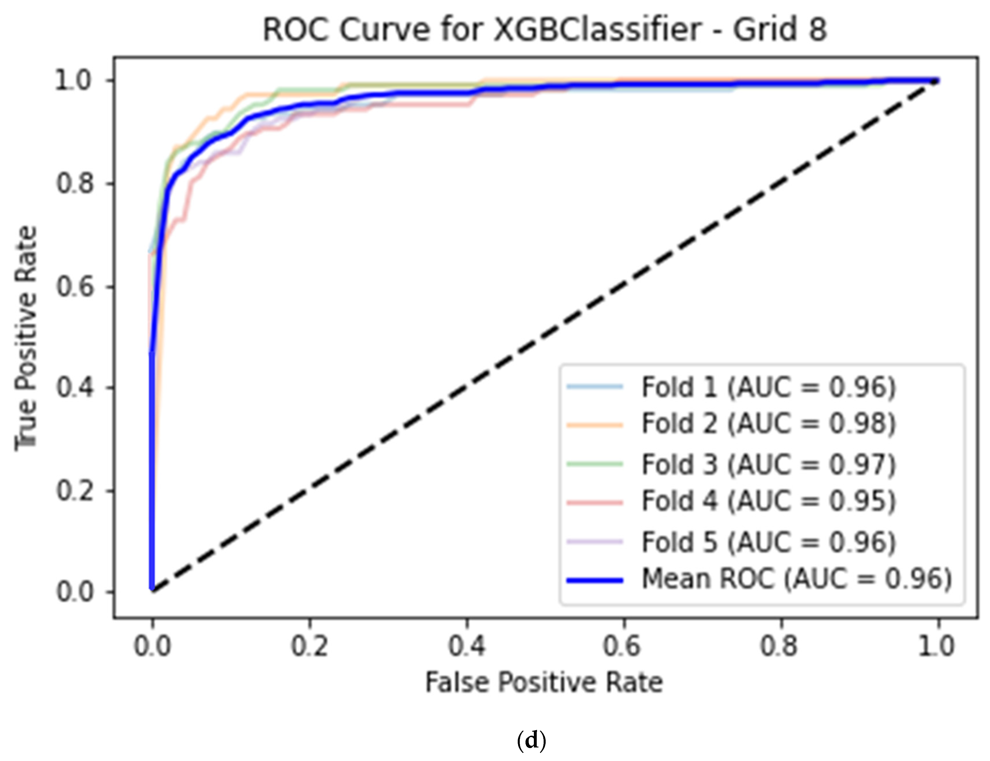
| Unity Imaging apical 4-chamber view—XGBoost classifier (grid length 8) | Accuracy | 0.92 | 0.93 | 0.92 | 0.90 | 0.91 | 0.92 | 0.01 |
| Sensitivity | 0.79 | 0.88 | 0.80 | 0.80 | 0.82 | 0.82 | 0.03 | |
| Specificity | 0.98 | 0.96 | 0.99 | 0.95 | 0.96 | 0.97 | 0.02 | |
| AUC | 0.96 | 0.98 | 0.97 | 0.95 | 0.96 | 0.96 | 0.01 | |
| True negative | 201 | 196 | 203 | 196 | 197 | 198.60 | 3.21 | |
| False positive | 4 | 9 | 3 | 10 | 8 | 6.80 | 3.11 | |
| False negative | 22 | 13 | 21 | 21 | 19 | 19.20 | 3.63 | |
| True positive | 85 | 94 | 85 | 85 | 87 | 87.20 | 3.90 | |
| Dataset | Evaluation Metrics | Fold during 5-Fold Cross-Validation | Average | Standard Deviation | ||||
|---|---|---|---|---|---|---|---|---|
| 1 | 2 | 3 | 4 | 5 | ||||
| CAMUS apical 2-chamber view | Accuracy | 0.72 | 0.80 | 0.72 | 0.79 | 0.76 | 0.76 | 0.04 |
| Sensitivity | 0.49 | 0.77 | 0.58 | 0.64 | 0.70 | 0.64 | 0.11 | |
| Specificity | 0.89 | 0.82 | 0.82 | 0.91 | 0.80 | 0.85 | 0.05 | |
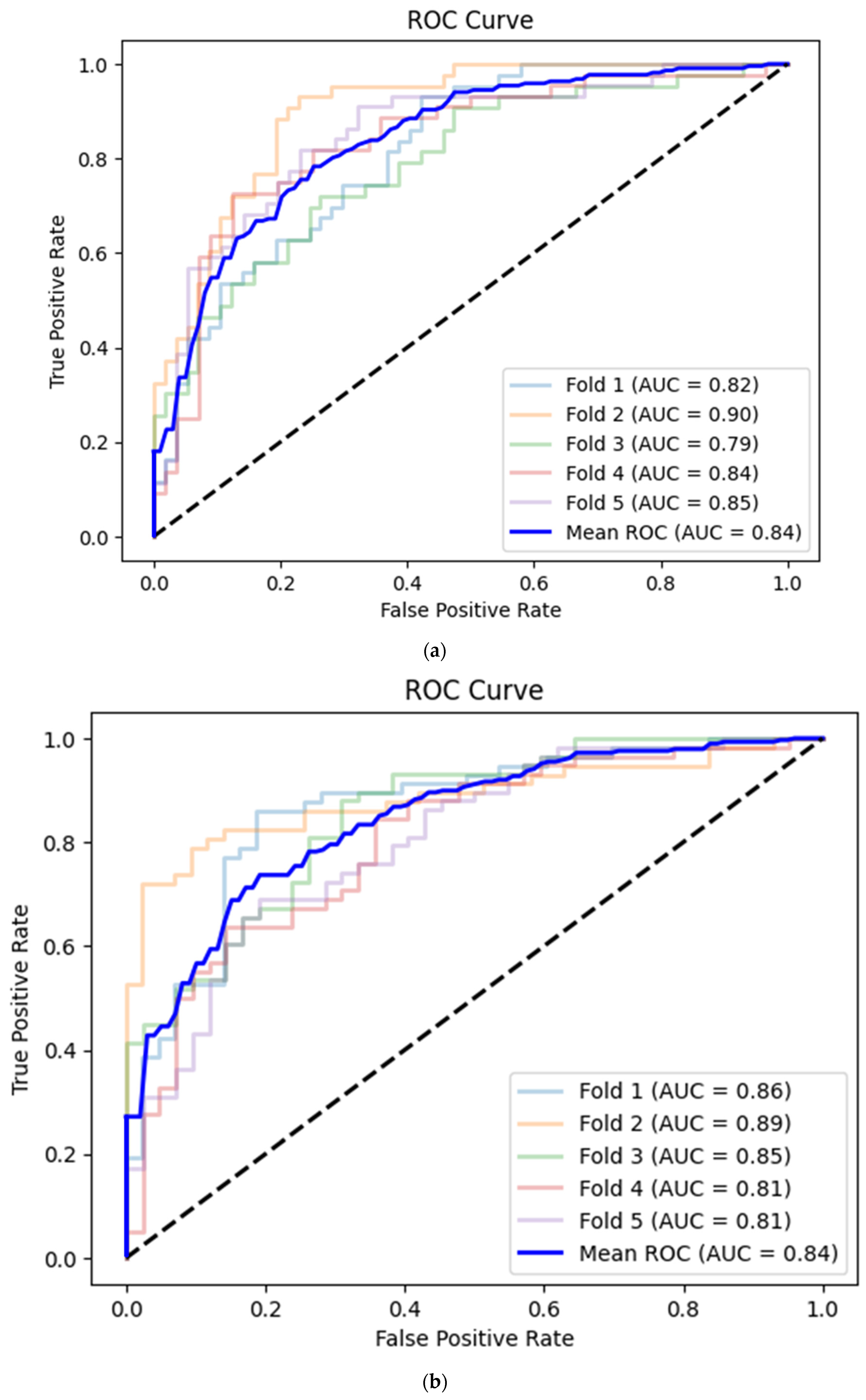
| AUC | 0.82 | 0.90 | 0.79 | 0.84 | 0.85 | 0.84 | 0.04 | |
| True negative | 51 | 47 | 47 | 51 | 45 | 48.20 | 2.68 | |
| False positive | 6 | 10 | 10 | 5 | 11 | 8.40 | 2.70 | |
| False negative | 22 | 10 | 18 | 16 | 13 | 15.80 | 4.60 | |
| True positive | 21 | 33 | 25 | 28 | 31 | 27.60 | 4.77 | |
| CAMUS apical 4-chamber view | Accuracy | 0.82 | 0.69 | 0.74 | 0.76 | 0.71 | 0.74 | 0.05 |
| Sensitivity | 0.89 | 0.95 | 0.74 | 0.84 | 0.71 | 0.83 | 0.10 | |
| Specificity | 0.72 | 0.35 | 0.74 | 0.64 | 0.71 | 0.63 | 0.16 | |
| AUC | 0.86 | 0.89 | 0.85 | 0.81 | 0.81 | 0.84 | 0.04 | |
| True negative | 31 | 15 | 31 | 27 | 30 | 26.80 | 6.80 | |
| False positive | 12 | 28 | 11 | 15 | 12 | 15.60 | 7.09 | |
| False negative | 6 | 3 | 15 | 9 | 17 | 10.00 | 5.92 | |
| True positive | 51 | 54 | 43 | 49 | 41 | 47.60 | 5.46 | |
| Unity Imaging parasternal long-axis view | Accuracy | 0.78 | 0.75 | 0.76 | 0.75 | 0.72 | 0.75 | 0.02 |
| Sensitivity | 0.71 | 0.35 | 0.55 | 0.53 | 0.60 | 0.55 | 0.13 | |
| Specificity | 0.81 | 0.97 | 0.88 | 0.88 | 0.78 | 0.86 | 0.07 | |
| AUC | 0.83 | 0.81 | 0.80 | 0.75 | 0.77 | 0.79 | 0.03 | |
| True negative | 163 | 194 | 175 | 175 | 156 | 172.60 | 14.47 | |
| False positive | 38 | 6 | 25 | 25 | 45 | 27.80 | 14.92 | |
| False negative | 31 | 69 | 48 | 50 | 42 | 48.00 | 13.87 | |
| True positive | 75 | 37 | 58 | 56 | 63 | 57.80 | 13.77 | |
| Unity Imaging apical 4-chamber view | Accuracy | 0.88 | 0.88 | 0.89 | 0.89 | 0.89 | 0.89 | 0.01 |
| Sensitivity | 0.79 | 0.68 | 0.78 | 0.86 | 0.84 | 0.79 | 0.07 | |
| Specificity | 0.93 | 0.98 | 0.95 | 0.91 | 0.92 | 0.94 | 0.03 | |
| AUC | 0.94 | 0.96 | 0.95 | 0.95 | 0.97 | 0.95 | 0.01 | |
| True negative | 190 | 201 | 195 | 188 | 189 | 192.60 | 5.41 | |
| False positive | 15 | 4 | 11 | 18 | 16 | 12.80 | 5.54 | |
| False negative | 22 | 34 | 23 | 15 | 17 | 22.20 | 7.40 | |
| True positive | 85 | 73 | 83 | 91 | 89 | 84.20 | 7.01 | |
| Dataset and Best Models | Evaluation Metrics | CNN (Deep Learning) | Machine Learning | p-Value |
|---|---|---|---|---|
| CAMUS apical 2-chamber view: CNN versus Random Forest classifier (grid length 5) | Accuracy | 0.76 (95% CI 0.72–0.79) | 0.76 (95% CI 0.72–0.79) | 1.000 |
| Sensitivity | 0.64 (95% CI 0.59–0.68) | 0.68 (95% CI 0.64–0.72) | 0.140 | |
| Specificity | 0.85 (95% CI 0.82–0.88) | 0.82 (95% CI 0.78–0.85) | 0.155 | |
| AUC | 0.84 (95% CI 0.81–0.87) | 0.82 (95% CI 0.78–0.85) | 0.406 | |
| CAMUS apical 4-chamber view: CNN versus Random Forest classifier (grid length 10) | Accuracy | 0.74 (95% CI 0.70–0.78) | 0.74 (95% CI 0.70–0.78) | 1.000 |
| Sensitivity | 0.83 (95% CI 0.79–0.86) | 0.81 (95% CI 0.77–0.84) | 0.503 | |
| Specificity | 0.63 (95% CI 0.59–0.67) | 0.65 (95% CI 0.61–0.70) | 0.513 | |
| AUC | 0.84 (95% CI 0.81–0.87) | 0.81 (95% CI 0.77–0.84) | 0.138 | |
| Unity Imaging parasternal long-axis view: CNN versus XGBoost classifier (grid length 10) | Accuracy | 0.75 (95% CI 0.73–0.77) | 0.83 (95% CI 0.81–0.84) | <0.001 |
| Sensitivity | 0.55 (95% CI 0.52–0.57) | 0.61 (95% CI 0.58–0.63) | <0.001 | |
| Specificity | 0.86 (95% CI 0.84–0.88) | 0.94 (95% CI 0.93–0.95) | <0.001 | |
| AUC | 0.79 (95% CI 0.77–0.81) | 0.88 (95% CI 0.86–0.89) | <0.001 | |
| Unity Imaging apical 4-chamber view: CNN versus XGBoost classifier (grid length 8) | Accuracy | 0.89 (95% CI 0.87–0.90) | 0.92 (95% CI 0.90–0.93) | 0.008 |
| Sensitivity | 0.79 (95% CI 0.77–0.81) | 0.82 (95% CI 0.80–0.84) | 0.054 | |
| Specificity | 0.94 (95% CI 0.92–0.95) | 0.97 (95% CI 0.96–0.97) | <0.001 | |
| AUC | 0.95 (95% CI 0.94–0.96) | 0.96 (95% CI 0.95–0.97) | 0.172 |
Disclaimer/Publisher’s Note: The statements, opinions and data contained in all publications are solely those of the individual author(s) and contributor(s) and not of MDPI and/or the editor(s). MDPI and/or the editor(s) disclaim responsibility for any injury to people or property resulting from any ideas, methods, instructions or products referred to in the content. |
© 2024 by the authors. Licensee MDPI, Basel, Switzerland. This article is an open access article distributed under the terms and conditions of the Creative Commons Attribution (CC BY) license (https://creativecommons.org/licenses/by/4.0/).
Share and Cite
Nazar, W.; Nazar, K.; Daniłowicz-Szymanowicz, L. Machine Learning and Deep Learning Methods for Fast and Accurate Assessment of Transthoracic Echocardiogram Image Quality. Life 2024, 14, 761. https://doi.org/10.3390/life14060761
Nazar W, Nazar K, Daniłowicz-Szymanowicz L. Machine Learning and Deep Learning Methods for Fast and Accurate Assessment of Transthoracic Echocardiogram Image Quality. Life. 2024; 14(6):761. https://doi.org/10.3390/life14060761
Chicago/Turabian StyleNazar, Wojciech, Krzysztof Nazar, and Ludmiła Daniłowicz-Szymanowicz. 2024. "Machine Learning and Deep Learning Methods for Fast and Accurate Assessment of Transthoracic Echocardiogram Image Quality" Life 14, no. 6: 761. https://doi.org/10.3390/life14060761
APA StyleNazar, W., Nazar, K., & Daniłowicz-Szymanowicz, L. (2024). Machine Learning and Deep Learning Methods for Fast and Accurate Assessment of Transthoracic Echocardiogram Image Quality. Life, 14(6), 761. https://doi.org/10.3390/life14060761