Fault Diagnosis of Gearbox Bearings Based on Multi-Feature Fusion Dual-Channel CNN-Transformer-CAM

Abstract

As a core component of the gearbox, bearings are crucial to the stability and reliability of the transmission system. However, dynamic variations in operating conditions and complex noise interference present limitations for existing fault diagnosis methods in processing non-stationary signals and capturing complex features. To address the aforementioned challenges, this paper proposes a bearing fault diagnosis method based on a multi-feature fusion dual-channel CNN-Transformer-CAM framework. The model cross-fuses the two-dimensional feature images from Gramian Angular Difference Field (GADF) and Generalized S Transform (GST), preserving complete time–frequency domain information. First, a dual-channel parallel convolutional structure is employed to separately sample the generalized S-transform (GST) maps and the Gramian Angular Difference Field (GADF) maps, enriching fault information from different dimensions and effectively enhancing the model’s feature extraction capability. Subsequently, a Transformer structure is introduced at the backend of the convolutional neural network to strengthen the representation and analysis of complex time–frequency features. Finally, a cross-attention mechanism is applied to dynamically adjust features from the two channels, achieving adaptive weighted fusion. Test results demonstrate that under conditions of noise interference, limited samples, and multiple operating states, the proposed method can effectively achieve the accurate assessment of bearing fault conditions.

1. Introduction

In recent years, research on the fault diagnosis of rotating machinery has gained significant attention, primarily aiming to prevent equipment damage and unexpected shutdowns [1]. Bearings are critical components of rotating machinery and are widely utilized in fields such as automotive, wind turbines, and aerospace. As key elements in gearbox transmission systems, bearings also represent one of the primary sources of gearbox failures. Therefore, research on fault diagnosis for gearbox bearings is of significant importance [2,3,4].

Numerous scholars have conducted extensive research on the fault diagnosis of gearbox bearings. Some scholars have considered the vibration characteristics of bearing signals and used a combination of time–frequency domain feature extraction and machine learning methods to assess bearing faults based on the original vibration signals. Guo, Z et al. [5] introduced a model integrating wavelet packet transform (WPT) and random forest (RF), which significantly enhanced both the efficiency and classification accuracy of fault diagnosis. Bie, F et al. [6] developed a method that integrates an improved Complete Ensemble Empirical Mode Decomposition with Adaptive Noise (CEEMDAN) algorithm with a Long Short-Term Memory (LSTM) deep neural network. This approach effectively extracts fault features from reciprocating pump vibration signals and achieves accurate classification. He, S et al. [7] developed a fault diagnosis approach based on relevance vector machines (RVMs) tailored for small-sample data, demonstrating considerable potential in fault prediction. Zheng, J et al. [8] introduced a novel approach for rolling bearing fault diagnosis, which utilizes composite multiscale fuzzy entropy (CMFE) and ensemble support vector machines (ESVMs). Li, H et al. [9] developed a parameter-optimized VMD-based diagnostic framework for bearing composite faults, where fault-related components distribute across distinct frequency bands without relying on additional methods. Yang, J et al. [10] developed a fault feature extraction method based on variational mode decomposition (VMD) integration, optimized via IGOOSE and RobustICA-CYCBD, which significantly mitigates the adverse effects of noise in bearing fault signal analysis. Yuan, B et al. [11] proposed an algorithm to optimize VMD and combined it with a CNN-BiLSTM-based fault diagnosis method. This algorithm demonstrates significant advantages in enhancing diagnostic accuracy and generalization capabilities while exhibiting excellent adaptability and robustness.

However, due to the limitations of the methods used in the above studies, the learning depth is insufficient and the interference resistance is poor, making it impossible to identify and evaluate bearing faults at a deeper level. Another group of scholars used deep learning models to solve the problem of fault pattern recognition in bearings. Compared with traditional machine learning algorithms, deep learning models can learn and extract deep features from massive amounts of raw data, significantly improving recognition accuracy and network model computation time, and can effectively identify and evaluate abnormal patterns in bearings under complex operating conditions. Ye, M et al. [12] developed a multi-sensor residual convolutional fusion network (MRCFN) for intelligent bearing fault diagnosis, which overcomes the limitation of incomplete and insufficient fault information from individual sensors. Zhang, W et al. [13] constructed an end-to-end model for bearing fault recognition and evaluation using a one-dimensional convolutional neural network (CNN), which significantly improves the efficiency of bearing fault diagnosis. Zhang, Z et al. [14] developed an intelligent fault diagnosis model for bearings based on dual-level data fusion (DLDF), which achieved reliable diagnostic performance under time-varying rotational speed conditions. To enhance the feature extraction capabilities of deep learning models, attention mechanisms and multi-scale approaches have been incorporated into the models. Zhang, S et al. [15] introduced a selective kernel convolutional deep residual network that incorporates channel–space attention mechanisms and feature fusion. The model embeds a specially designed channel–space attention enhancement module into the selective kernel convolutional deep residual architecture and leverages multi-layer feature fusion for fault diagnosis. Yao, Q et al. [16] developed an improved DDA model utilizing multi-scale domain adaptation (MSDA), which overcomes the limitations of traditional DDA models that are confined to fixed-scale transfer feature (TF) outputs and may lose critical information during domain mixing. To enrich the information of input features, converting one-dimensional time-domain signals into images is also a highly useful technique in fault diagnosis. Spirto, M et al. [17] proposed an SDP-CNN-based fault detection method that significantly reduced the computational time while maintaining equivalent accuracy. Wang, S. and Zhang, J. [18] proposed an intelligent fault diagnosis system that integrated Andrews diagrams with convolutional neural network (CNN) technology, demonstrating significantly better performance compared to traditional neural network-based diagnostic systems. Zhang, Q. and Deng, L. [19] introduced an intelligent fault diagnosis method for rolling bearings that combined short-time Fourier transform with convolutional neural networks (STFT-CNN), effectively mitigating the inherent loss of feature information during the extraction process from raw vibration signals. More recently, the emergence of Large Language Models (LLMs) has introduced a paradigm shift towards knowledge-aware and interactive diagnostic frameworks. By leveraging massive pre-trained knowledge and instruction-following capabilities, LLMs offer the potential to integrate multimodal information. Peng, C. et al. [20] introduced the first large language model (LLM)-based fault diagnosis model for railway vehicle on-board controllers (VOBCs), named RFD-LLM, which enables efficient and accurate identification of seven types of VOBC fault modes. Wang, Z. et al. [21] proposed an industrial large model (CNC-VLM) optimized with reinforcement learning from human feedback (RLHF), which utilizes visual-linguistic multimodal knowledge to achieve autonomous fault detection.

Most existing diagnostic models rely on single feature extraction methods, neglecting the synergistic fusion of time-domain and frequency-domain multimodal information. They lack comprehensive utilization of multiple features, thereby limiting diagnostic performance. Additionally, these methods have limited capability in capturing nonlinear features, making it difficult to address complex failure modes. By comprehensively considering the aforementioned methods, this paper proposes a multi-feature fusion dual-channel CNN-Transformer-CAM method for bearing fault diagnosis. Time–frequency images are generated using the Gramian Angular Difference Field (GADF) and the Generalized S Transform (GST), thereby overcoming the limitations of traditional methods in processing non-stationary signals and capturing complex features. These feature maps are subsequently processed through dual-channel parallel convolutions. Parallel convolutions enable simultaneous processing of multiple feature maps, effectively enhancing the model’s feature extraction capability and facilitating the capture of multi-scale features within the signal. Additionally, a Transformer Encoder architecture is introduced at the backend of each CNN. Transformer models excel at capturing long-range dependencies and complex global features, while CNNs excel at local feature extraction. Combining both enhances the model’s overall performance, strengthening its ability to express and analyze complex spatiotemporal features. Finally, a cross-attention mechanism dynamically adjusts features across the two channels, enabling the adaptive weighted fusion of features.

The contributions of this study can be summarized as follows:

1. A dual-channel CNN-Transformer-CAM fault diagnosis model featuring multi-feature deep fusion is proposed. By cross-fusing two-dimensional feature images generated from Gramian Angle Difference Field (GADF) and generalized S-transform (GST), this model effectively preserves the complete information in both the time domain and time–frequency domain of vibration signals. It overcomes the limitations of traditional methods when handling non-stationary signals and complex features.

2. A feature extraction architecture combining dual-channel parallel convolution and Transformer is designed. The two channels separately process Gramian Angle Difference Field (GADF) and generalized S-transform (GST) feature maps, which enhances the model’s ability to extract multi-scale and multi-dimensional fault features. A Transformer encoder is further introduced at the backend of the CNN, strengthening the model’s capacity to model long-range dependencies within complex time–frequency characteristics.

3. A cross-attention mechanism (CAM) is introduced to achieve adaptive fusion of features. During the dual-channel feature fusion stage, CAM dynamically calculates and adjusts the weights, enabling more effective weighted fusion of features. This enhancement improves the model’s ability to focus on critical fault features and increases classification accuracy.

4. The model’s performance was validated. Experiments demonstrated that this method maintains high diagnostic accuracy and stability under conditions of noise interference, sparse data, and multiple operating scenarios.

The structure of this paper is as follows. Section 2 outlines the theoretical foundation of the employed methods. Section 3 presents the proposed fault diagnosis methodology. Section 4 provides an analysis of the experimental results and model performance. Finally, Section 5 concludes the research.

2. Fundamental Theory

2.1. Gramian Angle Difference Fields

The Gramian Angular Field (GAF) [22] is a novel encoding technique that transforms one-dimensional time series signals into two-dimensional feature image representations, establishing a connection between conventional time series analysis and deep learning approaches. Central to this method is the use of polar coordinate transformation to map temporal characteristics of the series into the angular domain, followed by the construction of a Gram matrix to preserve temporal dependencies. Two primary variants of GAF are the Gramian Angular Sum Field (GASF) and the Gramian Angular Difference Field (GADF) [23]. Each element of GASF is the cosine value of the angle sum, while each element of GADF is the sine value of the angle difference. Compared to GASF, GADF is more stable when performing two-dimensional feature map conversion. The two-dimensional GADF image is generated by computing the Gram matrix, with the primary formula expressed as follows:

$$\begin{array}{c}{\mathit{G}}_{GADF}=\left[\begin{array}{ccc}\sin ({\varphi }_1-{\varphi }_1)& \cdot \cdot \cdot & \sin ({\varphi }_1-{\varphi }_M)\\ \sin ({\varphi }_2-{\varphi }_1)& \cdot \cdot \cdot & \sin ({\varphi }_2-{\varphi }_M)\\ ⋮& \cdot \cdot \cdot & ⋮\\ \sin ({\varphi }_M-{\varphi }_1)& \cdot \cdot \cdot & \sin ({\varphi }_M-{\varphi }_M)\end{array}\right]\\ =\sqrt{\mathit{I}-{({\tilde{\mathit{X}}}^{\prime T})}^2}\times {\tilde{\mathit{X}}}^{\prime }-{\tilde{\mathit{X}}}^{\prime T}\times \sqrt{\mathit{I}-{\tilde{\mathit{X}}}^{\prime 2}}\end{array}$$

(1)

In the formula, $\mathit{I}$ is the unit vector, and ${\tilde{\mathit{X}}}^{\prime T}$ is the transpose vector of $\widetilde{{\mathit{X}}^{\prime }}$.

Through the above transformation, it can be seen that GAF images can better explain and present the commonalities and potential relationships of vibration signals [24]. The conversion process is shown in Figure 1.

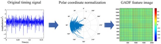
Figure 1. The conversion process of GADF.

2.2. S-Transform

The S-transform (ST) is a time–frequency feature extraction method proposed by Stockwell et al. [25], which combines the advantages of both WT and STFT. Its core lies in the introduction of a Gaussian window function, which allows for dynamic adjustment of time–frequency resolution while preserving phase information, thereby enabling variable time–frequency resolution. Although ST has many advantages in time–frequency analysis, its time–frequency resolution is constrained by the fixed nature of the window function form, which has certain limitations in practical applications. Therefore, GST [26] was developed based on ST. By changing the shape of the Gaussian window function through a given adjustment parameter k, the time–frequency resolution can be improved. The GST formula is:

$${\mathit{S}}^{\prime }(\mathit{\tau },f)={\displaystyle \underset{-\infty }{\overset{+\infty }{\int }}x(t)\frac{\left|\eta f\right|}{\sqrt{2\pi }}}{e}^{-{\displaystyle \frac{{(\tau -t)}^2{\eta }^2{f}^2}{2}}}\cdot e^{-i2\pi ft}dt$$

(2)

By introducing the adjustment parameter $\eta$, the time–frequency resolution of ST can be flexibly adjusted. Figure 2 shows the time–frequency image of a faulty bearing using GST.

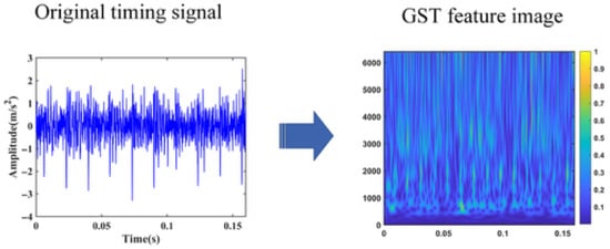
Figure 2. The conversion process of GST.

2.3. Convolutional Neural Network

As a representative deep learning architecture, Convolutional Neural Networks (CNNs) [27] exhibit notable strengths in applications such as bearing fault diagnosis. Typically comprising convolutional layers, pooling layers, activation functions, and fully connected layers, CNNs enable efficient feature extraction and classification. The structure is shown in Figure 3. The convolutional layer employs a predefined-size convolution kernel that slides across the input feature map to perform computations, enabling weighted extraction of local features. The corresponding convolution calculation formula is:

$$x_j^l=f({\displaystyle \sum _{i=1}^M{k}_{ij}^l{x}_i^{l-1}+b_j^l})$$

(3)

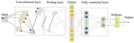
Figure 3. Convolutional neural network model.

In the equation, $x_j^l$ is the jth feature map number in the lth layer, $k_{ij}^l$ is the convolution kernel in the lth layer, and $b_j^l$ is the bias in the lth layer.

The features extracted via convolution are subsequently subjected to downsampling through pooling layers, which further reduces their dimensionality. Commonly used pooling techniques include average pooling and max pooling; in this study, max pooling was adopted for downsampling. To expedite model convergence, batch normalization (BN) is incorporated between the convolutional and pooling layers. The operation of the pooling layer can be formally expressed as follows:

$$p_i^l(j)=\max \{q_i^l(t)\},(j-1)W^{\prime }+1\le t\le j{W}^{\prime }$$

(4)

In the equation, $p_i^l(j)$ is the output value of the pooling layer, $q_i^l(t)$ is the activation value of the tth neuron in the ith feature of the lth layer, and $W^{\prime }$ is the width of the convolution kernel.

Finally, a fully connected layer integrates high-level features to form the basis for classification, which is then performed using the Softmax function.

2.4. Transformers and Attention Mechanisms

The Transformer architecture [28] diverges markedly from convolutional neural networks (CNNs). As a neural network model built upon the attention mechanism, it is fundamentally structured with two key components: an encoder and a decoder. The encoder learns feature representations from the input signal and forwards the extracted features to the decoder. Upon receiving these features, the decoder generates predictions and ultimately outputs the result with the highest probability. Central to this model is the Multi-head Self-Attention (MSA) mechanism [29]. This mechanism employs multiple Scaled Dot-Product Attention (SDA) modules to split the input signal into separate sets of Query (Q), Key (K), and Value (V) matrices. These matrices are then projected into distinct subspaces and processed in parallel by independent attention heads.

MSA consists of several independent self-attention modules. The self-attention mechanism computes attention weights by evaluating the inner products among queries, keys, and values, followed by a weighted summation of the values to produce the final output. The corresponding calculation is given as follows.

$$\left\{\begin{array}{c}Attention\left(Q,K,V\right)=Soft\max \left(Q{K}^T/\sqrt{d_k}\right)V\\ Q=X{W}_Q\\ K=X{W}_K\\ V=X{W}_V\end{array}\right.$$

(5)

In the formula, Q is the query matrix; K is the key matrix; V is the value matrix; $W_Q$, $W_K$, and $W_V$ are the corresponding weight matrices for Q, K, and V, respectively.

As shown in Figure 4, each head is concatenated using Concat, and the result is multiplied by the weight matrix $W^o$. The multi-head self-attention output is as follows:

$$\left\{\begin{array}{c}MultiHead(Q,K,V)=Concat(hea{d}_1,hea{d}_2,\dots ,hea{d}_h)W^o\\ hea{d}_i=Att(Q{W}_i^Q,K{W}_i^K,V{W}_i^V)\end{array}\right.$$

(6)

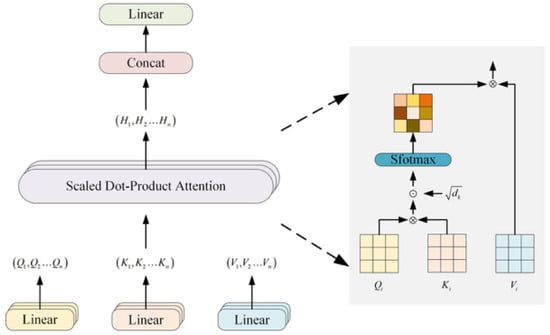
Figure 4. Multi-head Attention Mechanism.

In the equation, Concat concatenates the outputs of multiple attention heads. $W_i^Q$, $W_i^K$, and $W_i^V$ represent the weight matrices of the i-th attention head, where i ranges from $i\in (1,h)$.

3. The Proposed Method

3.1. Model Structure

The model structure of this paper is shown in Figure 5. First, the collected one-dimensional time-domain signals are segmented. Specifically, an overlapping sampling approach is adopted with a window length of 2048 and an overlap ratio of 50% for sliding segmentation. Subsequently, GADF and GST transforms are applied to these segmented signal units to generate their corresponding feature representations. During the feature extraction stage, the one-dimensional vibration signal of rolling bearings exhibits limited representational information. Directly employing a single convolutional neural network can only extract local features of the signal, resulting in limited extraction effectiveness. Therefore, this study explores the hidden feature information within the signal from a multi-feature perspective. By constructing a parallel feature extraction module, two-dimensional GADF time-domain and GST time–frequency feature images are cross-fused. Each branch uses identical convolutional kernels for feature sampling, followed by regularization to enhance the model’s generalization ability. Max pooling is adopted for the pooling operation to retain the most salient features and strengthen texture information. Subsequently, the feature information extracted from the two branches is transformed into one-dimensional vectors through a flattening layer and fed into the Transformer Encoder for further feature encoding and interactive learning. The Transformer Encoder captures long-range dependencies among features and generates more expressive feature representations. After being processed by the Transformer Encoder, the two parallel channels yield two distinct feature vectors. Most commonly adopted multi-scale or multi-channel feature fusion approaches primarily rely on simple concatenation, which often results in redundant fused features that are detrimental to model learning. During the fusion process, this paper treated frequency-domain features as query sequences and time-series features as key–value pair sequences. By calculating attention weights between the query sequence and key–value pair sequence, it models the degree of association between different features. Finally, the feature vectors are fed into a linear layer for the final classification task, thereby outputting the diagnostic results. The processed two-dimensional feature images are input into the model proposed in this paper for multiple training iterations. The model’s key hyperparameters are determined through empirical systematic manual tuning. The main parameters are shown in Table 1.

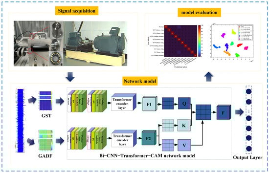
Figure 5. The CNN-Transformer-CAM model framework proposed in this paper.

Table 1. Key parameters of the model.

Name	Kernel Size	Number of Channels/Value
Conv2D_1_1	3 × 3	16
Maxpool_1_1	2 × 2	16
Conv2D_1_2	3 × 3	32
Maxpool_1_2	2 × 2	32
Conv2D_1_3	5 × 5	32
Adaptive Maxpool_1_3	—	32
Transformer_1_d_embed	—	128
Transformer_1_num_heads	—	4
Conv2D_2_1	3 × 3	16
Maxpool_2_1	2 × 2	16
Conv2D_2_2	3 × 3	32
Maxpool_2_2	2 × 2	32
Conv2D_2_3	5 × 5	32
Adaptive Maxpool_2_3	—	32
Transformer_2_d_embed	—	128
Transformer_2_num_heads	—	4
Learning rate	—	0.001
Epoch	—	50
Batch size	—	64

3.2. Model Diagnosis Process

The diagnostic process of the dual-channel parallel CNN-Transformer-CAM model constructed in this paper is illustrated in Figure 6.

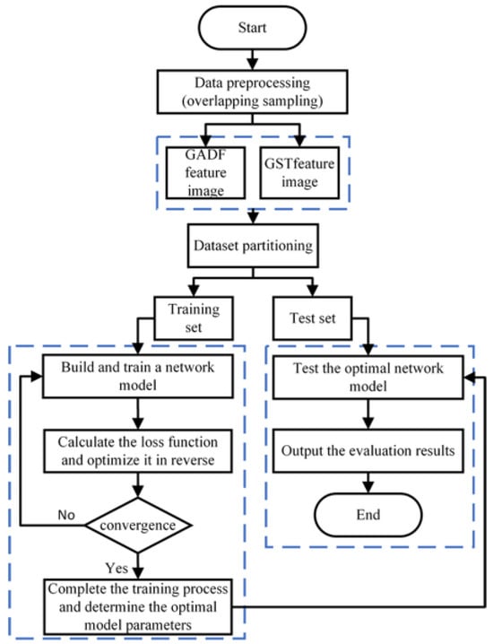
Figure 6. Model evaluation process.

Step 1: Acquire raw vibration signals from the laboratory under different fault conditions for subsequent model training.

Step 2: The original data are segmented into samples using an overlapping sampling method, followed by normalization of the sample data. This paper employed minimum-maximum normalization. Subsequently, the one-dimensional vibration signals are converted into two-dimensional images via Gramian Angular Difference Field transformation and generalized S-transform to serve as input samples, which are then divided into training and testing sets in a ratio of 7:3.

Step 3: Build the CNN-Transformer-CAM network model and initialize the model parameters.

Step 4: Input the partitioned training set into the model for training. If the model converges to the desired outcome, proceed to the next step; otherwise, modify the model parameters until optimal parameters are achieved, then retain the optimal model.

Step 5: The divided test set samples are fed into the optimal model, yielding the final classification results and test accuracy.

4. Test Results and Analysis

4.1. Dataset Description

Vibration signals from bearings with varying degrees of failure are collected via a gearbox bearing failure simulation test bench. As shown in Figure 7, the bearing test bench consists of a motor, parallel gearbox, planetary gearbox, torque measuring instrument, coupling, and magnetic powder brake. The bearing models used were NJ205EM (TMB, Quzhou, China) and NF205EM (TMB). The bearing condition types included four categories: normal, inner ring failure, rolling element failure, and outer ring failure. The fault severity levels were width × depth: 0.3 × 0.2 mm, 0.7 × 0.6 mm, and 1.1 × 1 mm. All faults were machined using an electric discharge machining (EDM) machine. The bearing fault machining test is shown in Figure 8. The data logger model was uT3408M (Manufacturer: uTeKL, Wuhan, China), with a sampling frequency of 12.8 kHz and a sampling time of 10.24 s. This experiment simulated four types of bearing operating conditions, as shown in Table 2 below. The validation and analysis of the model will first be demonstrated using data from the operating condition of 1511 r/min. The time-domain waveform of the vibration signal is shown in Figure 9. As the fault severity increased, the amplitude fluctuations of the time-domain signals for the three fault types became more pronounced, accompanied by phenomena such as spectral dispersion and harmonic disorder.

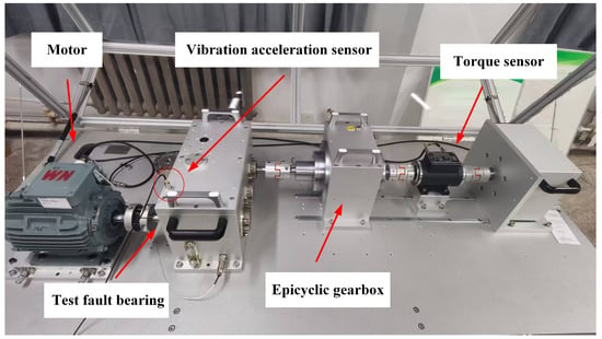
Figure 7. Gearbox bearing failure simulation test bench.

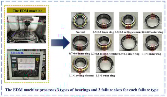
Figure 8. Bearing fault diagram.

Table 2. Test parameters for bearing operating conditions.

Operating Conditions	Rotational Speed (r/min)	Load (N·m)
Condition 1	1010	6
Condition 2	1511	11
Condition 3	1812	23
Condition 4	2115	33

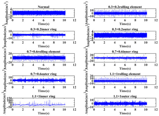
Figure 9. Time-domain diagrams of bearing vibration signals under different fault types.

The signals were preprocessed using an overlapping sampling [30,31] method for slicing, with a window length of 2048 and an overlap ratio of 50%, until the entire signal was traversed by sliding window segmentation. Ultimately, each type of fault was divided into 126 samples, which were then split into a training set and a test set in a 7:3 ratio [32]. The data classification categories and labels are shown in Table 3. Vibration signals from bearings with different fault severities were converted into two-dimensional feature images using GST and GADF, as shown in Figure 10 and Figure 11. Each bearing data sample corresponds to a GST time–frequency feature image and a GADF time-domain feature image, which are compressed into a three-channel image with a resolution of 64 × 64. Through two distinct transformation methods, the time-domain signals are decomposed into different feature components, thereby providing relatively rich time–frequency domain feature information for the proposed model.

Table 3. Samples of different fault types.

Label	State Type	Fault Degree	Sample
1	Normal	—	126
2	Inner ring	0.3 × 0.2	126
3	Inner ring	0.7 × 0.6	126
4	Inner ring	1.1 × 1	126
5	Outer ring	0.3 × 0.2	126
6	Outer ring	0.7 × 0.6	126
7	Outer ring	1.1 × 1	126
8	Rolling	0.3 × 0.2	126
9	Rolling	0.7 × 0.6	126
10	Rolling	1.1 × 1	126

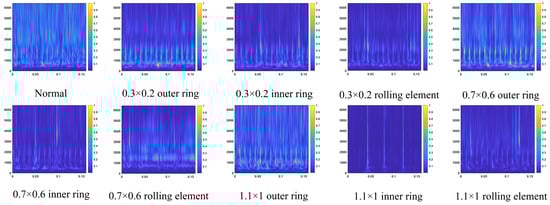
Figure 10. Feature map after GST processing of time-series signals.

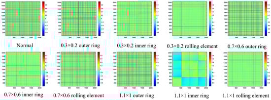
Figure 11. Feature map after GADF processing of time-series signals.

4.2. Model Performance Analysis

The performance of the proposed model was evaluated by comparing it with the WDCNN [33], dual-channel LeNet-5 [34], VMD-GRU-Transformer [35], Transformer [36], and LiConvFormer [37] models. Each model was trained and tested five times, and the macro-average performance metrics were calculated. The corresponding results are shown in Table 4. The proposed model achieved macro-average precision, recall, and F1-score all above 99%, demonstrating superior performance compared to other benchmark models with varying degrees of improvement in network performance. The network performance of the proposed model significantly outperformed the other three models. As shown in the confusion matrix in Figure 12, the proposed model exhibited only one misclassification between inner-circle 1 mm faults and normal samples, whereas the other three models misclassified multiple fault types. Both performance metrics and confusion matrix results demonstrate that the proposed method achieves high fault recognition performance.

Table 4. Performance metrics comparison of models.

Model	Precision	Recall	F1
The proposed model	99.57	99.53	99.52
WDCNN	95.27	95.11	95.12
Dual-channel LeNet-5	99.07	99	99.01
VMD-GRU-Transformer	96.75	96.68	96.66
Transformer	96.61	96.05	96.02
LiConvFormer	98.79	98.68	98.67

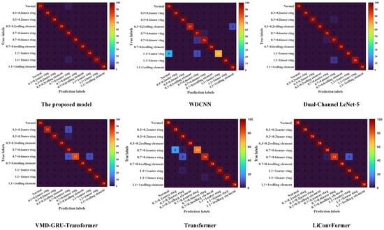
Figure 12. Comparison of the confusion matrix.

To further validate the effectiveness of the multi-feature, multi-channel network model, an ablation study was designed for comparative analysis. Using bearing fault signals under operating conditions of 1511 r/min rotational speed and 11 N·m torque as an example, we designed four models with two-dimensional feature map inputs and compared them with the model proposed in this paper, adhering to the principle of controlling variables. The four model schemes were as follows: ① a CNN-Transformer network model with single GADF time-domain feature input; ② a CNN-Transformer network model with single GST time–frequency feature input; ③ a dual-channel CNN-Transformer network model with the same GADF time-domain feature input; ④ a dual-channel CNN-Transformer network model with the same GST time–frequency feature input, and ⑤ a dual-channel CNN-Transformer network model with reversed attention mechanism, based on GST and GADF time–frequency feature inputs. The different model schemes are shown in Figure 13.

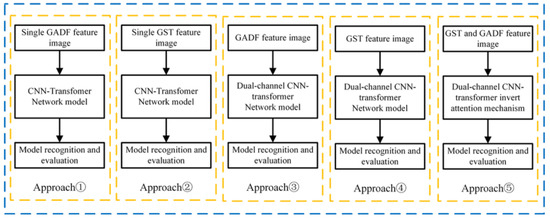
Figure 13. Scheme of different models.

Using signals with varying degrees of fault severity as inputs for the four models, five training and testing iterations were conducted. The model accuracy is shown in Figure 14 and Table 5. Schemes ① and ②, which used a single feature map as input, had average accuracy rates of 96.74 ± 0.61% and 97.00 ± 0.44%, respectively. Schemes ③ and ④, which used the same feature map with dual-channel input, had average accuracy rates of 98.16 ± 0.56% and 98.26 ± 0.55%, respectively. After reversing the attention mechanism in the original model, Model ⑤ achieved a mean accuracy of 98.34 ± 0.26%. The model that combines two different feature maps can obtain different time–frequency domain feature information. After adaptive fusion by the dual-channel CNN-Transfomer-CAM model, the average accuracy rate for identifying different fault levels was as high as 99.53 ± 0.22%. Compared with the other four network models, the average accuracy rates improved by 2.79%, 2.53%, 1.37%, 1.27% and 1.19%, respectively, further validating the effectiveness of the proposed multi-feature multi-channel network model.

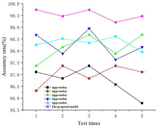
Figure 14. Test result of different models.

Table 5. Accuracy rates of different models.

Model	Average Accuracy	Standard Deviation	95% Confidence Interval
1	96.74	0.61	(95.98, 97.50)
2	97.00	0.44	(96.45, 97.55)
3	98.16	0.56	(97.47, 98.86)
4	98.26	0.55	(97.58, 98.94)
5	98.34	0.26	(98.02, 98.66)
6	99.53	0.22	(99.26, 99.80)

4.3. Robustness Verification Under Noise and Few Samples

This section analyzes the proposed model under two conditions: noise interference and few samples. First, Gaussian white noise with signal-to-noise ratios (SNR) of 0 dB, 2 dB, and 4 dB [38] was added to the measured signals to simulate industrial noise interference. The injection method for Gaussian white noise is based on the additive principle of signal-to-noise ratio. The average power of the original signal is calculated, and the required noise power is derived according to the target SNR. By scaling the amplitude of standard Gaussian noise, the noise power is adjusted to meet the design requirements. Finally, the noise is superimposed with the original signal in the time domain to generate the noisy signal. Five tests were conducted on signals with different SNRs, and the recognition accuracy is shown in Figure 15. As the signal-to-noise ratio decreased, the model’s recognition accuracy also showed a gradual decline. This is because noise disrupts the integrity and separability of fault features, making it difficult for the model to extract complete features. However, even under 0 dB noise interference, the average recognition accuracy of the proposed model remained above 97%. To visualize the classification performance of the model, t-SNE plots were generated for four signals with different signal-to-noise ratios. As shown in Figure 16, as the signal-to-noise ratio increased, labels of different fault severities exhibited distinct clustering distributions in the feature space, indicating that the model can effectively distinguish between different types of fault states. When the signal-to-noise ratio was 0 dB, a small degree of overlap in the feature space was observed between labels of the rolling element fault with a severity of 0.7 mm and those of the inner race fault with a severity of 0.3 mm, while labels of the remaining fault types maintained high compactness without significant distribution confusion. This result indicates that although the discriminability of some fault types decreases under noise interference, the proposed model can still mitigate the impact of noise to a certain extent.

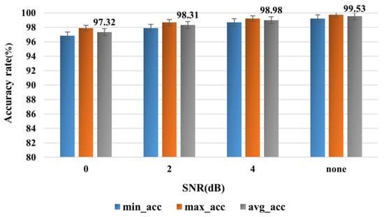
Figure 15. Test set accuracy after adding different SNR noises.

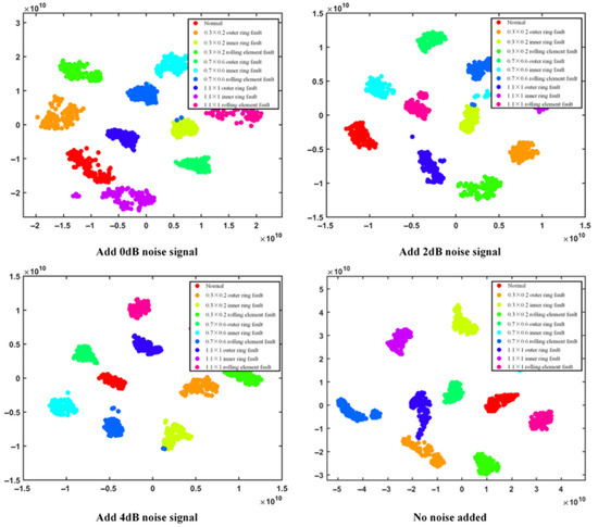
Figure 16. T-SNE plots of model classification results at different signal-to-noise ratios.

For neural network models, the input of different training samples also influences the diagnostic outcomes. When training samples are limited, models often tend to become more complex in an attempt to improve performance, which can easily lead to overfitting. This model uses multi-feature two-dimensional images as input and integrates a CNN-Transformer-CAM network model, which has certain advantages in handling a small number of training samples. To verify the superiority of the proposed model in analyzing small sample data, the training set was set to 20%, 30%, and 50% of the total samples, and the model was trained and tested five times. The model’s recognition accuracy is shown in Figure 17. Even with reduced training samples, the proposed model maintained a high accuracy rate. When the training samples accounted for only 20% of the total, the average accuracy rate remained above 94%. The experimental results indicate that the proposed model demonstrates excellent robustness and noise resistance under noisy and small-sample conditions.

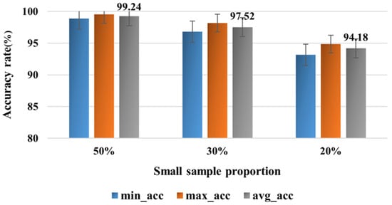
Figure 17. Recognition accuracy under different small samples.

4.4. Generalizability Verification Under Different Operating Conditions

This section uses the bearing failure dataset collected by the aforementioned laboratory and the CWRU bearing failure dataset to verify and analyze the generalization ability of the proposed model.

First, four different fault signals collected in the laboratory under different operating conditions were used for verification. The operating conditions simulated in this section included three constant conditions: ① speed of 1010 r/min, ② speed of 1812 r/min, and ③ speed of 2115 r/min. In addition, there were three variable conditions: condition ④ with a speed of 1511 r/min was used as the training set, and the signals contained in conditions ①, ②, and ③ were used as the corresponding test set. The proposed network model was tested five times under different operating conditions, and the corresponding recognition accuracy rates are shown in Figure 18. The average accuracy rates under the three constant operating conditions were all above 99%, respectively. For the three variable operating conditions, as the speed increased and the torque increased, the operating conditions became more severe, and the differences between the source domain and the target domain increased, making it more difficult for the proposed model to identify, resulting in a decreasing trend in recognition accuracy. Due to the adaptive fusion of local and global information of different time–frequency features by the proposed dual-channel model, the average accuracy rate could still be maintained above 97%. This indicates that the proposed model can maintain a high recognition accuracy under different constant and variable operating conditions, demonstrating strong generalization capabilities.

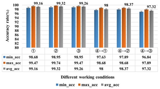
Figure 18. Recognition accuracy in other working conditions.

Validation and analysis were conducted using the CWRU bearing fault dataset. The experimental conditions consisted of four operating speeds: ① 1797 r/min, ② 1772 r/min, ③ 1750 r/min, and ④ 1730 r/min [39]. Vibration signals from the drive end corresponding to different fault types were collected using sensors, with bearing fault diameters of 0.1778 mm, 0.3556 mm, and 0.5334 mm [40]. The four operating condition samples were processed using the data preprocessing methods described earlier, and five tests were conducted for each. The recognition accuracy of the proposed model is shown in Figure 19. For the four different operating conditions, the average recognition accuracy rates of the proposed model were 99.74%, 99.53%, 99.4%, and 99.27%, respectively, all exceeding 99%. We analyzed the results corresponding to the lowest accuracy rate of the model under different operating conditions, as shown in Figure 20: Under operating condition ①, the proposed model exhibited the fewest prediction errors for samples with different fault severities, with only one error occurring in the rolling element fault sample of 0.1778 mm. Under operating condition ④, the number of prediction errors was the highest, reaching four; while operating conditions ② and ③ had 2 and 3 errors, respectively. However, for all four operating conditions, the proposed model still achieved a minimum identification evaluation accuracy of over 98.5%, indicating that the proposed model maintains excellent generalization performance under different operating conditions at CWRU.

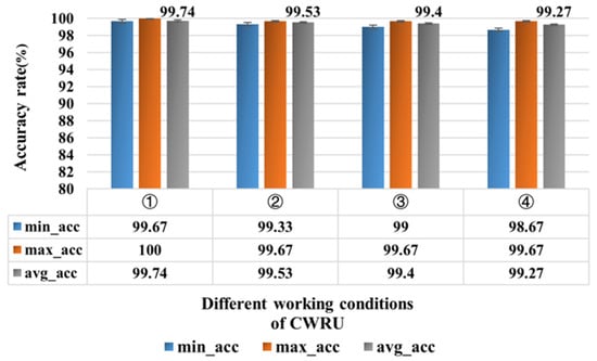
Figure 19. Accuracy under different working conditions of CWRU.

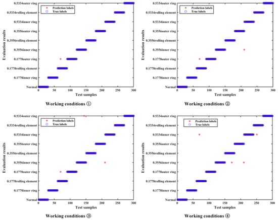
Figure 20. Evaluation results under different working conditions of CWRU.

5. Conclusions

Aiming at the limitations of existing bearing fault diagnosis methods in handling non-stationary signals, extracting complex features, and resisting interference, this paper proposed a dual-channel CNN-Transformer-CAM fault diagnosis model based on deep multi-feature fusion. The model constructs a two-dimensional input that combines informational completeness and discriminative power by fusing the time-domain features from the Gramian Angular Difference Field (GADF) and the time–frequency features from the generalized S-transform (GST). The model employs a dual-channel parallel convolutional architecture to extract local multi-scale features, integrates a Transformer encoder to capture global long-range dependencies, and finally utilizes a cross-attention mechanism to achieve adaptive weighted feature fusion, significantly enhancing its capability to represent and classify complex fault patterns. Based on the analysis and validation across multiple datasets, the following conclusions can be drawn:

• Compared with models such as WDCNN, dual-channel LeNet-5, and VMD-GRU-Transformer, the proposed model demonstrates superior performance, with the macro-average precision, recall, and F1 score all exceeding 99%. When compared with single-channel and other dual-channel network models, the proposed model achieved an accuracy rate of 99.53% for identifying different fault severities, significantly outperforming the other four network models, thereby fully validating the effectiveness of the multi-feature multi-channel network model.
• The model maintains excellent robustness under noise interference and few samples. Even under 0 dB noise interference, the average identification accuracy of the model remained above 97%. When the training samples accounted for only 20%, the average identification accuracy was still above 94%, demonstrating good stability under few sample conditions.
• The model exhibits outstanding generalization performance under different test conditions. For both constant and variable conditions, the model achieved an average recognition accuracy rate of 98.57%. In the CWRU bearing dataset, the model achieved an average recognition accuracy rate exceeding 99% under different conditions, further validating its adaptability across diverse operational environments.

Although the proposed model demonstrates superior performance in bearing fault diagnosis, the following directions warrant further exploration. The current work primarily addresses steady-state and limited variable operating conditions, as well as single-type noise interference. However, real industrial environments often involve compound, non-Gaussian, and time-varying strong noise interference. We acknowledge the limitations of the current study. Future work will focus on the complex and diverse noise interference and operating scenarios in real industrial settings, conducting more challenging model validation and adaptation efforts.

References

- Wan, S.; Zhao, X.; Wang, Y.; Zhang, B.; Zhang, X.; Gu, X. A Fault Diagnosis Method for Variable Speed Gearbox Bearing Based on SET Improved Multi-Source Ridge Line. Measurement 2023, 214, 112758. [Google Scholar] [CrossRef]
- Wang, B.; Ding, C. Transient Feature Identification from Internal Encoder Signal for Fault Detection of Planetary Gearboxes under Variable Speed Conditions. Measurement 2021, 171, 108761. [Google Scholar] [CrossRef]
- Cui, L.; Liu, Y.; Zhao, D. Adaptive Singular Value Decomposition for Bearing Fault Diagnosis under Strong Noise Interference. Meas. Sci. Technol. 2022, 33, 095002. [Google Scholar] [CrossRef]
- Hu, A.-J.; Zhu, Y. Instantaneous Frequency Estimation of a Rotating Machinery Based on an Improved Peak Search Method. Zhendong Yu Chongji J. Vib. Shock 2013, 32, 113–117. [Google Scholar]
- Guo, Z.; Du, W.; Li, C.; Guo, X.; Liu, Z. Fault Diagnosis of Rotating Machinery with High-Dimensional Imbalance Samples Based on Wavelet Random Forest. Measurement 2025, 248, 116936. [Google Scholar] [CrossRef]
- Bie, F.; Du, T.; Lyu, F.; Pang, M.; Guo, Y. An Integrated Approach Based on Improved CEEMDAN and LSTM Deep Learning Neural Network for Fault Diagnosis of Reciprocating Pump. IEEE Access 2021, 9, 23301–23310. [Google Scholar] [CrossRef]
- He, S.; Xiao, L.; Wang, Y.; Liu, X.; Yang, C.; Lu, J.; Gui, W.; Sun, Y. A Novel Fault Diagnosis Method Based on Optimal Relevance Vector Machine. Neurocomputing 2017, 267, 651–663. [Google Scholar] [CrossRef]
- Zheng, J.; Pan, H.; Cheng, J. Rolling Bearing Fault Detection and Diagnosis Based on Composite Multiscale Fuzzy Entropy and Ensemble Support Vector Machines. Mech. Syst. Signal Process. 2017, 85, 746–759. [Google Scholar] [CrossRef]
- Li, H.; Wu, X.; Liu, T.; Li, S.; Zhang, B.; Zhou, G.; Huang, T. Composite Fault Diagnosis for Rolling Bearing Based on Parameter-Optimized VMD. Measurement 2022, 201, 111637. [Google Scholar] [CrossRef]
- Yang, J.; Li, X. An Integrated Mechanical Fault Diagnosis Framework Using Improved GOOSE-VMD, RobustICA, and CYCBD. Machines 2025, 13, 631. [Google Scholar] [CrossRef]
- Yuan, B.; Lei, L.; Chen, S. Optimized Variational Mode Decomposition and Convolutional Block Attention Module-Enhanced Hybrid Network for Bearing Fault Diagnosis. Machines 2025, 13, 320. [Google Scholar] [CrossRef]
- Ye, M.; Yan, X.; Hua, X.; Jiang, D.; Xiang, L.; Chen, N. MRCFN: A Multi-Sensor Residual Convolutional Fusion Network for Intelligent Fault Diagnosis of Bearings in Noisy and Small Sample Scenarios. Expert Syst. Appl. 2025, 259, 125214. [Google Scholar] [CrossRef]
- Zhang, W.; Peng, G.; Li, C.; Chen, Y.; Zhang, Z. A New Deep Learning Model for Fault Diagnosis with Good Anti-Noise and Domain Adaptation Ability on Raw Vibration Signals. Sensors 2017, 17, 425. [Google Scholar] [CrossRef]
- Zhang, Z.; Jiao, Z.; Li, Y.; Shao, M.; Dai, X. Intelligent Fault Diagnosis of Bearings Driven by Double-Level Data Fusion Based on Multichannel Sample Fusion and Feature Fusion under Time-Varying Speed Conditions. Reliab. Eng. Syst. Saf. 2024, 251, 110362. [Google Scholar] [CrossRef]
- Zhang, S.; Liu, Z.; Chen, Y.; Jin, Y.; Bai, G. Selective Kernel Convolution Deep Residual Network Based on Channel-Spatial Attention Mechanism and Feature Fusion for Mechanical Fault Diagnosis. ISA Trans. 2023, 133, 369–383. [Google Scholar] [CrossRef]
- Yao, Q.; Qin, Y.; Wang, X.; Qian, Q. Multiscale Domain Adaption Models and Their Application in Fault Transfer Diagnosis of Planetary Gearboxes. Eng. Appl. Artif. Intell. 2021, 104, 104383. [Google Scholar] [CrossRef]
- Spirto, M.; Melluso, F.; Nicolella, A.; Malfi, P.; Cosenza, C.; Savino, S.; Niola, V. A Comparative Study between SDP-CNN and Time–Frequency-CNN Based Approaches for Fault Detection. J. Dyn. Monit. Diagn. 2025. [Google Scholar] [CrossRef]
- Wang, S.; Zhang, J. An Intelligent Process Fault Diagnosis System Based on Andrews Plot and Convolutional Neural Network. J. Dyn. Monit. Diagn. 2022, 1, 127–138. [Google Scholar] [CrossRef]
- Zhang, Q.; Deng, L. An Intelligent Fault Diagnosis Method of Rolling Bearings Based on Short-Time Fourier Transform and Convolutional Neural Network. J. Fail. Anal. Prev. 2023, 23, 795–811. [Google Scholar] [CrossRef]
- Peng, C.; Peng, J.; Wang, Z.; Wang, Z.; Chen, J.; Xuan, J.; Shi, T. Adaptive Fault Diagnosis of Railway Vehicle On-Board Controller with Large Language Models. Appl. Soft Comput. 2025, 185, 113919. [Google Scholar] [CrossRef]
- Wang, Z.; Chen, J.; Wang, C.; Peng, C.; Xuan, J.; Shi, T.; Zuo, M. CNC-VLM: An RLHF-Optimized Industrial Large Vision-Language Model with Multimodal Learning for Imbalanced CNC Fault Detection. Mech. Syst. Signal Process. 2026, 245, 113838. [Google Scholar] [CrossRef]
- Chen, L.; Xu, D.; Yang, L.; Ng, C.-T.; Fu, J.; He, Y.; He, Y. Classification and Identification of Extreme Wind Events by CNNs Based on Shapelets and Improved GASF-GADF. J. Wind Eng. Ind. Aerodyn. 2024, 253, 105852. [Google Scholar] [CrossRef]
- Xiong, L.; He, M.; Hu, C.; Hou, Y.; Han, S.; Tang, X. Image Presentation and Effective Classification of Odor Intensity Levels Using Multi-Channel Electronic Nose Technology Combined with GASF and CNN. Sens. Actuators B Chem. 2023, 395, 134492. [Google Scholar] [CrossRef]
- Chen, Y.; Zhang, D.; Deng, C.; Song, Y. Integrated Learning Method of Gramian Angular Field and Optimal Feature Channel Adaptive Selection for Bearing Fault Diagnosis. In Proceedings of the 2022 8th International Conference on Control, Automation and Robotics (ICCAR), Xiamen, China, 8–10 April 2022; IEEE: Piscataway, NJ, USA, 2022; pp. 209–217. [Google Scholar]
- Stockwell, R.G.; Mansinha, L.; Lowe, R.P. Localization of the Complex Spectrum: The S Transform. IEEE Trans. Signal Process. 2002, 44, 998–1001. [Google Scholar] [CrossRef]
- Liu, W.; Han, M.; Chen, L. Bearing Fault Diagnosis Based on Generalized S Transform Denoising and Convolutional Neural Network. In Proceedings of the 2018 Chinese Intelligent Systems Conference, Wenzhou, China, 13–14 October 2018; Springer: Singapore, 2018; pp. 425–432. [Google Scholar]
- Wang, X.; Mao, D.; Li, X. Bearing Fault Diagnosis Based on Vibro-Acoustic Data Fusion and 1D-CNN Network. Measurement 2021, 173, 108518. [Google Scholar] [CrossRef]
- Vaswani, A.; Shazeer, N.; Parmar, N.; Uszkoreit, J.; Jones, L.; Gomez, A.N.; Kaiser, Ł.; Polosukhin, I. Attention Is All You Need. Adv. Neural Inf. Process. Syst. 2017, 30, 1–11. [Google Scholar]
- Zhang, Y.; Lv, C. TinySegformer: A Lightweight Visual Segmentation Model for Real-Time Agricultural Pest Detection. Comput. Electron. Agric. 2024, 218, 108740. [Google Scholar] [CrossRef]
- Kumar, R.; Anand, R.S. A Multi-Scale Deep Neural Networks for Early Fault Diagnosis in Rolling Ball Bearings. Soft Comput. 2025, 29, 3603–3615. [Google Scholar] [CrossRef]
- Zhang, X.; Liu, G.; Zhou, Y.; Jia, L. An Adaptive Fully Convolutional Network for Bearing Fault Diagnosis under Noisy Environments. Rev. Sci. Instrum. 2024, 95, 045104. [Google Scholar] [CrossRef]
- Yang, Z.; Yang, R.; Huang, M. Rolling Bearing Incipient Fault Diagnosis Method Based on Improved Transfer Learning with Hybrid Feature Extraction. Sensors 2021, 21, 7894. [Google Scholar] [CrossRef] [PubMed]
- Song, X.; Cong, Y.; Song, Y.; Chen, Y.; Liang, P. A Bearing Fault Diagnosis Model Based on CNN with Wide Convolution Kernels. J. Ambient Intell. Humaniz. Comput. 2022, 13, 4041–4056. [Google Scholar] [CrossRef]
- Wan, L.; Chen, Y.; Li, H.; Li, C. Rolling-Element Bearing Fault Diagnosis Using Improved LeNet-5 Network. Sensors 2020, 20, 1693. [Google Scholar] [CrossRef]
- Lei, W.; Dong, X.; Cui, F.; Huang, G. A Remaining Useful Life Prediction Method for Rolling Bearings Based on Hierarchical Clustering and Transformer–GRU. Appl. Sci. 2025, 15, 5369. [Google Scholar] [CrossRef]
- Yang, Z.; Cen, J.; Liu, X.; Xiong, J.; Chen, H. Research on Bearing Fault Diagnosis Method Based on Transformer Neural Network. Meas. Sci. Technol. 2022, 33, 085111. [Google Scholar] [CrossRef]
- Yan, S.; Shao, H.; Wang, J.; Zheng, X.; Liu, B. LiConvFormer: A Lightweight Fault Diagnosis Framework Using Separable Multiscale Convolution and Broadcast Self-Attention. Expert Syst. Appl. 2024, 237, 121338. [Google Scholar] [CrossRef]
- Xu, M.; Yu, Q.; Chen, S.; Lin, J. Rolling Bearing Fault Diagnosis Based on CNN-LSTM with FFT and SVD. Information 2024, 15, 399. [Google Scholar] [CrossRef]
- Wang, F.; Song, G. Monitoring of Multi-Bolt Connection Looseness Using a Novel Vibro-Acoustic Method. Nonlinear Dyn. 2020, 100, 345–360. [Google Scholar] [CrossRef]
- Zheng, J.; Yuan, Y.; Zou, L.; Deng, W.; Guo, C.; Zhao, H. Study on a Novel Fault Diagnosis Method Based on VMD and BLM. Symmetry 2019, 11, 747. [Google Scholar] [CrossRef]
Disclaimer/Publisher’s Note: The statements, opinions and data contained in all publications are solely those of the individual author(s) and contributor(s) and not of MDPI and/or the editor(s). MDPI and/or the editor(s) disclaim responsibility for any injury to people or property resulting from any ideas, methods, instructions or products referred to in the content. |
© 2026 by the authors. Licensee MDPI, Basel, Switzerland. This article is an open access article distributed under the terms and conditions of the Creative Commons Attribution (CC BY) license.