Abstract
The integration of axial flux motors into canned motor pumps offers a promising approach to overcome the efficiency and size limitations of traditional designs, particularly in critical sectors like aerospace. However, the hydrodynamics in magnetic gap between the stator and rotor are poorly understood. This study investigates the effect of magnetic gap on performance and internal flow. Six magnetic gap schemes are developed, ranging from 0.2 to 1.2 mm. Numerical simulations are conducted, and simulation results showed good agreement with experimental data. The magnetic gap exhibits a non-linear effect on performance. The peak head coefficient occurs at a 0.4 mm gap and maximum efficiency at 1.0 mm. At a 0.2 mm gap, strong viscous shear forces increase disk friction loss and create high-vorticity flow. As the gap widens, flow transitions from viscosity-dominated to inertia-dominated, leading to a more ordered flow structure. The blade passing frequency is the dominant frequency. For a gap of 0.8 mm, the pressure fluctuation intensity is lowest. By analyzing performance, head coefficient, velocity, vorticity, entropy production, and pressure fluctuations, a gap of 0.8 mm is identified as the optimal design. This study provides critical guidance for optimizing the design of axial flux canned motor pumps.
1. Introduction
Exceptional safety and reliability in fluid conveyance are paramount for demanding applications in the petrochemical, nuclear, aerospace, and biopharmaceutical sectors [1,2]. Owing to its inherent sealed design, the canned motor pump has emerged as a core technological apparatus for guaranteeing the secure conveyance of hazardous media. Nevertheless, this inherent advantage of its canned motor architecture concurrently presents a persistent technical challenge: low hydraulic efficiency and large size. This severely constrains its application and advancement in high-efficiency and compact systems. To address this challenge, a high-power-density axial flux motor replaces conventional radial flux motors, and an integrated design unifying the permanent magnet rotor and the impeller is adopted [3]. This design optimizes structural compactness and creates a submerged passage within the magnetic gap between the stator and rotor, as illustrated in Figure 1. In the magnetic gap, the fluid is subjected not only to high-speed rotational shear and complex geometric constraints but also to direct modulation by the electromagnetic field. However, a comprehensive understanding of the flow dynamics and energy dissipation mechanisms in this multiphysics region is still lacking. Therefore, this study aims to address the knowledge gap by conducting a systematic investigation of the flow field in the magnetic gap of submerged axial flux motors in centrifugal pumps. The primary objectives are to elucidate the governing flow dynamics and their impact on performance. This study provides a scientific basis and design criteria for developing novel axial flux canned motor pumps that combine high safety with significantly enhanced hydraulic efficiency and compactness.
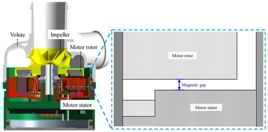
Figure 1.
Magnetic gap in submerged axial flux motors.
Research on canned motor pumps has long garnered significant attention. Numerical simulation has emerged as a primary investigative tool, effectively revealing the characteristics of confined internal flow fields. Most existing research has focused on conventional radial flux canned motor pumps, with extensive investigations spanning various aspects. Regarding hydraulic characteristics, Zhu et al. [4] investigated the strong rotor–stator interaction in a canned motor pump operating under part-load conditions. In multiphysics coupling, Tinni et al. [5] combined electromagnetic and thermal analytical models to investigate the electrical performance and stator life of shielded motors by predicting peak winding temperatures under various operating conditions. Huang et al. [6] analyzed the performance of permanent magnet shielded motors in circulation pumps under different control strategies. Zhou et al. [7] addressed the vibration and noise issues of shielded pump motors using numerical simulation methods that involve electromagnetic–fluid–mechanical multiphysics coupling. For operating characteristics, Kanyolo et al. [8] analyzed the torque characteristics and motor behavior during the start-up process of reactor coolant pumps. In recent years, axial flux motors have gained significant attention, as their potential for higher performance could overcome the efficiency and power density bottlenecks of traditional radial flux designs. This inherent compactness, characterized by a significantly shorter axial length, often reduces the overall motor length by approximately half compared to radial flux designs of comparable power. This size advantage is crucial for integrated pump designs, as it effectively addresses the size limitations of traditional configurations and offers significant value in space-constrained applications. However, relevant research has primarily focused on the electromagnetic and mechanical performance analysis of these motors. Pang et al. [9] proposed a wirelessly controlled axial flux motor for micropumps. They found that this design offered improved output torque and efficiency compared to similar radial flux motors. Eker et al. [10] conducted comparative experiments on axial flux and radial flux motors. Their research analyzed steady-state and transient performance, efficiency, and power factor under various load conditions. Ai et al. [11,12,13] introduced an axial flux motor structure for cryogenic liquid immersion pumps. They compared the rotor suspension force changes with radial flux motors and analyzed the internal electromagnetic force characteristics of this specific structure. Gadiyar et al. [14] explored the integrated design of hydraulic pumps with axial flux motors. Zhang et al. [15] investigated the impact of geometric parameters on friction and viscous losses in axial flux permanent magnet motors used in electronic coolant pumps. They concluded that axial flux motors exhibit superior torque performance compared to radial flux motors. Despite the existing literature comprehensively validating the performance advantages of axial flux motors from an electromagnetic perspective, there has been scant discussion regarding the hydraulic issues arising from their integration. This is particularly true for submerged axial motors, where the influence of the magnetic gap on hydraulic performance and the internal flow field has rarely been explored. This research gap represents a significant theoretical shortcoming, hindering the development of a new generation of high-efficiency axial flux canned pumps.
Gap flow is a fundamental physical factor affecting the energy performance and operational stability of various pumping equipment. Existing research widely confirms that the complex vortex evolution and energy dissipation resulting from the mixing of leakage flow with the main flow fundamentally limit hydraulic performance and structural reliability. Regarding energy performance, Fan et al. [16] and Gu et al. [17] systematically investigated the impact of increased gaps, caused by seal ring wear, on energy loss in multi-stage centrifugal pumps. Zhan et al. [18] analyzed the influence of radial clearance on leakage and viscous friction losses in gear pumps. Concerning dynamic characteristics, fluid–structure interaction between the gap flow and main flow is crucial in inducing pressure fluctuations, unsteady hydraulic loads, and vibrations. Hou et al. [19] analyzed the dynamic hydraulic loads within the gap flow channels during the runaway oscillation of pump turbines. Zheng et al. [20] and Guang et al. [21] analyzed the spectral characteristics of pressure fluctuations induced by gap flow in centrifugal pumps. Li et al. [22] reduced the amplitude of pressure fluctuations at blade passing frequency and its harmonics in centrifugal pumps through optimized gap design, thereby suppressing vibration and noise. Liang et al. [23] found that the fluid–structure interaction effect caused by the rotor meshing gap and radial gap in the hydrogen circulation pump cavity resulted in a dominant pressure fluctuation frequency of twice the rotational frequency. Regarding geometric parameters, pump performance and stability are highly sensitive to the specific geometry of the gaps. Several researchers have focused on clarifying how these geometric parameters influence performance. Li et al. [24] investigated the effect of gap thickness on the axial force and flow field in pump turbines. To explore the impact of blade root leading and trailing edge gaps on the hydraulic performance of axial flow pumps, Li et al. [25] analyzed the energy characteristics and internal flow field structures under four different blade root gaps and two hub geometries. Zhou et al. [26] analyzed how the axial gap in vortex pumps affects the internal flow field and external characteristics. Jia et al. [27] analyzed the influence of the incidence angle on the pump’s external characteristics and internal flow features. Oro et al. [28] studied the effect of radial gap size on unsteady velocity field fluctuations within the pump. Liu et al. [29] investigated the influence of gap flow on the head coefficient, efficiency, average radial offset of vortices, and axial velocity uniformity. However, the extensive research discussed above primarily focuses on conventional gaps arising from mechanical fits or sealing requirements, such as those found in seal rings or between impellers and pump casings. The core magnetic gap in the axial flux canned pump, which is the subject of this paper, is fundamentally different. It is not a product of mechanical fitting but rather constitutes a unique flow passage formed by the integrated design of the permanent magnet rotor and impeller. Therefore, existing gap flow theories are not directly applicable. Addressing this critical theoretical shortcoming, this study pioneers a systematic investigation into the unique unsteady flow patterns, energy dissipation distribution in this magnetic gap, and their coupled influence on hydraulic performance and pressure fluctuations. This research fills a significant gap in current knowledge, providing foundational insights and design criteria essential for developing a new generation of high-efficiency axial flux canned pumps.
This study focuses on submerged axial flux motor centrifugal pumps, specifically examining the magnetic gap. Six distinct magnetic gap configurations are designed. Utilizing a combined approach of numerical simulation and experimental methods, we comprehensively investigated the influence of the magnetic gap on hydraulic performance and internal flow characteristics.
2. Numerical Simulation
2.1. Pump Parameters
This study focuses on a submerged axial-flux centrifugal pump, characterized by the integrated design of its impeller and permanent magnet rotor, as shown in Figure 2. The design flow rate (Qd) is 9 m3/h and the rotational speed (n) is 5200 rpm. In this innovative structure, the motor stator and rotor are axially arranged in parallel, forming a unique magnetic gap. This magnetic gap is not only a critical region for transmitting electromagnetic energy but its complex fluid dynamics also influence hydraulic performance, mechanical efficiency, and operational reliability.
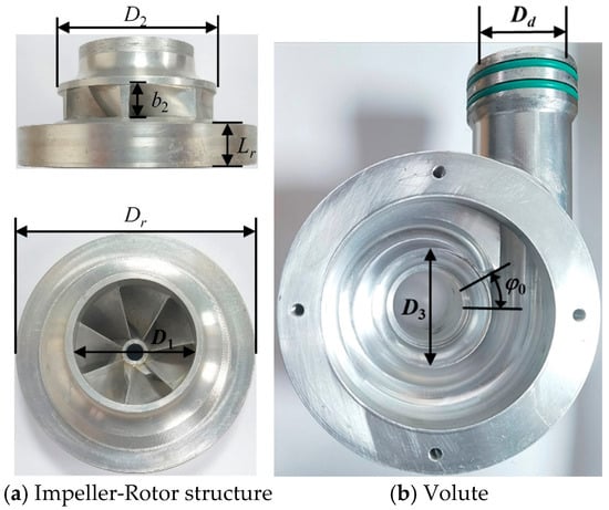
Figure 2.
Pump model.
Traditionally, magnetic gap design has primarily focused on electromagnetic performance, often simplifying or neglecting its critical hydraulic effects, such as leakage, shear dissipation, and pressure fluctuation. To accurately isolate and focus on investigating the influence of the magnetic gap on hydraulic performance, this study constructed an equivalent physical model for testing and analysis. This model replicates the integrated impeller–rotor assembly and other core hydraulic components, such as the volute, exactly as found in the actual pump. The magnetic gap in the original design is represented by the axial clearance between the rear shroud and the stationary casing wall. An external motor drives the impeller–rotor assembly, enabling a pure and controllable investigation of the fluid dynamics in this axial clearance and their impact on performance, free from direct electromagnetic field interference. This paper primarily focuses on the hydraulic design aspect, while electromagnetic design details and their coupling with the fluid field fall within the scope of motor design, typically addressed in a more comprehensive multiphysics optimization. We plan to address the coupled electromagnetic–hydraulic performance in our future research, building upon the hydrodynamic insights gained from this current work, at which point the motor’s specific parameters and topology will be detailed.
Based on this simplified model and to systematically investigate the influence of the magnetic gap, six distinct magnetic gap configurations are established, maintaining all other geometric parameters of the impeller and volute constant. The investigated gap values ranged from 0.2 mm to 1.2 mm, specifically including 0.2, 0.4, 0.6, 0.8, 1.0, and 1.2 mm. The geometric parameters of the pump are presented in Table 1. This research aims to elucidate the intrinsic influence of the magnetic gap, as a critical geometric parameter, on hydraulic characteristics, thereby offering theoretical insights and data support for the fluid–magnetic coupled optimal design of next-generation axial-flux shielded pumps.

Table 1.
Main geometrical parameters.
2.2. Control Equations
Based on the Reynolds-Averaged Navier–Stokes equations, the centrifugal pump is numerically simulated using the commercial software ANSYS CFX 2020. The continuity and momentum equations are shown in Equations (1) and (2).
where ρ is the density, t is the time, is the Reynolds-averaged velocity component, x is the coordinate, p is the Reynolds-averaged pressure, μ is the dynamic viscosity, is the Reynolds stress tensor, and fi is the external force.
The SST k-ω model is selected as the turbulence model for this study, as it combines the strengths of the k-ω and k-ε models while mitigating their respective drawbacks [30]. The working fluid is water at 25 °C, with a dynamic viscosity (μ) of 0.0008899 kg/m·s and a density of 997 kg/m3.
2.3. Boundary Conditions
A total pressure inlet boundary condition is applied, with the absolute pressure set at 1 atmospheric pressure and a turbulence intensity of 5%. The outlet is defined as a mass flow rate boundary condition. The internal flow is modeled using a Multiple Reference Frame approach, in which the impeller domain is assigned a rotating reference frame, while the volute and other domains are assigned a stationary reference frame. The steady-state results are used as the initial values for the unsteady calculations [31,32]. The convergence criterion for the numerical simulations is set to a residual target of 1 × 10⁻⁵ [33]. The impeller shrouds and blade surfaces are defined as rotating walls, subject to impermeable and no-slip boundary conditions.
2.4. Computational Grids
Figure 3 illustrates the mesh configuration of the fluid domain, which is partitioned into the front and rear chambers, the impeller, the volute, and the inlet and outlet extensions. Among these, the extension sections, chambers, and impeller are meshed with hexahedral grids using ANSYS ICEM CFD 2020. O-grid, C-grid, and Y-grid techniques are employed to topologically divide the flow passages to achieve high mesh quality. For the tongue area, its complex three-dimensional features make it difficult for a fully hexahedral mesh to meet the requirements of numerical computation. A hybrid tetrahedral–hexahedral mesh is generated using ANSYS Meshing 2020 with local refinement applied. The orthogonal quality of the hybrid mesh is greater than 0.7.
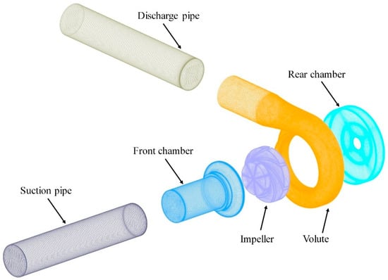
Figure 3.
Mesh of computational domains.
Notably, the mesh of the rear chamber, the primary focus of this study, primarily comprises two key regions: the rotor–stator axial gap and the rotor–casing radial gap. The Jacobian determinant and angles of all hexahedral meshes are greater than 0.5 and 18°, respectively, satisfying the requirements for high-precision resolution of the flow field. Boundary layers are added throughout the entire domain mesh to satisfy the requirements of the SST k-ω turbulence model for resolving low-Reynolds-number effects in the near-wall region.
2.5. Mesh Sensitivity
Figure 4 shows the relationship between mesh count and energy performance for the centrifugal pump. The data are derived from numerical simulations performed using ANSYS CFX 2020. To mitigate the impact of mesh density on numerical results, the energy performance of this pump is tested with six different mesh counts. When the mesh count reaches approximately 5.67 million, the calculated efficiency and head remain essentially unchanged.
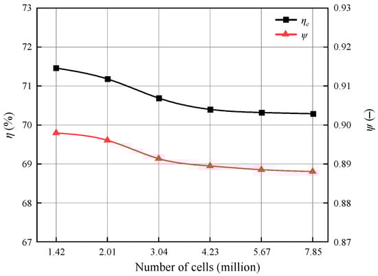
Figure 4.
Mesh independence.
To further evaluate the impact of mesh count on the calculation results, this research employs the Grid Convergence Index (GCI), as recommended by the American Society of Mechanical Engineers, to estimate mesh discretization errors. The GCI values for head and efficiency are 1.11% and 1.10%, respectively, confirming that the mesh meets convergence standards and supports the validity of the numerical simulations. Considering calculation accuracy and speed, the simulation used a mesh count of 5.67 million.
3. Experimental Setup and Validation
3.1. Experimental Setup
Figure 5 illustrates the experimental system for the high-speed pump in this study. It primarily consists of a test pump, a servo motor, pressure transmitters, a dynamic torque sensor, an electromagnetic flowmeter, valves, a tank, and a data acquisition system. During operation, the inlet valve is kept fully open to minimize inlet pipe resistance, and the flow rate is controlled by adjusting the opening of the outlet valve. The test apparatus is instrumented with a variety of sensors to acquire critical pump operating parameters in real time. A high-precision, multi-channel National Instruments data acquisition card is employed to facilitate the synchronous acquisition of measurement data from the various sensors.
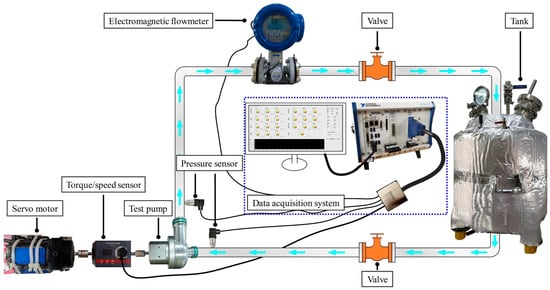
Figure 5.
Test setup for high-speed pumps.
Since the inlet and outlet pipe diameters are the same and the flow rate is identical, the flow velocities are also equal. Therefore, the dynamic pressure terms (kinetic energy terms) in the energy equation at both the inlet and outlet cancel each other out. As a result, the pump head (H) is determined through the application of Equation (3):
The calculation involves the pressures at the inlet (pin) and outlet (pout) of the test pump, denoted as ρ for density, g for gravitational acceleration, and ΔZ for the vertical distance between the inlet and outlet pressure sensors.
The shaft power (P) of the pump is computed using Equation (4):
Here, n represents the rotational speed, T denotes the shaft torque, and T0 is the unloaded shaft torque.
The efficiency (η) of the pump is derived using Equation (5):
The head coefficient is computed using Equation (6):
Here, u2 denotes the circumferential velocity at the blade outlet.
In the test setup, the systematic errors for the pressure sensors, electromagnetic flow meter, and speed/torque sensor are 0.1%, 0.5%, and 0.2%, respectively. To reduce experimental error and ensure accuracy, the experiment is repeated three times. The systematic uncertainties for the head and efficiency are 0.14% and 0.59%, respectively. In summary, the test setup meets the measurement requirements of the ISO 9906 international standard, ensuring the accuracy of the experiment.
3.2. Comparisons of Experimental and Numerical Energy Performances
Figure 6 displays the head coefficient and efficiency characteristic curves of the test pump, comparing the numerical simulation results with experimental data. The head coefficient (ψ) is a dimensionless parameter representing the ability to generate head, and efficiency (η) is a dimensionless measure of the energy conversion effectiveness. The horizontal axis represents the dimensionless flow rate, Q* = Q/Qd, where Q is the actual flow rate and Qd is the design flow rate. Overall, across the flow rate range of 0.3 Qd to 1.3 Qd, the simulated results demonstrate a strong agreement with the experimental data.
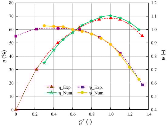
Figure 6.
Comparison of experimental and simulation results.
To quantify these differences, a detailed error analysis is performed. At 1.0 Qd, the simulated head coefficient is 0.889, which is 0.004 higher than the experimental value, corresponding to a relative error of 0.40%. The simulated efficiency is 70.32%, exceeding the experimental value by 1.76%. For other flow conditions, the average relative error in the head coefficient is 0.99%, with a maximum deviation of 2.32% occurring at 1.2 Qd. The mean absolute error for efficiency is 1.59%, with the largest negative deviation of −3.7% observed at 0.3 Qd. These results indicate that the numerical simulation deviations for both head coefficient and efficiency fall within acceptable engineering tolerances. The maximum overall error is consistent with the level of deviation typically found between simulations and experiments for similar turbomachinery [34]. This further validates that the current model and numerical methodology satisfy the accuracy requirements for analyzing transient flow characteristics.
4. Results and Discussion
4.1. Analysis of Energy Conversion and Loss Characteristics
Figure 7 illustrates the performance variation of the centrifugal pump under different magnetic gaps, including efficiency, head coefficient, and loss percentage. The energy performance curves are derived from the numerical simulation results obtained using ANSYS CFX 2020. Both the head coefficient and efficiency exhibit highly similar trends as the magnetic gap changes. They initially decrease and then increase, reaching minimum performance at a magnetic gap of 0.6 mm. Although the overall trend is consistent, there is an offset between their optimal operating conditions. The peak head coefficient occurs at a 0.4 mm magnetic gap, while maximum efficiency is achieved at a 1.0 mm magnetic gap. For both parameters, the peak value represents a 0.8% increase from the minimum. In contrast, the loss rate peaks at 14.0% with a 0.2 mm gap and falls to a minimum of 13.0% at a magnetic gap of 0.8 mm. These observations suggest that disk friction loss is a key factor driving the pump’s overall performance, particularly its efficiency. Therefore, a more in-depth quantitative analysis of the components contributing to this loss is necessary to understand the underlying mechanisms.
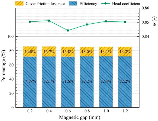
Figure 7.
Energy conversion and loss characteristics under different magnetic gaps.
To investigate the internal composition and physical mechanisms of disk friction loss, Table 2 quantifies the total loss power and its specific components for different magnetic gap configurations. The trend of the total disk friction loss power perfectly matches the loss rate shown in Figure 7. For magnetic gaps in the range of 0.8 to 1.2 mm, the disk friction loss power is relatively small, and the total loss power is minimized at 39.5 W when the gap is 0.8 mm. However, when the magnetic gap is reduced to 0.2 mm, the total loss power increases significantly to 43.1 W, an approximate increase of 9.1%. This confirms that the smaller the axial gap, the larger the absolute energy loss. Notably, disk friction loss is primarily composed of two parts: losses from the front and rear shrouds and the rotor. However, the sensitivity of these two components to the axial gap is distinctly different. The friction loss power from the front cover plate consistently fluctuates within a narrow range of 3.5 W to 4.1 W, being largely unaffected by variations in the gap. In contrast, the friction loss from the rear shroud and rotor exhibits high sensitivity to the axial gap. Its loss power surges from a minimum of 36.0 W at a 0.8 mm gap to a maximum of 39.2 W at a 0.2 mm gap, a substantial increase of 8.9%. This result demonstrates that the significant variation in the total disk friction loss is almost entirely driven by the rear cover plate and rotor component. A narrow fluid channel is formed between the rear cover plate and the pump casing. When the axial gap decreases, the fluid velocity gradient within this channel increases sharply, leading to significantly enhanced viscous shear. This, in turn, generates greater frictional torque and power loss. In summary, it is the sharp variation in friction loss at the rear shroud that dominates the overall loss profile and dictates the trend of the efficiency curve. Consequently, the 0.8 to 1.0 mm gap range emerges as the ideal interval for design optimization, as it provides the best balance between low friction loss and high operating efficiency.
Table 2.
Disk friction loss under different magnetic gaps.
4.2. Analysis of Pressure
The distributions of pressure, velocity, vorticity, and entropy production presented in Figure 8, Figure 9, Figure 10, Figure 11, Figure 12, Figure 13, Figure 14 and Figure 15 are visualized using ANSYS CFX Post based on the numerical simulation results from ANSYS CFX 2020. Figure 8 shows pressure distribution on the mid-section of the axial gap under different magnetic gaps. To facilitate comparison and analysis, the dimensionless pressure (p*) is defined as
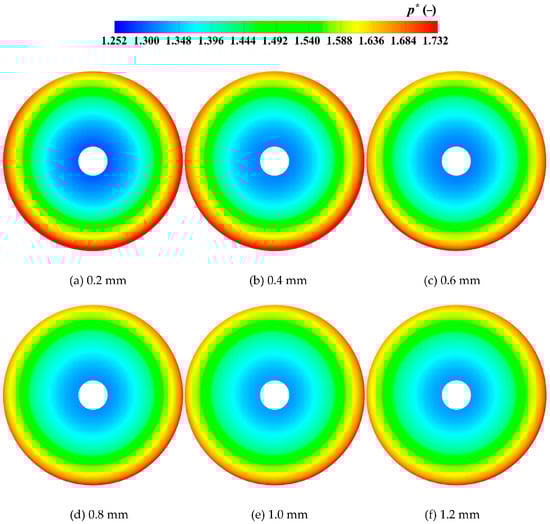
Figure 8.
Pressure distribution on the mid-section of the gap under different magnetic gaps. Here, p* denotes dimensionless pressure.
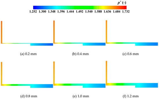
Figure 9.
Pressure distribution on the axial section of the gap under different magnetic gaps. Here, p* denotes dimensionless pressure.
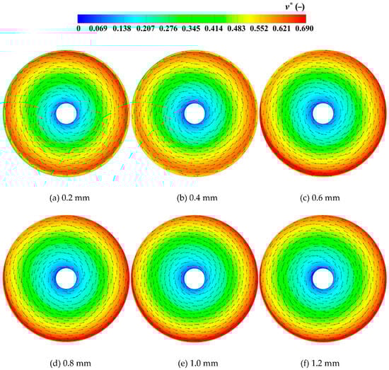
Figure 10.
Velocity distribution on the mid-section of the gap under different magnetic gaps. Here, v* denotes dimensionless velocity.
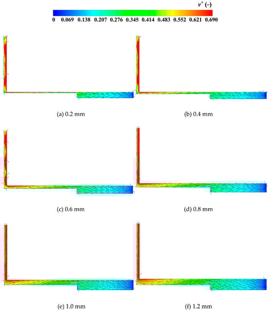
Figure 11.
Velocity distribution on the axial section of the gap under different magnetic gaps. Here, v* denotes dimensionless velocity.
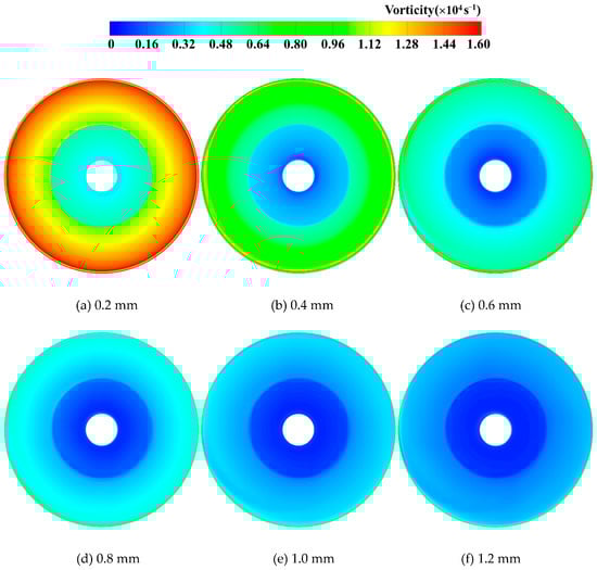
Figure 12.
Vorticity distribution on the mid-section of the gap under different magnetic gaps.
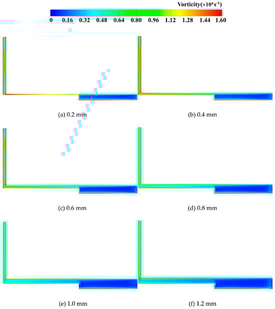
Figure 13.
Vorticity distribution on the axial section of the gap under different magnetic gaps.
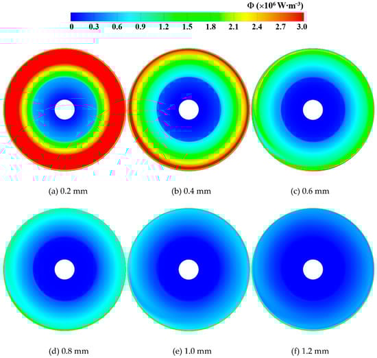
Figure 14.
Entropy production on the mid-section of the gap under different magnetic gaps.
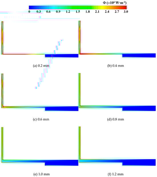
Figure 15.
Entropy production on the axial section of the gap under different magnetic gaps.
In all cases, due to centrifugal force, the fluid exhibits a pressure distribution where pressure increases with radius. This results in the formation of a distinct high-pressure ring in the region of the outer edge of the impeller. The morphology of this high-pressure ring is highly sensitive to changes in the axial gap, and its evolution process can be divided into two stages. In the magnetic gap range from 0.2 mm to 0.6 mm, the radial extent of the high-pressure ring shrinks significantly as the gap widens. This is mainly because viscous effects are dominant within this narrow flow channel, where intense viscous shear drastically dissipates the momentum of the fluid. When the magnetic gap widens into the 0.8 mm to 1.2 mm range, viscous effects are relatively weakened, allowing the inertial and centrifugal forces of the fluid to become the dominant factors. Consequently, the morphology of the high-pressure ring becomes more constrained by the geometric boundaries. Its radial contraction trend slows significantly, and the overall distribution tends to stabilize. Additionally, a distinct zone of reduced pressure appears on the high-pressure ring near the diffuser inlet (specifically, around the tongue or cutwater). This phenomenon is caused by flow separation and abrupt geometric changes. The circumferential extent of this weakened zone expands as the gap increases. The rate of this expansion follows a similar pattern; it is more rapid within the small gap range and tends to level off as the gap widens.
Figure 9 shows the pressure distribution on the axial cross-section below the tongue for different magnetic gaps. In the gap region between the rotor and the pump casing, the overall pressure level decreases significantly as the axial gap increases. In contrast to the decreasing pressure trend in the gap region, the pressure in the inner, smaller-radius region increases significantly as the axial gap expands. This is because a larger axial gap provides a longer axial interaction distance for the high-velocity fluid exiting the impeller, allowing for a more complete and efficient conversion of kinetic energy to static pressure. Compared to Figure 8, the pressure variation is also range-dependent. Whether considering the pressure decrease in the gap or the pressure increase in the inner region, the rate of change is more drastic in the small gap range of 0.2 to 0.6 mm, whereas it slows down significantly in the large gap range of 0.8 to 1.2 mm.
4.3. Analysis of Velocity
Figure 10 shows the velocity on the mid-section of the axial gap for different magnetic gaps. To facilitate comparison and analysis, the dimensionless velocity (v*) is defined as
In general, the velocity distribution for all configurations shows a trend of increasing with radius. In the small gap range from 0.2 to 0.6 mm, a distinct ring of relatively low velocity forms in the outermost circumferential region. This formation is attributed to the viscous effects of the wall. Notably, the width of this low-velocity band narrows significantly as the gap increases from 0.2 mm to 0.6 mm. For the 0.4 mm operating condition (Figure 10b), the intensity and extent of the main high-velocity region are distinctly reduced compared to the other cases. This observation is consistent with the previous analysis, showing a fluctuation in performance at this point. When the gap expands into the large range from 0.8 to 1.2 mm, the velocity distribution becomes highly consistent and is almost unaffected by further changes in the gap. A stable, high-velocity annular zone with a well-defined boundary is formed at the circumferential periphery.
However, to understand the more complex three-dimensional flow phenomena within the gap, such as secondary flow and flow separation, an in-depth analysis of the axial cross-section is necessary. Figure 11 shows the velocity on the axial cross-section below the tongue for different magnetic gaps. In the small gap range from 0.2 to 0.6 mm, a localized low-velocity core region forms within the gap between the rotor and the pump casing, particularly near the casing wall. The velocity in this region exhibits significant and disordered deflection and even reverse flow. This provides evidence of strong secondary flow and flow separation. This may be the primary source of energy dissipation and the direct cause of the poor performance. When the axial gap expands to the 0.8 to 1.2 mm range, the fluid throughout the entire gap maintains a relatively high velocity. The velocity exhibits a high degree of order, with all vectors consistently pointing in the radially outward direction. This indicates that secondary flow is effectively suppressed and flow separation has been eliminated.
4.4. Analysis of Vortex Distribution
Figure 12 shows the vorticity distribution on the mid-section of the gap for different magnetic gaps. The vorticity is primarily concentrated near the inner and outer radial boundaries, exhibiting a distinct annular distribution, while the vorticity in the central core region is relatively low. In the small gap range from 0.2 to 0.6 mm, the overall vorticity intensity of the flow field is extremely high. For the 0.2 mm gap, the predominance of high vorticity across most of the space demonstrates that the entire flow field is under intense viscous shear. As the gap increases to 0.6 mm, the high-vorticity region rapidly weakens and contracts, signifying a sharp decay in shear intensity. When the gap expands into the large range from 0.8 to 1.2 mm, the flow field transitions into a state of low vorticity and high stability. In this regime, the spatial structure of the vorticity distribution shows almost no further change and remains at a low overall level. This indicates that, at these larger gaps, the fluid’s velocity gradient has become much gentler. Inertial forces have superseded viscous shear as the dominant factor, leading the flow field into a stable and smooth state.
Figure 13 shows the vorticity distribution on the axial cross-section below the tongue for different magnetic gaps. In the small gap range from 0.2 to 0.6 mm, high-intensity vorticity is clearly attached to the surfaces of the rotor and the pump casing. This visually demonstrates that strong shear is generated within the boundary layer at the solid–fluid interface. The narrow flow channel causes these high-intensity shear layers from the opposing walls to nearly fill the entire gap, resulting in extremely high flow losses. This also explains the high disk friction loss in this range, as previously analyzed. When the gap expands to the 0.8 to 1.2 mm range, the high-vorticity layer attached to the walls becomes very thin, and its intensity is significantly weakened. More importantly, a vast low-vorticity core region appears between the rotor and the pump casing wall.
4.5. Analysis of Entropy Production
In pumps, due to the viscosity of the transported medium and the presence of Reynolds stresses during operation, mechanical energy is irreversibly converted into internal energy, leading to energy losses. According to the second law of thermodynamics, once the energy conversion process begins, entropy production is always positive because energy dissipation cannot be ignored [35,36,37]. The entropy production method is an effective tool for investigating the distribution and magnitude of energy losses within pumps, providing deeper insights into unsteady flow characteristics from the perspective of energy dissipation. A specific method for calculating entropy generation has been developed within the RANS framework, as shown in Equations (9)–(11).
where is the viscous dissipation, is the turbulent dissipation, ε is the dissipation rate of turbulent kinetic energy, and is the dissipation.
Figure 14 shows the entropy production distribution on the middle cross-section of the axial gap for different magnetic gaps. Overall, the widening of the magnetic gap has a significant regulatory effect on the energy dissipation characteristics within the rotor gap. As the gap increases from 0.2 mm to 1.2 mm, the overall entropy production in the flow field shows a decaying trend. The high entropy production region gradually recedes from a domain-wide distribution to become a localized, dissipation-sensitive zone near the walls. In the small gap range from 0.2 to 0.6 mm, the flow field is characterized by high dissipation and low efficiency. Especially in the 0.2 mm case, high entropy production fills nearly the entire flow channel, indicating that intense energy loss is widespread throughout the domain. As the gap increases to 0.6 mm, the high entropy production zone rapidly contracts and its intensity weakens, signifying that the overall energy dissipation level is quickly decreasing. When the gap expands into the large range from 0.8 to 1.2 mm, the flow field transitions to a low-dissipation, high-efficiency mode. The core flow region exhibits lower entropy production, and the high entropy production areas are confined to the wall boundary layers. This indicates that energy transport in the main flow region has become extremely efficient.
Figure 15 shows the entropy production distribution on the axial cross-section below the pump tongue for different magnetic gaps. In the small gap range from 0.2 to 0.6 mm, high entropy production adheres to all wall surfaces of the rotor and the pump casing. This visually demonstrates that the root cause of high disk friction loss under small gaps is precisely the intense viscous dissipation within these wall boundary layers. At the same time, the regions of secondary flow and flow separation observed previously in Section 4.3 are also concentrated zones of entropy production from turbulent dissipation; these two factors combine to form the main energy loss for this operating condition. When the gap expands to the 0.8 to 1.2 mm range, the wall-attached layer of high entropy production becomes extremely thin, and its intensity is significantly weakened. More importantly, the vast core fluid region between the walls of the rotor and the pump casing exhibits extremely low entropy production. This indicates that, with the optimization of the flow structure, irreversible energy loss is largely confined to the thin boundary layers, thereby achieving efficient energy transport.
4.6. Analysis of Pressure Fluctuations
4.6.1. Monitoring Point Locations
The magnetic gap is one of the key parameters for submersible axial motors, and its operating conditions significantly influence performance and stability. Therefore, analyzing pressure fluctuations is of critical importance [38]. Figure 16 illustrates the locations of the monitoring points. Eight stationary monitoring points, labeled AP1 to AP8, are arranged in the rear chamber along the circumferential direction at 45-degree intervals. These points are situated on Plane 1 to capture pressure fluctuations in the magnetic gap between the rotor and stator. Plane 1 is the mid-section of the magnetic gap, with the distance from either the rotor or the stator wall being equal to 0.5 times the total magnetic gap distance.
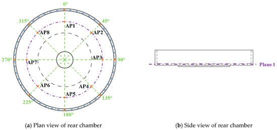
Figure 16.
Monitoring locations.
The non-dimensional pressure coefficient Cp denotes as:
where pi is the transient pressure and represents the mean pressure recorded at the monitoring point over one cycle.
For this test pump, the impeller rotating frequency is 86.67 Hz. The horizontal axis (t*) of the pressure fluctuations time-domain plot represents the ratio of the specific time to the impeller rotation cycle. The horizontal axis (f*) of the pressure fluctuations frequency-domain plot is a dimensionless frequency, defined as the ratio of the monitored frequency to the impeller rotating frequency. Thus, f* represents a multiple of the impeller rotating frequency.
4.6.2. Pressure Fluctuations in Rear Chamber
The time-domain and frequency-domain plots of pressure fluctuations (Figure 17 and Figure 18) are obtained by extracting transient pressure data from ANSYS CFX 2020 numerical simulations and subsequently analyzed and plotted using Origin 2021b software, including Fourier transform methods. Figure 17 shows the time-domain plots of pressure fluctuations at each monitoring point for different magnetic gaps. The vertical axis represents the pressure fluctuation coefficient, Cp, which is a dimensionless quantity representing the normalized pressure fluctuations. The horizontal axis represents the dimensionless time, t* = t/T, where t is the actual time and T is a characteristic revolution period. All curves exhibit a periodicity that corresponds to the number of blades, and this periodic characteristic does not vary with the magnetic gap. This indicates that the excitation mechanism for pressure fluctuations is primarily dominated by the blade passing frequency. When the magnetic gap is 0.2 mm, the pressure fluctuation amplitude at AP6 is the smallest. As the magnetic gap increases to the range of 0.4 to 1.0 mm, the minimum amplitude shifts to AP5. When the magnetic gap is further increased to 1.2 mm, the minimum amplitude is found at AP4.
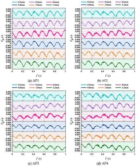
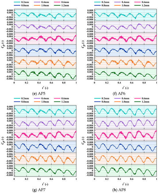
Figure 17.
Time domain of pressure fluctuations at AP1 to AP8 under different magnetic gaps. Here, t* denotes dimensionless time.
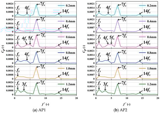
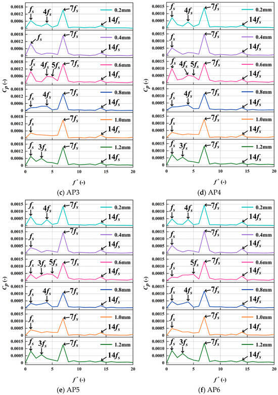
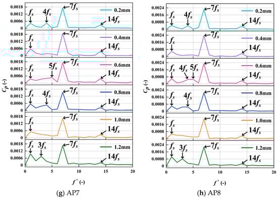
Figure 18.
Frequency domain of pressure fluctuations at AP1 to AP8 under different magnetic gaps. Here, f* denotes dimensionless frequency.
Notably, AP8, located below the tongue, has the largest pressure fluctuation amplitude at a gap of 0.4 mm, whereas AP1, located below the diffuser inlet, consistently exhibits the maximum amplitude under all other magnetic gaps. This difference indicates that the region near AP1 is a high-risk zone for fluctuation under all magnetic gaps. When the magnetic gap is 1.2 mm, the absolute difference between the maximum and minimum pressure fluctuation amplitudes reaches its peak. However, at the magnetic gap of 0.8 mm, the relative increase in the maximum amplitude compared to the minimum is the highest, reaching 57.4%.
For all magnetic gaps, the average intensity of pressure fluctuation is lowest, located below the middle transition area of the volute diffusion section. In contrast, the average intensity at monitoring point AP1, located below the diffuser inlet, is the highest, reaching a maximum of 1.9 times the value at AP5. As the magnetic gap increases from 0.2 mm to 1.2 mm, the average fluctuation intensity at AP5 shows a trend of decreasing and then increasing, reaching a minimum at the gap of 0.8 mm. Conversely, the average fluctuation intensities at AP1 and AP8 continuously increase as the gap widens, reaching their respective peak values at 1.2 mm. The data indicates that, at the magnetic gap of 0.8 mm, the average intensity of pressure fluctuation is minimum. This represents a 19.3% reduction compared to the maximum average intensity observed at the gap of 0.6 mm.
Figure 18 displays the frequency-domain plots of pressure fluctuations at each monitoring point (AP1 to AP8) for different magnetic gaps. The time-domain plots of pressure fluctuations are obtained by extracting transient pressure data from ANSYS CFX 2020 numerical simulations and subsequently analyzed and plotted using Origin 2021 software. The vertical axis represents the pressure fluctuation coefficient, Cp, a dimensionless quantity representing the normalized pressure fluctuations. The horizontal axis represents the dimensionless frequency, f* = f/fs, where f is the actual frequency and fs is the rotation frequency. At all magnetic gaps, the dominant frequency of the pressure fluctuations is the blade frequency (7fs). This is accompanied by components at the rotation frequency (fs) and the second harmonic of the blade frequency (14 fs), but their amplitudes are significantly lower than that of the dominant frequency. The regions of AP1, AP3, AP4, and AP8 are identified as sensitive to the rotation frequency. At the magnetic gaps of 0.4 mm and 0.6 mm, the rotation frequency amplitudes at AP3 and AP4 reach their respective peaks, being 42% to 68% higher than at other monitoring points. When the magnetic gap increases to 1.2 mm, the rotation frequency amplitudes at AP1 and AP8 surge to their maximum, representing increases of 95.6% and 78.2%, respectively, compared to the gap of 0.8 mm. When the magnetic gap is 0.8 mm, the blade frequency amplitudes at AP4 and AP5 reach their minimum values. This is a reduction of 23.0% and 26.4%, respectively, compared to their maximum values observed at the 0.4 mm gap. This indicates that, at these magnetic gaps, the disturbance in this region caused by the periodic sweep of the blades can be effectively suppressed.
For all magnetic gaps, the blade frequency amplitudes at AP1 and AP8 are significantly higher than at other monitoring points. These amplitudes both reach their peak values at a gap of 0.4 mm, representing increases of 9.7% and 12.9%, respectively, compared to their minimum values at the gap of 0.8 mm. The pressure fluctuation spectrum also reveals other harmonic components that vary with the gap. When the magnetic gap is 0.2 mm and 1.2 mm, discrete harmonic components appear at 4 times the rotation frequency (4fs) and 3 times the rotation frequency (3fs), respectively, with amplitudes second only to that of the rotation frequency. At the magnetic gap of 0.6 mm, broadband harmonic influences at 4fs and 5fs are observed. Furthermore, at points AP5 to AP7, an increase in the amplitude of the 3fs component forms an enhanced broadband harmonic zone. When the magnetic gap is 0.8 mm, the range of harmonic influence expands into a continuous broadband zone from the rotation frequency to 4 fs, though with a reduced energy density. As the magnetic gap further increases to 1.0 mm, the harmonic energy in this continuous broadband zone decays even more.
5. Conclusions
This paper systematically studies the nonlinear effects of the magnetic gaps on the energy performance, flow characteristics, and pressure fluctuations of axial-flux canned motor pumps. The main conclusions are as follows:
- The energy performance exhibits a significant non-linear response, with different optimal gaps for different performance indicators. The head coefficient peaks at a 0.4 mm gap, while maximum efficiency occurs at 1.0 mm. For a 0.2 mm magnetic gap, strong viscous shear effects in the confined space dominate, causing disk friction power loss to surge by nearly 10% and severely undermining efficiency. Notably, disk friction loss reaches its minimum at the 0.8 mm magnetic gap, indicating an optimal magnetic gap that balances shear and leakage effects. This finding provides crucial practical guidance for optimizing the hydraulic design of axial flux canned motor pumps.
- Both the pressure distribution and fluctuation intensity are highly sensitive to the magnetic gaps. For small gaps (0.2–0.6 mm), viscous dissipation dominates, causing the circumferential high-pressure ring to contract radially. For the magnetic gap of 0.8 mm to 1.2 mm, the effect of mainstream inertial forces becomes prominent, and the high-pressure zone tends to stabilize. The Blade Passing Frequency is the dominant frequency, with high fluctuations concentrated near the tongue and the diffuser inlet. For the 0.8 mm magnetic gap, the pressure fluctuation amplitude is lowest.
- The internal flow reflects the competitive mechanism between viscous and inertial forces. For small magnetic gaps (0.2–0.6 mm), strong shear action forms a continuous low-velocity, high-vorticity band at the circumferential periphery and induces secondary flows at abrupt geometric changes, leading to flow disorder. For the magnetic gap of 0.8 mm to 1.2 mm, mainstream inertial forces gradually dominate, causing the flow pattern to become more ordered. The high-velocity annular zone remains stable, and the vorticity accumulation near the rotor and casing walls is significantly weakened.
- Enlarging the magnetic gap attenuates viscosity-dominated momentum dissipation, thereby significantly reducing the entropy production. For small magnetic gaps (0.2–0.6 mm), the synergistic effect of strong viscous shear and geometric discontinuities forms a high entropy production zone. For the magnetic gap of 0.8 mm to 1.2 mm, viscosity-dominated momentum dissipation is effectively suppressed. The primary region of energy loss degenerates into a localized, near-wall dissipation band, while the mainstream region exhibits efficient, low-dissipation transport characteristics. This perfectly corresponds with the macroscopic phenomenon of higher efficiency observed at larger magnetic gaps.
While this study identifies the hydraulically optimal magnetic gap, it is acknowledged that practical engineering considerations such as manufacturing tolerances, thermal expansion, and long-term wear are crucial for real-world applications. Therefore, future work will involve coupled thermal–structural–fluid multiphysics analysis, integrating structural mechanics and materials science, to ensure the feasibility and reliability of the design under actual operating conditions and to guide comprehensive multi-objective optimization.
Author Contributions
Conceptualization, Q.Z. and Y.G.; methodology, Q.Z. and Y.G.; software, J.B.; validation, Q.Z. and J.B.; formal analysis, Q.Z.; investigation, Q.Z. and J.B.; resources, Y.G.; data curation, Q.Z.; writing—original draft preparation, Q.Z.; writing—review and editing, Q.Z. and Y.G.; visualization, Q.Z. and J.B.; supervision, Y.G. and J.B.; project administration, Y.G.; funding acquisition, Y.G. All authors have read and agreed to the published version of the manuscript.
Funding
This work was supported by the National Natural Science Foundation of China (grant number 52206055) and the Priority Academic Program Development of Jiangsu Higher Education Institutions (PAPD).
Data Availability Statement
The raw data supporting the conclusions of this article will be made available by the authors on request.
Conflicts of Interest
The authors declare no conflicts of interest.
Nomenclature
The following nomenclature are used in this manuscript:
| Symbols | |
| b2 | Blade outlet width, mm |
| b3 | Volute inlet width, mm |
| Cp | Dimensionless pressure coefficient |
| D1 | Blade inlet diameter, mm |
| D2 | Blade outlet diameter, mm |
| D3 | Volute inlet diameter, mm |
| Dd | Volute outlet diameter, mm |
| Dr | Motor rotor diameter, mm |
| fi | External force, N/m3 |
| fs | Shaft frequency, Hz |
| f* | Dimensionless frequency |
| g | Gravitational acceleration, m/s2 |
| H | Head for pumps, m |
| Lr | Motor rotor axial width |
| n | Rotating speed of impeller, rpm |
| p | Pressure, Pa |
| pout | Static pressures at the outlet, Pa |
| pin | Static pressures at the inlet, Pa |
| pi | Prompt pressure, Pa |
| Average pressure, Pa | |
| p* | Dimensionless pressure |
| P | Shaft power, W |
| Q | Flow rate for pumps, L/min |
| Qd | Design flow rate for pumps, L/min |
| Q* | Dimensionless flow rate |
| t | Time, s |
| t* | Dimensionless time |
| T | Shaft torque, N·m |
| T0 | Unloaded shaft torque, N·m |
| u2 | Circumferential velocity at blade outlet, m/s |
| v* | Dimensionless velocity |
| x | Cartesian coordinates |
| Zb | Number of blades |
| β1 | Blade inlet angle, ° |
| β2 | Blade outlet angle, ° |
| ΔZ | Vertical distance between the inlet and outlet pressure sensors, m |
| η | Efficiency, % |
| μ | Viscosity, kg/(m·s) |
| ρ | Density, kg/m3 |
| Dissipation, W/m3 | |
| Viscous dissipation, W/m3 | |
| Turbulent dissipation, W/m3 | |
| φ0 | Tongue angle, ° |
| Reynolds stress tensor | |
| Subscripts | |
| i | Free index |
| j, k | Dummy index |
| Abbreviations | |
| CFD | Computational Fluid Dynamics |
| Exp. | Experimental |
| GCI | Grid Convergence Index |
| Num. | Numerical |
| RANS | Reynolds-Averaged Navier–Stokes |
| SST | Shear Stress Transport |
References
- Gu, Y.; Yang, A.; Bian, J.; Shariff, A.M.; Stephen, C.; Wang, Q.; Cheng, L. Investigation of energy performance and unsteady flow characteristics of a multi-stage centrifugal pump under various seal wear conditions for renewable energy pumping systems. Renew. Energy 2025, 256, 123998. [Google Scholar] [CrossRef]
- Si, Q.; Xu, H.; Deng, F.; Xia, X.; Ma, W.; Guo, Y.; Wang, P. Study on performance improvement of low specific speed multistage pumps by applying full channel hydraulic optimization. J. Energy Storage 2024, 99, 113238. [Google Scholar] [CrossRef]
- Shi, Z.; Sun, X.; Yang, Z.; Cai, Y.; Lei, G.; Zhu, J.; Lee, C.H.T. Design Optimization of a Spoke-Type Axial-Flux PM Machine for In-Wheel Drive Operation. IEEE Trans. Transp. Electrif. 2024, 10, 3770–3781. [Google Scholar] [CrossRef]
- Zhu, X.; El Shahat, S.A.; Lai, F.; Jiang, W.; Li, G. Numerical investigation of rotor–stator interaction for canned motor pump under partial load condition. Mod. Phys. Lett. B 2020, 34, 2050039. [Google Scholar] [CrossRef]
- Tinni, A.; Knittel, D.; Nouari, M.; Sturtzer, G. Electrical–thermal modeling of a double-canned induction motor for electrical performance analysis and motor lifetime determination. Electr. Eng. 2021, 103, 103–114. [Google Scholar] [CrossRef]
- Huang, Y.; Jiang, L.; Ni, Y.; Lei, H.; Gao, G. Control method analysis with high performance and stability for permanent magnet motor based on canned structure. Int. J. Electr. Power Energy Syst. 2022, 143, 108441. [Google Scholar] [CrossRef]
- Zhou, G.H.; Qiao, M.Z.; Wu, D.; Hao, Q.; Zhang, X.; Shi, P.; Tan, B. Low Noise Optimization Design of Integrated Permanent Magnet Synchronous Motor Based on Multi-Physical Field Coupling. IEEE Trans. Appl. Supercond. 2024, 34, 5207004. [Google Scholar] [CrossRef]
- Kanyolo, T.N.; Oyando, H.C.; Chang, C. Acceleration Analysis of Canned Motors for SMR Coolant Pumps. Energies 2023, 16, 5733. [Google Scholar] [CrossRef]
- Pang, D.-C.; Wang, C.-T. A Wireless-Driven, Micro, Axial-Flux, Single-Phase Switched Reluctance Motor. Energies 2018, 11, 2772. [Google Scholar] [CrossRef]
- Eker, M.; Zöhra, B.; Akar, M. Experimental performance verification of radial and axial flux line start permanent magnet synchronous motors. Electr. Eng. 2024, 106, 1693–1704. [Google Scholar] [CrossRef]
- Ai, L.; Ma, P.; Miao, S.; Jiang, S.; Xu, X. Modelling and analysis of a superconducting magnetic coupler used for cryogenic pump. IET Electr. Power Appl. 2024, 18, 1131–1141. [Google Scholar] [CrossRef]
- Ai, L.; Zhang, G.; Jing, L.; Xu, X.; Si, J. Behaviors of Axial and Radial Electromagnetic Force for Cryogenic Disk Motor. IEEE Trans. Energy Convers. 2021, 36, 874–882. [Google Scholar] [CrossRef]
- Ai, L.; Zhang, G.; Li, W.; Liu, G.; Song, N.; Xiao, L.; Lin, L. Research on a Superconducting Magnetic Bearing System for Submerged Cryogenic Disk Motor-Pump. IEEE Trans. Appl. Supercond. 2018, 28, 5202505. [Google Scholar] [CrossRef]
- Gadiyar, N.; Bohach, G.; Nahin, M.M.; Van de Ven, J.; Severson, E.L. Development of an Integrated Electro-Hydraulic Machine to Electrify Off-highway Vehicles. IEEE Trans. Ind. Appl. 2022, 58, 6163–6174. [Google Scholar] [CrossRef]
- Zhang, Y.; Li, J.; Yan, W.; Chng, C.-B.; Chui, C.-K.; Yang, X.; Zhao, S. Advancing energy efficiency in electric vehicles: Design and performance analysis of innovative axial-flux PM motor-driven coolant pumps. Energy 2024, 313, 134112. [Google Scholar] [CrossRef]
- Fan, R.; Liang, Z.; Fan, B.; Chen, S.; Lv, W.; Xu, W.; Zheng, J.; Wang, D. Numerical analysis of internal flow characteristics and energy consumption assessment in full flow field of multi-stage centrifugal pump considering clearance flow. Adv. Mech. Eng. 2022, 14, 16878132221123423. [Google Scholar] [CrossRef]
- Gu, Y.; Bian, J.; Wang, C.; Sun, H.; Wang, M.; Ge, J. Transient numerical investigation on hydraulic performance and flow field of multi-stage centrifugal pump with floating impellers under sealing gasket damage condition. Phys. Fluids 2023, 35, 107123. [Google Scholar] [CrossRef]
- Zhan, P.; Wei, L.; Liu, R.; Liang, M.; Qiang, Y. Flow Field Modeling and Simulation of High-Speed Gear Pump Considering Optimal Radial and End Clearance. IEEE Access 2023, 11, 64725–64737. [Google Scholar] [CrossRef]
- Hou, X.; Cheng, Y.; Yang, Z.; Liu, K.; Zhang, X.; Liu, D. Influence of Clearance Flow on Dynamic Hydraulic Forces of Pump-Turbine during Runaway Transient Process. Energies 2021, 14, 2830. [Google Scholar] [CrossRef]
- Zheng, L.; Chen, X.; Qu, J.; Ma, X. A Review of Pressure Fluctuations in Centrifugal Pumps without or with Clearance Flow. Processes 2023, 11, 856. [Google Scholar] [CrossRef]
- Guang, W.-L.; Liu, Q.; Jin, F.-Y.; Tao, R.; Xiao, R.-F. Analysis of clearance flow of a fuel pump based on dynamical mode decomposition. J. Hydrodyn. 2024, 36, 781–795. [Google Scholar] [CrossRef]
- Li, Q.; Li, S.; Wu, P.; Huang, B.; Wu, D. Investigation on Reduction of Pressure Fluctuation for a Double-Suction Centrifugal Pump. Chin. J. Mech. Eng. 2021, 34, 12. [Google Scholar] [CrossRef]
- Liang, S.; Pang, S.; Liu, J.; Chen, Z.; Sun, D.; Li, C. Unsteady internal flow characteristics study of a hydrogen circulation pump under different pressure differential conditions. Int. J. Hydrogen Energy 2024, 60, 1147–1156. [Google Scholar] [CrossRef]
- Li, L.; Yan, D.; Liu, X.; Zhao, W.; Wang, Y.; Pang, J.; Wang, Z. Numerical Study on the Effect of Crown Clearance Thickness on High-Head Pump Turbines. Water 2023, 15, 3397. [Google Scholar] [CrossRef]
- Li, Y.; Zheng, Y.; Meng, F.; Wang, M.; Li, Y. Numerical simulation on the influence of root clearance on the hydraulic performance of axial flow pump device. J. Braz. Soc. Mech. Sci. Eng. 2022, 44, 161. [Google Scholar] [CrossRef]
- Zhou, L.; Zhou, C.; Bai, L.; Agarwal, R. Numerical and Experimental Analysis of Vortex Pump with Various Axial Clearances. Water 2024, 16, 1602. [Google Scholar] [CrossRef]
- Jia, X.; Yu, Y.; Li, B.; Wang, F.; Zhu, Z. Effects of incident angle of sealing ring clearance on internal flow and cavitation of centrifugal pump. Proc. Inst. Mech. Eng. Part E J. Process Mech. Eng. 2024, 238, 2867–2882. [Google Scholar] [CrossRef]
- Oro, J.F.; Perotti, R.B.; Vega, M.G.; González, J. Effect of the radial gap size on the deterministic flow in a centrifugal pump due to impeller-tongue interactions. Energy 2023, 278, 127820. [Google Scholar] [CrossRef]
- Liu, J.; Xi, W.; Lu, W. Optimization Design of Radial Clearance between Stator and Rotor of Full Cross-Flow Pump Units. J. Mar. Sci. Eng. 2024, 12, 1124. [Google Scholar] [CrossRef]
- Gu, Y.; Zhu, Q.; Bian, J.; Wang, Q.; Cheng, L. Novel sealing design for high-speed coolant pumps: Impact on energy performance, axial thrust and flow field. Energy 2025, 321, 135511. [Google Scholar] [CrossRef]
- Chang, H.; Yang, J.; Wang, Z.; Peng, G.; Lin, R.; Lou, Y.; Shi, W.; Zhou, L. Efficiency optimization of energy storage centrifugal pump by using energy balance equation and non-dominated sorting genetic algorithms-II. J. Energy Storage 2025, 114, 115817. [Google Scholar] [CrossRef]
- Huang, X.; Jin, G.; Guo, Q.; Liu, X.; Lu, J. A method for evaluating the effect induced by vortices on the moment and efficiency of the fluid machinery. Phys. Fluids 2024, 36, 115165. [Google Scholar] [CrossRef]
- Wang, D.; Gu, Y.; Stephen, C.; Ji, Q. Blade number effects on performance and internal flow dynamics in high-speed coolant pumps. Phys. Fluids 2025, 37, 015240. [Google Scholar] [CrossRef]
- Wang, C.; Zhang, S.; Zhang, T.; Zhang, H.; Li, M. Study of a Companion Trajectory Kinematics Analysis Method for the Five-Blade Rotor Swing Scraper Pump. Machines 2024, 12, 877. [Google Scholar] [CrossRef]
- Wang, H.; Wu, X.; Xu, X.; Bian, S.; Meng, F. Size Effect on Energy Characteristics of Axial Flow Pump Based on Entropy Production Theory. Machines 2025, 13, 252. [Google Scholar] [CrossRef]
- Wang, T.; Yu, H.; Xiang, R.; Chen, X.; Zhang, X. Performance and unsteady flow characteristic of forward-curved impeller with different blade inlet swept angles in a pump as turbine. Energy 2023, 282, 128890. [Google Scholar] [CrossRef]
- Ji, L.; Li, W.; Shi, W.; Chang, H.; Yang, Z. Energy characteristics of mixed-flow pump under different tip clearances based on entropy production analysis. Energy 2020, 199, 117447. [Google Scholar] [CrossRef]
- Gu, Y.; Bian, J.; Wang, Q.; Stephen, C.; Liu, B.; Cheng, L. Energy performance and pressure fluctuation in multi-stage centrifugal pump with floating impellers under various axial oscillation frequencies. Energy 2024, 307, 132691. [Google Scholar] [CrossRef]


Disclaimer/Publisher’s Note: The statements, opinions and data contained in all publications are solely those of the individual author(s) and contributor(s) and not of MDPI and/or the editor(s). MDPI and/or the editor(s) disclaim responsibility for any injury to people or property resulting from any ideas, methods, instructions or products referred to in the content. |
© 2025 by the authors. Licensee MDPI, Basel, Switzerland. This article is an open access article distributed under the terms and conditions of the Creative Commons Attribution (CC BY) license (https://creativecommons.org/licenses/by/4.0/).