Abstract
A condition-based monitoring (CBM) system provides the possibility for the railway industry to guarantee reliability by executing prompt and low-cost maintenance. In this study, a simple model-based condition monitoring strategy for the railway vehicle suspension system is demonstrated. The method is based on a recursive least-square (RLS) algorithm regarding a deterministic parametric model. The fault detection approach for the locomotive suspension system is illustrated with three diagnostic modules. Multi-body simulation data are employed to validate the feasibility of this CBM strategy. The designed diagnostic model reveals that the suspension parameter estimates are consistent with the reference values. The corresponding demonstrator provides evidence that the monitoring system has potential applications and is suitable for further development.
1. Background
1.1. Condition Monitoring of Railway Vehicle Suspension System
Modern railway transportation requires a comprehensive condition-based monitoring (CBM) system for the optimization of the rolling stock maintenance. A CBM system should be able to detect the in-service failures and contribute to prompt decision making for the operational conditions by providing diagnostic information regarding component degradation. Additionally, it should be feasible to execute reasonable maintenance activities to guarantee the performance of the vehicles and reduce life-cycle costs according to the information provided by CBM systems [1,2]. Since safety, reliability and cost efficiency are the priorities of the railway industry, the application of a CBM system for railway vehicles will be in considerable demand in the foreseeable future.
This study focuses on the condition monitoring of the railway vehicle suspension system. As one of the most critical components of the rail vehicle, the suspension system guarantees good ride performance by isolating and attenuating the vibration caused by the irregularity of the wheel/rail interface. In addition to supporting the weight of the vehicle, the suspension system is responsible for the steering in curves and the avoidance of hunting motion. Even though the suspension system is critical in the performance of the train, no mature condition monitoring technique has been applied in this field so far, which makes the maintenance of the numerous suspension components very expensive.
This work focuses on the condition monitoring of the suspension system based on the measurements obtained from a vibration sensor mounted on the vehicle. Unlike the conventional fault detection in the depot, this approach is aimed at the online identification of the impact of the suspension performance on operational conditions. The vehicle motion caused by the irregularity at the wheel/rail interface serves as a ‘natural exciter’ for the vehicle suspension component; this evidently contributes to the feasibility of this vehicle-based condition monitoring system.
According to the perspective of the utilization of the signal, the condition monitoring techniques can be categorized into two main types: model-based and data-driven approaches. However, it is not necessary to set a clear division between the model-based and the data-driven methods using a strict definition, since the model-based algorithm inevitably utilizes data-driven techniques in its identification procedures.
1.2. Pure Data-Driven Assessments
The main purpose of a pure data-driven method is to extract the principal information revealing the distinction between faulty and fault-free cases via the assessment of the response signal. In certain situations, the response signal itself contains certain information for the system diagnosis.
One data-driven method based on the Random Decrement Technique (RDT) and Prony method is utilized to isolate the faults in the lateral suspensions of a passenger vehicle [3]. In [4], the cross-correlation of acceleration signals at different locations on the bogie frame is used to indicate suspension faults. In [5], the detection of suspension damages is performed on the assessment of statistical parameter compliance with normative values using a three-dimensional diagnostic space. In [6], experimental data and the simulation results of acceleration values on four reference bogie points are used to detect a damper failure in the primary suspension with the comparisons of acceleration signals. In [7], an MSVR (multi-output support vector regression)-based supervised learning model is used to monitor the stiffness and damping coefficients of the suspension system with real-time measurement. In [8], the state health monitoring system of high-speed train suspension is proposed in the form of parameter approximation with a multibody simulation code and a Bayesian calibration approach. In [9], the ACS-SSI (average-correlation-signals-based stochastic subspace identification) algorithm is used in a condition monitoring scheme for the vehicle suspension via a modal identification method. In [10], the frequency response functions between accelerometer signals in vehicle are used as suspension fault indicators and fed into the classification algorithms in the machine learning procedure. In [11], a Bidirectional Long Short-Term Memory (BiLSTM) neural network is proposed for the fault detection of railway vehicle suspension.
One important condition in the application of a pure data-driven technique is that a meaningful difference for the abnormal situation needs to be identified effectively in comparison with the normal one. In fact, this task can be very difficult for the vehicle suspension system, because the differences in dynamic responses between the faulty and fault-free cases can be very small due to the system redundancy. This problem is also reflected in the frequency domain feature of the signal. In many cases, it is difficult to distinguish between the faulty and fault-free scenarios by analyzing their signals’ spectral energies, resonance peaks, etc. Meanwhile, the frequency feature of the vehicle is affected by different external disturbances, such as track irregularities. In the suspension system, the signal itself cannot directly reflect the health condition of the suspension component. In contrast, the relationship between signals needs to be taken into consideration in diagnostics.
1.3. Model-Based Assessments
Model-based techniques are equipped with the potential capacities to reveal the unknown parameters or states in quantitative forms. They are particularly preferable under the condition that the relationships between signals are known and accessible for the estimation of key parameters in the system. In the vehicle suspension system, as a fault occurs in a suspension component, there should be a certain parameter deviation in that component compared with the normal operational situation. In such a situation, the parameter estimation technique is preferred for the diagnosis of the suspension component with a quantitively method.
In this background, many model-based approaches are dedicated to the fault detection of the lateral vehicle suspensions. For instance, the Rao-Blackwellised Particle filter technique (RBPF) is applied to estimate the damping coefficients of lateral and yaw dampers and the wheel tread conicity of a passenger car [12]. The interacting multiple-model method (IMM) based on the Kalman filter is used to monitor faults occurring in the lateral and yaw dampers of the bogie [13]. In [14], the residuals generated from one Hybrid Extended Kalman filter are analyzed to isolate the faults occurring in lateral suspensions. In [15], a Cubature Kalman filter is proposed for the suspension fault diagnosis associated with a sensitivity analysis of a secondary vertical damper fault. However, these approaches, which are based on state-space models, are very complicated and only dedicated to certain suspension component faults. It is difficult to implement these works in realistic engineering problems. The mentioned methods are expected to identify the suspension faults by observing the states in the dynamic model. However, the observation of the state is not meaningful enough in this scenario, because the motion of the vehicle only represents its response under the external disturbance.
1.4. Aim of the Demonstrator
The demonstrator presented in this study constitutes a simple model-based strategy for monitoring the condition of suspension components in a locomotive bogie. The vehicle suspension is a coupled dynamic system, since the contributions of dampers and springs coexist in the vibration of the sprung mass. Considering the fault diagnosis of the suspension system, it is essential to apply an efficient tool to decouple the contribution of each suspension component.
As mentioned before, for a vehicle suspension system, the relationships between signals should be more important than the signals themselves. Realistically, the relationship between the motion of the suspension component and the acceleration of the sprung mass is determined. It suggests a more straightforward model-based approach for identifying the suspension parameter. In a linear system, the dynamic influence of the suspension component on a sprung mass can be described in a parametric form. With this approach, multiple suspension parameters could be estimated in parallel from a dynamic system, which is more suitable for the real engineering application.
2. Parametric Model and RLS Method
2.1. Parametric Model for Vehicle Dynamics
In a vehicle system, the acceleration response of the sprung mass for each time t is mainly determined by the corresponding sum of suspension loads. Its motion equation can be written in a simple algebraic form of Newton’s second law, which concentrates on the influence of the suspension component. For the translational motion equation, it is generally expressed as:
where Ms is the sprung mass, As represents the translational acceleration of the sprung mass. Ci represents the damping coefficient of damper i, Vi is the velocity for the damper i, Kj is the stiffness of spring j, Dj is the displacement for the spring j, and Fex represents the external load regarded as the modeling error.
For the rotational motion equation, it can be generally expressed as:
where αs represents the angular acceleration of the sprung mass, Is is the moment inertia of sprung mass. LCi represents the moment arm of damper i, LKj represents the moment arm of spring j. CTu is the damping coefficient of the torsional damper u, ωu is the torsional velocity for the torsional damper u, KTw is the stiffness of torsional spring w, θw is the torsional displacement for the torsional spring w, and Mex is the external moment reckoned as the model error.
The kinetic variables in Equations (1) and (2) can be measured directly or indirectly. Their relationships are determined by the motion equations. As the measured data at each time are independent of the others, the whole dataset can be considered as an over-determined equation set. In this sense, the identification of the suspension parameter can be transformed into a simple least-square (LS) problem. However, an LS cannot provide any meaningful estimates in this scenario, because the pseudo-inverse is seriously ill-conditioned and a single LS estimate is prone to be contaminated by the error. In contrast, the recursive least-square (RLS) algorithm can overcome these mathematical problems.
2.2. Recursive Least-Square Filtering
The fault detection algorithm utilizes the simple recursive least-square (RLS) filtering [16,17,18,19,20,21,22]. RLS is an adaptive time-domain filter, which is suitable for an on-line diagnostic system. RLS can estimate parameters within a noisy system with the correlation and memory properties. The memory features can significantly improve the effectiveness of parameter identification in the processing of the noisy vibration signals. It is believed that RLS is closely linked with Kalman filtering (KF). RLS can be regarded as a special case of KF, but with a dynamic observation. Furthermore, RLS is also an on-line ‘supervised’ machine learning technique, which is a subfield of artificial intelligence (AI).
RLS is dedicated to the deterministic parametric model. It has a very simple computational procedure:
Referring to the suspension model, for each iteration, the error e(1 × 1) is expressed with the previous parameter estimate:
where Y(t)(1×1) is the system output, i.e., the total inertia force/torque of the sprung mass, X(t)(n×1) is the regressor vector containing the velocities and displacements of the suspension components. These variables can be measured directly or indirectly. θ(t)(n×1) is the vector comprising the estimated suspension parameters.
A Kalman gain G(n×1) is introduced with a covariance matrix P(n×n):
where λ is a forgetting factor. When λ = 1, the ‘growing memory’ is used with all errors to be treated equally. This is very important for vibration signals, since the maximum information among signals needs to be extracted.
The current parameter estimate is updated with the Kalman gain and the current error,
The update of the new covariance matrix P(t) is expressed as:
The performance of RLS is almost insensitive to the initial conditions. In the usage of RLS, the initial value of the parameter vector θ0 can be set to zero. The initial value of covariance matrix P0 can be assigned as a diagonal matrix with large entries. θ(t) and P(t) will be automatically updated in each iteration of RLS algorithm. Due to the Kalman filtering feature, the RLS provides a stable and fast convergence in the parameter estimation.
3. Vehicle Dynamics Model of Demonstrator
Under this framework, a vehicle model of a heavy-duty Co-Co locomotive was used to illustrate the application of the proposed RLS-based condition monitoring strategy. This locomotive model represents a currently widely used type of locomotive with many linear suspension components, such as viscous dampers. The total mass of this heavy-duty six axle locomotive is 126 t. The bogie wheelbase of this locomotive is 4.2 m. A VAMPIRE® multi-body model of this vehicle is employed to generate ‘virtual measurements’ to demonstrate the newly developed condition monitoring scheme. Figure 1 is a multi-body plot of this locomotive in the VAMPIRE simulation environment, where all the suspension components are shown. The bogie frame mass is 8000 kg and its yaw inertia is 25,000 kgm2. Table 1 lists the dynamic parameters to be identified for realizing the fault diagnosis of the suspension components.
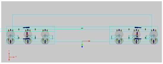
Figure 1.
Multi-body model of Co-Co locomotive in VAMPIRE environment.

Table 1.
Dynamic parameters of suspension components to be monitored.
4. Design and Configuration of Diagnostic System
4.1. Sensor Arrangements and Relevant Signal Processing Issues
The fault detection of the suspension component in the leading bogie is considered as an example of this condition monitoring scheme. The suspension monitoring system incorporates three modules: vertical, lateral and yaw modules. To guarantee the reliability of the monitoring system, only accelerometers are adopted due to their reliability in the harsh operational conditions. Figure 2 exhibits a complete sensor (accelerometer) layout for the condition monitoring of the suspension components in this locomotive bogie. In Figure 2, the red block represents the accelerometer installed on the vehicle. The arrow shows the direction of the acceleration measurement. In total, 6 accelerometers (3 triaxial and 3 biaxial), labelled as ‘W’, are mounted on the axle-boxes to measure the vertical, lateral and longitudinal accelerations of the wheelsets. Three monoaxial accelerometers, labelled as ‘M’, are installed on the motors to measure their vertical accelerations. Three accelerometers (two biaxial and one monoaxial), labelled as ‘F’, are mounted on the corners of the bogie frame to obtain the vertical, lateral and yaw accelerations of the bogie frame. One monoaxial accelerometer, labelled as ‘C’, is installed on the carbody to measure its vertical acceleration above the bogie pivot.
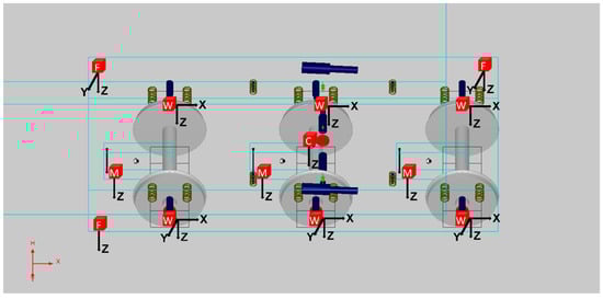
Figure 2.
Sensor layout of the proposed condition monitoring system.
Table 2 lists all the kinetic quantities needed for the parameter estimates, which are the output quantities of this locomotive model from VAMPIRE simulations. All the motions of the suspension components and the observed bogie frame accelerations can be derived readily from the acceleration signals with geometric calculations and numerical integrations [23]. It is feasible to acquire the displacement of the spring and velocity of the damper via the integrations of the relative acceleration signals. High-pass or band-pass filtering is required for the convergence of the numerical integration.
Table 2.
Kinetic quantities for RLS estimation.
In reality, not all the signal components can be used in the RLS model based on the rigid-body dynamics in the form of Equations (1) and (2). Certain high-frequency components do not follow the rigid-body dynamics and need to be eliminated by a low-pass or bandpass filtering. These components include the flexible vibration of the measured body, the local vibration from certain equipment, e.g., the motor rotor, etc. In this sense, an extensive analysis of the signal components is needed. It is necessary to mention that the sensor noise and modelling error are inevitable in the usage of this method. The error and noise can cause a certain deviation in the RLS estimate. However, if the signal is properly filtered and the model is accurate enough, the deviation in the parameter estimate can be small.
In practice, it is recommended to add more sensors to increase the redundancy of the system. Meanwhile, it is possible to reduce the less important sensors, which measure small signals or similar signals. For example, the accelerometer in carbody could be removed, since the motion of the carbody is relatively small; the sensor on the motor could be removed if the motor is connected to the bogie frame in a relatively rigid way. However, any sensor reduction should be carefully determined according to realistic vehicle behaviors. As the motion of the locomotive is very complicated, certain neglected measurements due to the sensor reductions could result in large errors in parameter estimates.
4.2. RLS Estimation Model
Correspondingly, the mathematical model for the vertical, lateral and yaw modules can be deduced according to the locomotive suspension configurations.
4.2.1. Vertical Module
The vertical module monitors the vertical suspension parameters, including primary vertical stiffness, primary vertical damping coefficients, secondary vertical stiffness, and motor link vertical stiffness and damping coefficients. In the vertical module, the regressors are the relative displacements for the primary, secondary, and motor link vertical stiffness and relative velocities for the primary vertical damping coefficients and motor link damping coefficients, 22 quantities in total. The output observation is the vertical acceleration of the bogie frame. The fundamental dynamic equation is:
where Mbf is the mass of the bogie frame.
According to the dynamic equation in the form of LS, the parameter estimate matrix is:
The regressor matrix is:
The observation is:
4.2.2. Lateral Module
The lateral module monitors the lateral parameters, including primary lateral stiffness, secondary lateral stiffness and secondary lateral damping coefficients. In the lateral module, the regressors are the relative displacements for the primary and secondary lateral stiffness, and relative velocity for the secondary lateral damper, for five quantities in total. The observation is the lateral acceleration of the bogie frame. The fundamental dynamic equation is:
The parameter estimate matrix is:
The regressor matrix is:
The observation is:
4.2.3. Yaw Module
The yaw module monitors the parameters in the yaw direction, including primary longitudinal stiffness, secondary longitudinal stiffness and secondary yaw damping. In the yaw module, the regressors are the relative displacements for primary and secondary longitudinal stiffness, relative displacements for primary and secondary lateral stiffness, and relative velocities for secondary yaw damping (eight quantities in total). The observation is the yaw acceleration of the bogie frame. The fundamental dynamic equation is:
where Jbfψ is the yaw inertia of the bogie frame. dp is the half of the lateral distance between primary longitudinal springs. lp is the half of the longitudinal distance between primary lateral springs. ds is the half of the lateral distance between secondary springs. ls is the half of the longitudinal distance between secondary springs. dd is the half of the lateral distance between the yaw dampers.
The estimate parameter matrix is:
The regressor matrix is:
The observation is:
4.2.4. Implementation of RLS in the MATLAB®/Simulink Environment
This RLS-based algorithm can be readily implemented in a MATLAB/Simulink environment with the System Identification Toolbox. Figure 3 shows a general Simulink plot for this RLS-based condition monitoring approach. The measured acceleration signals related to the suspension components are integrated into displacement or velocity signals. The measured acceleration related to the observation is multiplied with the mass or moment inertia to obtain the inertia force. The identical bandpass filtering is applied to these two sets of signals. The filtered displacement and velocity signals are fed into the ‘Regressors’ and the force signals are fed into the ‘Output’. The RLS estimator can generate convergent estimates of the suspension parameters. Due to the simplicity of this approach, the RLS-based model can be compiled with simple C/C++ codes. These complied codes can be run within a low-cost electronic device for an online monitoring application, such as Raspberry Pie.
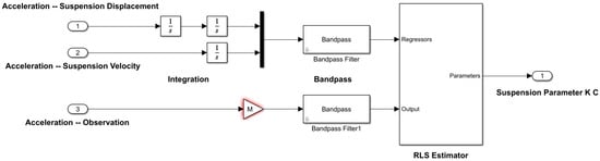
Figure 3.
Implementation of RLS approach with MATLAB/Simulink.
In addition, theoretically, it could be more efficient to use a derivative form to estimate the suspension parameters as shown in Figure 4. This means a derivative operation is applied to all the signals related to the suspensions and observations. The RLS estimator can obtain convergent results at a faster rate with this derivative form.
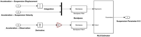
Figure 4.
Implementation of RLS approach with MATLAB/Simulink—derivative form.
5. Results of Demonstrator
To demonstrate the feasibility of the proposed condition monitoring strategy, several VAMPIRE simulations are used to generate the ‘virtual data acquisition’ for the fault-free and faulty vehicle scenarios. Both the fault-free and faulty cases utilize the same track case.
5.1. Simulation Case
The locomotive was simulated to be operating at a speed of 100 km/h on a straight track with representative track irregularities: ‘Track-160’. The conventional 56E1 rail profile (inclined at 1:20) and P8 wheel profile were utilized in the simulations. The output data generated from the simulated vehicle were exported at a sampling frequency of 1 kHz (sampling time of 1 ms), which is a common sampling frequency for acceleration measurements. A track length of 3000 m has been used in simulations. Overall, 108,000 data samples were collected for each output channel from each VAMPIRE simulation.
The VAMPIRE output data were converted into the required variables in the MATLAB workspace. Simulink reads these variables into the RLS block as regressors and an observation. The data exported from the RLS block are the time series of the estimated suspension parameters. To obtain the most robust estimate of the parameter from the RLS estimator, the forgetting factor of RLS is set as 1.
5.2. Suspension Fault Case
To investigate the feasibility of this parameter-based fault detection approach, several ‘artificial’ suspension faults were incorporated into the leading bogie of the VAMPIRE vehicle model. These suspension faults included:
- Damping coefficients of secondary yaw dampers, which are set to zero;
- Damping coefficients of secondary lateral dampers, which are set to zero;
- The stiffness of one secondary vertical rubber spring (front right), set to 2 times its normal stiffness value;
- Primary lateral stiffness and longitudinal stiffness of one primary rubber bushing (leading right), set to be 2 times their normal values.
A higher stiffness is likely to be indicative of a degraded rubber spring component due to the loss of flexibility. These suspension faults are only general examples of possible fault scenarios selected to demonstrate the concept explored in this study. In Figure 5, the suspension components with faults are marked with circles. Note that the fault case used here is only for the demonstration of the potential of the diagnostic system. In reality, a single component failure is the most common fault, such as a yaw damper failure.
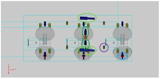
Figure 5.
Bogie plot with marked faulty suspension elements.
5.3. Comparisons of RLS Estimation Results
Corresponding to the track case above, transient simulations were carried out in VAMPIRE regarding the fault-free vehicle model and the faulty vehicle model. The vibration signals exported from the VAMPIRE simulations were introduced into the three modules of the Simulink models for parameter estimations. All the output channels are related to the front bogie. From the simulation results, it is very difficult to distinguish the abnormal behaviors of the faulty vehicle from the resulting vibration signals compared with a fault-free vehicle. Using the previously mentioned Simulink models in derivative forms, several key parameters were estimated for both vehicle models, and the comparisons are shown below.
In the following figures, the arrow represents the parameter values used in the simulations. The color of the arrow corresponds to that of the estimation curve, referring to the same quantity. The black arrow pinpoints the nominal value used in the simulations.
5.3.1. Lateral Module Results
From the lateral module, the secondary lateral damping coefficient and primary lateral stiffness can be estimated.
The estimated secondary lateral damping coefficient of the fault-free vehicle is shown in Figure 6a. It has a nominal value of 75 kNs/m (per damper) in the simulated model, shown as the blue arrow in Figure 6a. The estimated secondary lateral damping coefficient of the faulty vehicle is shown in Figure 6b. Its value set in the simulation model is zero, shown as the blue arrow in Figure 6b. Figure 6b shows that the RLS correctly estimates a very small value for the damping coefficient, indicating a degraded condition.
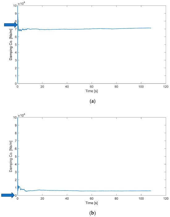
Figure 6.
Estimate of secondary lateral damping coefficient. (a) Fault-free case; (b) faulty case.
For the fault-free vehicle, the estimated primary lateral stiffness of three axles is shown in Figure 7a. In this nominal condition, the front and rear axles have a large lateral stiffness of 10.5 MN/m per bushing (shown as the black arrow in Figure 7a), while the middle axle has a very small stiffness of 0.5 MN/m per bushing (shown as the yellow arrow in Figure 7a). The estimate of the primary lateral stiffness of the faulty vehicle is shown in Figure 7b. Here, in this faulty vehicle model, the lateral stiffness of the front axle should be 15.5 MN/m (the average of two bushings, shown as the blue arrow in Figure 7b). The estimate of the primary lateral stiffness of the front axle is very similar to this value. Meanwhile, the stiffness estimates for the rear and middle axles are still approximate to their nominal values (shown as the red and yellow arrows, respectively, in Figure 7b).
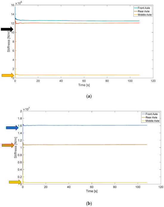
Figure 7.
Estimate of primary lateral stiffness. (a) Fault-free case; (b) faulty case.
The estimates of the secondary lateral damping coefficient and primary lateral stiffness are very closely matched to the values defined in the VAMPIRE models. Therefore, the fault diagnoses of the secondary lateral damper and primary lateral springs could be achieved using this lateral module.
5.3.2. Yaw Module Results
From the yaw module, the damping coefficient of the secondary yaw damper, primary longitudinal stiffness, and primary lateral stiffness (front and rear axles) can be estimated.
The estimated damping coefficient of the secondary yaw damper of the fault-free vehicle is shown in Figure 8a. Its nominal value in this simulation model is 150 kNs/m per damper, shown as the blue arrow in Figure 8a. For the faulty case, the estimated damping coefficient of the secondary yaw damper is shown in Figure 8b. Its value in this simulation is zero, shown as the blue arrow in Figure 8b. Figure 8b shows that the yaw module estimates a very small value for the damping coefficient, indicating a degraded condition.
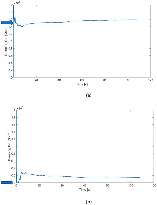
Figure 8.
Estimate of secondary yaw damping coefficient. (a) Fault-free case; (b) faulty case.
For the fault-free vehicle, the primary longitudinal stiffness of three axles is shown in Figure 9a. Its nominal value for each axle is 30 MN/m per bushing, shown as the black arrow in Figure 9a. For the faulty vehicle, the estimate of primary longitudinal stiffness is shown in Figure 9b. In this case, the longitudinal stiffness value of the front axle should be 45 MN/m (per bushing, average of a pair of bushings), shown as the blue arrow in Figure 9b. From Figure 9b, the estimates for the rear and middle axles are almost identical to the nominal values (shown as the black arrow in Figure 9b). The estimate for the front axle is higher than the others and similar to the value used in the simulation.
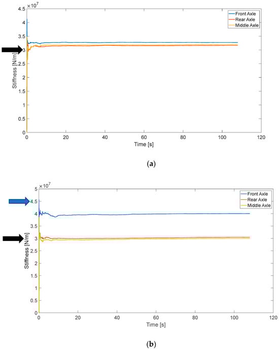
Figure 9.
Estimate of primary longitudinal stiffness. (a) Fault-free case; (b) faulty case.
The estimates of the damping coefficient of the yaw damper and primary longitudinal stiffness correlate well with the values defined in the VAMPIRE simulation models. In fact, the primary lateral stiffness of leading and trailing axles can be estimated in yaw module with consistent results as well. Therefore, the fault detections and isolations of these suspension components in the yaw direction could be achieved by this module.
5.3.3. Vertical Module Results
From the vertical module, the estimate of the secondary vertical stiffness of the fault-free vehicle is shown in Figure 10a, which has a nominal value of 10 MN/m (per spring) in the simulation model (shown as the black arrow in Figure 10a). It is clear that all the stiffness estimates are very accurate. The estimate of the secondary vertical stiffness of the faulty vehicle is shown in Figure 10b. In this simulation model, the stiffness value of the front right rubber spring is set to be 20 MN/m, shown as the blue arrow in Figure 10b. The other springs still have nominal values of 10 MN/m, shown as the black arrow in Figure 10b. From Figure 10b, the stiffness estimate of the front right spring is definitely higher than the other estimates. Although this vertical model does not deliver very accurate estimates due to the similarities of signals, it is obvious that some variation from the nominal value can be detected for the secondary springs. Figure 11 shows the estimate of the motor link stiffness of the fault-free vehicle, which has a nominal value in the simulation model of 10 MN/m per link (shown as the black arrow in Figure 11). These three estimates are approximate to the simulation value.
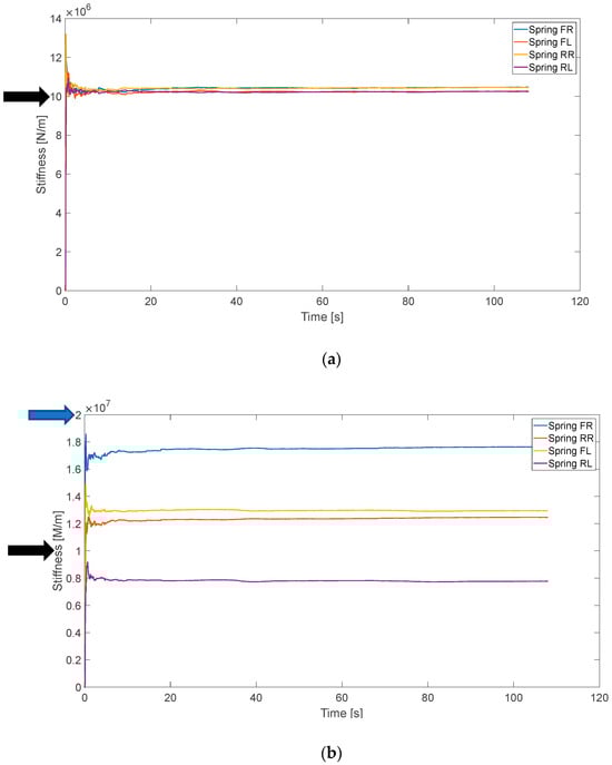
Figure 10.
Estimate of secondary vertical stiffness. (a) Fault-free case; (b) faulty case.
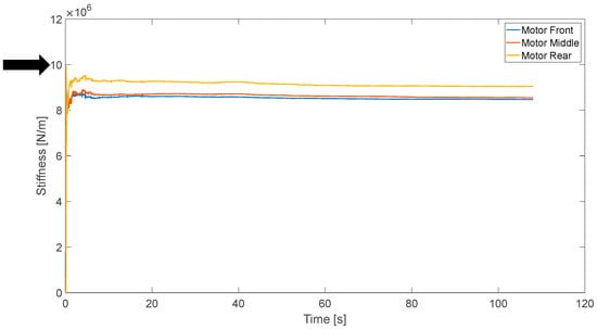
Figure 11.
Estimate of motor link stiffness—fault-free case.
Due to the suspension configuration of this vehicle, the damping coefficient of the primary vertical damper and the stiffness of the primary vertical spring are relatively small. In this sense, the vertical acceleration of the bogie frame mainly reflects the suspension forces generated by the secondary vertical spring and the motor link, which are of large stiffness. The weak forces generated by the primary suspension components are difficult to be estimated accurately from the vertical acceleration of the bogie frame. Similarly, the horizontal stiffness of the secondary spring is also difficult to estimate accurately from the lateral or yaw modules due to its small value, since it is not easy to observe its small spring force/torque from the lateral/yaw acceleration of the bogie frame. Moreover, the parameter estimates of these ‘soft’ suspension components are still in the same scales with the values in the simulation models.
6. Conclusions and Discussion
This study aimed to provide a universal platform for the development of a condition monitoring system for rail vehicle suspension components. A condition monitoring scheme is demonstrated with the fault diagnosis of a Co-Co locomotive suspension system. It is obvious that the suspension is a coupled dynamics system since each suspension component affects vehicle dynamic behavior simultaneously. Therefore, the decoupling of the contributions from suspension components becomes an essential issue. In this background, the model-based method, which is capable of estimating the suspension parameters directly from a dynamic system, paves a potential way to solve this problem.
Oriented towards the fault diagnosis of the suspension system with a decoupling approach, an efficient RLS-based condition monitoring solution for the locomotive suspension is shown in this demonstrator. RLS has machine learning features and can identify multiple parameters simultaneously from a parametric model. The parametric model can be determined readily because the acceleration of the sprung mass equals the sum of the corresponding suspension loads. This constitutes a least-square problem for parameter estimation with an over-determined algebraic equation set. In this sense, with the optimal Kalman gain, the RLS is highly suitable for the parameter identification from such a coupled system to realize the diagnosis of the suspension component.
Correspondingly, a condition monitoring scheme for the vehicle suspension was designed and configured with a Co-Co locomotive concerned. In this condition monitoring system, three modules were developed in accordance with the suspension layout of this locomotive. The three modules include a vertical module, a lateral module and a yaw module, which are formulated in a MATLAB/Simulink environment. The simulation results from the multi-body software VAMPIRE are employed as a ‘virtual data acquisition’ system to demonstrate the proposed approach. In the multi-body simulations, several faults are considered simultaneously in the suspension system, including the damper failures and spring degradations. From the results of the demonstrator, the suspension parameter estimates are consistent with the values used in the multi-body simulations, providing a straightforward result for the fault detection and isolation. These results provide supporting evidence to demonstrate the application of the proposed condition monitoring scheme for the detection of faults in the suspension system of a rail vehicle.
Additionally, due to the simplicity of this CBM algorithm, an online suspension monitoring system could be feasible with a low-cost electronic computing device, such as a Raspberry Pi. There is the potential for more advanced in-service deployment and condition-based maintenance to be developed. The diagnostic information of the suspension system can be transmitted to the driver’s cabin via the vehicle bus. The driver can make a decision according to diagnostic information. For example, the driver can decide to reduce the vehicle speed to a safety level if a severe suspension fault is detected. Meanwhile, the diagnostic information can be transmitted to the depot by the vehicle antenna via a suitable communication protocol. When the train with the diagnosed suspension fault returns to the depot, the replacement or repairment of the faulty suspension component be carried out promptly.
Author Contributions
Conceptualization, X.L. and A.B.; methodology, X.L.; software, X.L.; validation, X.L.; formal analysis, X.L.; investigation, X.L.; resources, X.L. and A.B.; data curation, X.L.; writing—original draft preparation, X.L.; writing—review and editing, A.B. and X.L.; visualization, X.L.; supervision, A.B.; project administration, A.B.; funding acquisition, A.B. All authors have read and agreed to the published version of the manuscript.
Funding
This research was funded by EU Horizon2020 Shift2Rail LOCATE (Locomotive bOgie Condition mAinTEnance) project, grant number 881805.
Data Availability Statement
The original contributions presented in this study are included in the article. Further inquiries can be directed to the corresponding author.
Conflicts of Interest
The authors declare no conflicts of interest. The funders had no role in the design of the study; in the collection, analyses, or interpretation of data; in the writing of the manuscript; or in the decision to publish the results.
Abbreviations
The following abbreviations are used in this manuscript:
| RLS | Recursive least-square |
| CBM | Condition-based monitoring |
| KF | Kalman filter |
References
- Bruni, S.; Goodall, R.; Mei, T.X.; Tsunashima, H. Control and monitoring for railway vehicle dynamics. Veh. Syst. Dyn. 2007, 45, 743–799. [Google Scholar] [CrossRef]
- Ward, C.P.; Weston, P.F.; Stewart, E.J.C.; Li, H.; Goodall, R.M.; Roberts, C.; Mei, T.X.; Charles, G.; Dixon, R. Condition monitoring opportunities using vehicle-based sensors. Part F J. Rail Rapid Transit 2011, 225, 202–218. [Google Scholar] [CrossRef]
- Gasparetto, L.; Alfi, S.; Bruni, S. Data-driven condition-based monitoring of high-speed railway bogies. Int. J. Rail Transp. 2013, 1, 42–56. [Google Scholar] [CrossRef]
- Mei, T.X.; Ding, X.J. Condition monitoring of rail vehicle suspensions based on changes in system dynamic interactions. Vehicle Syst. Dyn. 2009, 49, 1167–1181. [Google Scholar] [CrossRef]
- Melnik, R.; Seweryn, K. Rail Vehicle Suspension Condition Monitoring—Approach and Implementation. J. Vibroengineering 2017, 19, 487–501. [Google Scholar] [CrossRef]
- Dumitriu, M. Condition Monitoring of the Dampers in the Railway Vehicle Suspension Based on the Vibrations Response Analysis of the Bogie. Sensors 2022, 22, 3290. [Google Scholar] [CrossRef] [PubMed]
- Hong, N.; Li, L.; Yao, W.; Zhao, Y.; Yi, C.; Lin, J.; Tsui, K.L. High-Speed Rail Suspension System Health Monitoring Using Multi-Location Vibration Data. IEEE Trans. Intell. Transp. Syst. 2020, 21, 2943–2955. [Google Scholar] [CrossRef]
- Lebel, D.; Soize, C.; Funfschilling, C.; Perrin, G. High-speed train suspension health monitoring using computational dynamics and acceleration measurements. Vehicle Syst. Dyn. 2019, 58, 911–932. [Google Scholar] [CrossRef]
- Liu, F.; Gu, F.; Ball, A.D.; Zhao, Y.; Peng, B. The validation of an ACS-SSI based online condition monitoring for railway vehicle suspension systems using a SIMPACK model. In Proceedings of the IEEE 23rd International Conference on Automation and Computing (ICAC), Huddersfield, UK, 7–8 September 2017. [Google Scholar]
- Karlsson, H.; Qazizadeh, A.; Stichel, S.; Berg, M. Condition Monitoring of Rail Vehicle Suspension Elements: A Machine Learning Approach. In Proceedings of the 26th Symposium of the International Association of Vehicle System Dynamics, IAVSD 2019, Gothenburg, Sweden, 12–16 August 2019. [Google Scholar]
- Chen, Y.; Niu, G.; Li, Y.; Li, Y. A modified bidirectional long short-term memory neural network for rail vehicle suspension fault detection. Vehicle Syst. Dyn. 2022, 61, 3136–3160. [Google Scholar] [CrossRef]
- Li, P.; Goodall, R.; Weston, P.; Ling, C.S.; Goodman, C.; Roberts, C. Estimation of railway vehicle suspension parameters for condition monitoring. Control Eng. Pract. 2007, 15, 43–55. [Google Scholar] [CrossRef]
- Tsunashima, H.; Mori, H. Condition monitoring of railway vehicle suspension using adaptive multiple model approach. In Proceedings of the International Conference on Control, Automation and Systems, Kintex, Gyeonggi-do, Republic of Korea, 27–30 October 2010. [Google Scholar]
- Jesussek, M.; Ellermann, K. Fault detection and isolation for a nonlinear railway vehicle suspension with a Hybrid Extended Kalman filter. Vehicle Syst. Dyn. 2013, 51, 1489–1501. [Google Scholar] [CrossRef]
- Zoljic-Beglerovic, S.; Stettinger, G.; Luber, B.; Horn, M. Railway Suspension System Fault Diagnosis using Cubature Kalman Filter Techniques. IFAC-Pap. 2018, 51, 1330–1335. [Google Scholar] [CrossRef]
- Isermann, R.; Muenchhof, M. Identification of Dynamic Systems; Springer: Berlin/Heidelberg, Germany, 2011. [Google Scholar]
- Jakubek, S.; Kozek, M. Control and identification. In Road and off-Road Vehicle System Dynamics Handbook; Mastinu, G.R., Ploechl, M., Eds.; CRC Press, Taylor & Francis: Boca Raton, FL, USA, 2014; pp. 159–219. [Google Scholar]
- Young, P.C. Recursive Estimation and Time-Series Analysis, 2nd ed.; Springer: Berlin/Heidelberg, Germany, 2011. [Google Scholar]
- Diniz, P.S. Adaptive Filtering: Algorithms and Practical Implementation, 4th ed.; Springer: New York, NY, USA, 2013. [Google Scholar]
- Uncini, A. Fundamentals of Adaptive Signal Processing; Springer: Cham, Switzerland, 2015. [Google Scholar]
- Keesman, K.J. System Identification; Springer: London, UK, 2011. [Google Scholar]
- Vega, L.R.; Rey, H. A Rapid Introduction to Adaptive Filtering; Springer: Berlin/Heidelberg, Germany, 2013. [Google Scholar]
- Liu, X. An Efficient Condition Monitoring Approach for Railway Vehicle Suspension System by Using Model-Based Assessment. Ph.D. Thesis, Politecnico di Milano, Milan, Italy, 2016. [Google Scholar]


Disclaimer/Publisher’s Note: The statements, opinions and data contained in all publications are solely those of the individual author(s) and contributor(s) and not of MDPI and/or the editor(s). MDPI and/or the editor(s) disclaim responsibility for any injury to people or property resulting from any ideas, methods, instructions or products referred to in the content. |
© 2025 by the authors. Licensee MDPI, Basel, Switzerland. This article is an open access article distributed under the terms and conditions of the Creative Commons Attribution (CC BY) license (https://creativecommons.org/licenses/by/4.0/).