Fractional-Order LC Three-Phase Inverter Using Fractional-Order Virtual Synchronous Generator Control and Adaptive Rotational Inertia Optimization

Abstract

The application of fractional calculus in power electronics modeling provides an innovative method for improving inverter performance. This paper presents a three-phase inverter topology with fractional-order LC filter characteristics, analyzes its frequency response, and develops mathematical models in both stationary and rotating reference frames. Based on these models, a dual closed-loop decoupling control strategy for voltage and current is designed to enhance system stability and dynamic performance. In the power control loop, fractional-order virtual synchronous generator control (FOVSG) is employed. Observations show that increasing the fractional-order of the rotor leads to a higher transient frequency variation rate. To address this, an adaptive rotational inertia control scheme is integrated into the FOVSG structure (ADJ-FOVSG), enabling real-time adjustment of inertia to suppress transient frequency fluctuations. Experimental results demonstrate that when the reference active power changes, ADJ-FOVSG effectively suppresses power overshoot. Compared to traditional VSG, ADJ-FOVSG reduces the power regulation time by approximately 34.5% and decreases the peak frequency deviation by approximately 37.2%. Compared to the adaptive rotational inertia control in traditional VSG, ADJ-FOVSG improves regulation time by about 24% and reduces peak frequency deviation by roughly 24.4%.

1. Introduction

Currently, most control systems defined by differential equations use integer-order derivatives. Many real-world systems exhibit fractional-order characteristics. Using fractional-order derivatives enables a more accurate capture of their dynamic behavior. As science and technology advance and our understanding of natural systems deepens, fractional calculus has found broad applicability across various domains [1]. In electrical engineering, growing evidence suggests that inductors and capacitors inherently exhibit fractional-order behavior, and fractional calculus offers a more accurate modeling framework. Concurrently, scholars are developing new methods for analyzing and designing fractional-order inductors and capacitors [2,3,4,5,6,7,8,9]. The fractional-order characteristics of inductors and capacitors have had a significant impact on power electronic converter research, influencing topology design, modeling, analysis, and control strategies, and opening up a new research direction.

Integrating fractional-order inductors and fractional-order capacitors into power electronics topologies allows for a more accurate representation of their inherent dynamic behavior. Research on fractional-order power electronic converters has mainly focused on DC/DC converters [10,11,12,13]. Recently, the research scope has expanded to include fractional-order rectifiers [14,15], inverters [16,17,18,19,20,21,22], and static compensators [23,24]. Findings suggest that fractional-order models more accurately represent the actual operating conditions of power electronic equipment. Fractional calculus is widely used in controller design, where adjustable fractional-order parameters improve control performance. Fractional-order controllers commonly used in power systems include fractional-order PID control [14,17,19], fractional-order sliding mode control [23], and fractional-order active disturbance rejection control [25], highlighting their potential to enhance control performance.

In modern power systems, distributed generation control frameworks primarily connect renewable energy to the grid through grid-connected inverters. This approach offers significant advantages in control flexibility and response speed over conventional synchronous generator connections. However, the inherent randomness and volatility of large-scale distributed power source integration can significantly affect grid stability, imposing stricter performance requirements on three-phase inverters as critical components [26,27]. Research on traditional three-phase inverters is well established, with fractional calculus recognized as a novel method for improving inverter performance. Current research primarily focuses on integrating fractional-order inductors and fractional-order capacitors into inverter topologies and applying fractional-order controllers, such as fractional-order models and fractional-order control.

In the context of fractional-order modeling, Ref. [16] developed a fractional-order model of a single-phase inverter over one switching cycle. The study employed the state-space averaging method to derive a small-signal model, showing that it more closely approximates the real system. Ref. [17] proposed high- and low-frequency models for a fractional-order three-phase L-type grid-connected inverter and designed a decoupled control structure for the fractional-order current inner loop. Simulation results indicate that the system achieves improved dynamic and static performance, significantly enhancing grid power quality compared to traditional integer-order systems. Ref. [19] integrated a fractional-order LCL filter into a grid-side inverter for wind power generation and applied fractional-order PI controllers for its control. By properly selecting the fractional orders of the filter’s capacitor and inductor, the resonance issue inherent in traditional LCL filters was effectively mitigated. Simulations demonstrated that a fully fractional-order grid-side inverter system significantly improves grid power factor and DC-link voltage regulation compared to an integer-order system. These studies suggest that fractional-order models more accurately represent real systems and better capture the true operational behavior of converters.

In the context of fractional-order control, extensive research has been conducted on applying fractional-order PI control to three-phase inverters. However, with increasing renewable energy penetration, the low inertia and undamped characteristics of power electronic devices have negatively impacted power system stability. Virtual synchronous generator (VSG) control, which emulates the frequency and voltage behavior of synchronous generators, has emerged as a promising solution [28]. This control strategy allows three-phase inverters to replicate synchronous generator characteristics, supplying inertia and damping to mitigate voltage and frequency fluctuations on the grid [29]. Given these advantages, exploring fractional-order characteristics within VSG control has become particularly relevant. Ref. [20] introduces a virtual synchronous generator incorporating fractional-order virtual inertia. Compared to conventional VSG technology using first-order inertia, this method effectively suppresses active power oscillations and improves the performance of grid-connected inverters. Ref. [21] proposes an optimized active response strategy for VSG, incorporating fractional-order derivative correction. This strategy introduces a fractional-order correction component into conventional VSG active control, effectively reducing dynamic oscillations and overshoots in active power. Ref. [22] presents a novel fractional-order virtual synchronous generator (FOVSG) control scheme and provides a detailed controller design. Experimental results confirm the superior performance of FOVSG control in both grid-connected and islanded modes. These studies demonstrate that integrating fractional-order control into controller design enhances flexibility and leads to improved performance.

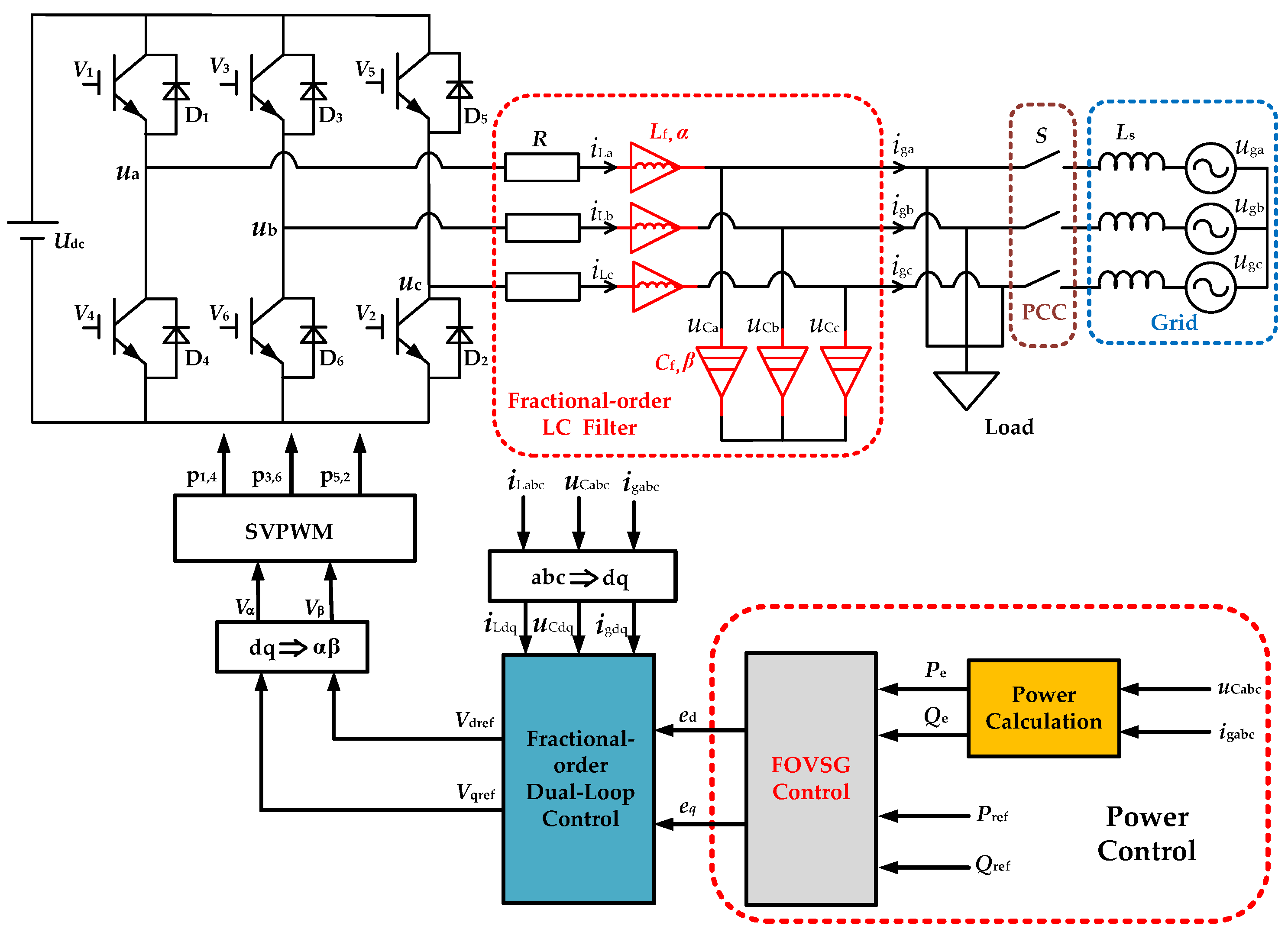
Current research on VSG control predominantly employs integer-order models, frequently overlooking the intrinsic fractional-order characteristics of inductors and capacitors. This paper proposes a fractional-order LC three-phase inverter using fractional-order virtual synchronous generator control and adaptive rotational inertia optimization. The main contributions of this study are summarized as follows:

• A mathematical model of the fractional-order three-phase LC inverter is established in both the three-phase stationary coordinate system and the synchronously rotating coordinate system.
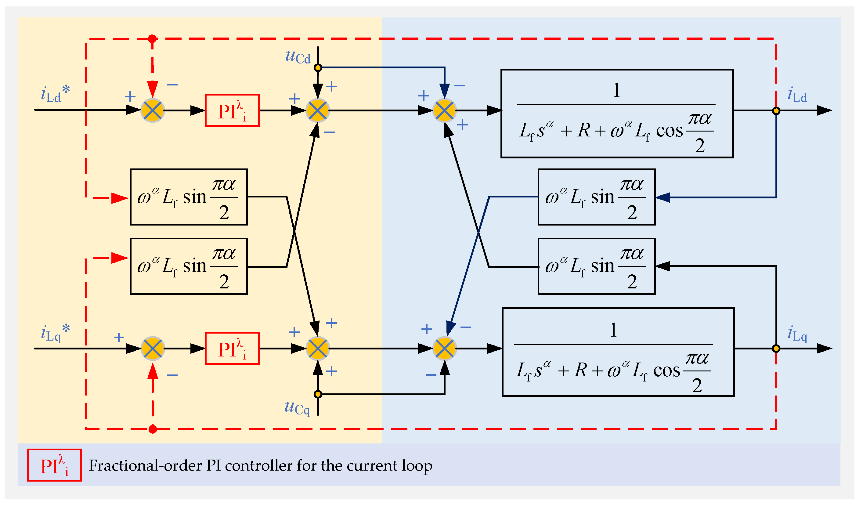
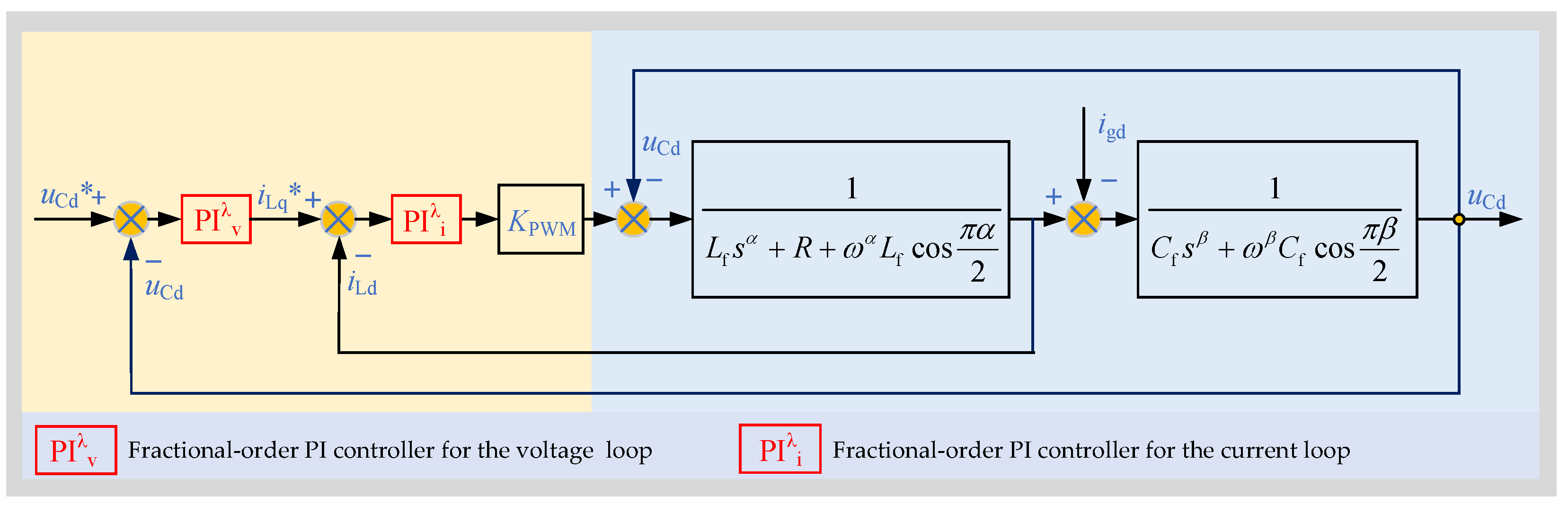
• A fractional-order decoupling control structure with voltage and current loops is designed to implement d–q axis decoupling control for the fractional-order three-phase LC inverter.
• An FOVSG with adaptive rotational inertia optimization is developed to improve the inverter’s dynamic response under disturbances.

The paper is structured as follows: Section 2 introduces the fractional-order three-phase inverter system and the implementation of fractional calculus operators. Section 3 elaborates on the fractional-order model of the three-phase inverter, encompassing the mathematical model, characteristics of the fractional-order LC filter, and the dual closed-loop control strategy. Section 4 analyzes the FOVSG control strategy, covering its principles, stability assessment, and adaptive rotational inertia control. Section 5 presents digital simulation analysis. Section 6 provides the discussion. Section 7 concludes with a summary of key findings.

2. System Description of the Fractional-Order Three-Phase Inverter

2.1. System Description

Fractional-order inductors and capacitors are essential components of fractional-order circuits. The circuit symbols used in this paper are shown in Figure 1.

Here, L and C represent the inductance and capacitance of fractional-order inductors and fractional-order capacitors, while $\alpha$ and $\beta$ denote their corresponding fractional orders. The voltage and current of the fractional-order inductor are denoted as $u_{\mathrm{L}}$ and $i_{\mathrm{L}}$, and the voltage and current of the fractional-order capacitor are denoted as $u_{\mathrm{C}}$ and $i_{\mathrm{C}}$.

The mathematical models for the fractional-order inductor and fractional-order capacitor are presented in Equation (1), forming the foundation for fractional-order circuit analysis.

$$\left\{\begin{array}{c}{u}_{\mathrm{L}}=L{\displaystyle \frac{{\mathrm{d}}^{\alpha }{i}_{\mathrm{L}}}{\mathrm{d}{t}^{\alpha }}},\alpha \in (0,2)\hfill \\ i_{\mathrm{C}}=C{\displaystyle \frac{{\mathrm{d}}^{\beta }{u}_{\mathrm{C}}}{\mathrm{d}{t}^{\beta }}},\beta \in (0,2)\hfill \end{array}\right.$$

(1)

Figure 2 shows the structure of the fractional-order three-phase inverter system used in this study. The DC side of the inverter is composed of an ideal DC source. The primary circuit incorporates the fractional-order characteristics of the LC filter, resulting in a fractional-order three-phase LC inverter topology. The control section mainly consists of FOVSG control and fractional-order dual-loop control. Here, $U_{\mathrm{dc}}$ represents the DC-side voltage, and $L_{\mathrm{f}}$ and $C_{\mathrm{f}}$ denote the inductance and capacitance of the fractional-order filter, with $\alpha$ and $\beta$ indicating their respective fractional orders. R is the damping resistor, $L_{\mathrm{s}}$ is the line inductance, ${\mathit{u}}_{\mathrm{abc}}$ represents the inverter output voltage, and ${\mathit{i}}_{\mathrm{Labc}}$ and ${\mathit{u}}_{\mathrm{Cabc}}$ denote the current through the fractional-order inductor and the voltage across the fractional-order capacitor, respectively. ${\mathit{i}}_{\mathrm{gabc}}$ represents the line current, $Q_{\mathrm{e}}$ and $Q_{\mathrm{ref}}$ denote the measured and reference reactive powers, $P_{\mathrm{e}}$ and $P_{\mathrm{ref}}$ indicate the measured and reference active powers, ${\mathit{i}}_{\mathrm{Ldq}}$, ${\mathit{u}}_{\mathrm{Cdq}}$, and ${\mathit{i}}_{\mathrm{gdq}}$ represent the dq-transformed values of ${\mathit{i}}_{\mathrm{Labc}}$, ${\mathit{u}}_{\mathrm{Cabc}}$, and ${\mathit{i}}_{\mathrm{gabc}}$, respectively. $e_{\mathrm{d}}$ and $e_{\mathrm{q}}$ are the dq-transformed synthesized three-phase electromotive forces of the FOVSG, and $V_{\mathrm{dref}}$ and $V_{\mathrm{qref}}$ represent the d-axis and q-axis reference values output by the fractional-order dual-loop control.

2.2. Implementation of Fractional Calculus Operators

In this paper, the fractional-order operator $s^{\gamma }$ is approximated by the Oustaloup’s recursive filter [30]. Using the Oustaloup approximation algorithm, simulation models for fractional-order inductors and fractional-order capacitors are constructed. The standard form of the Oustaloup filter is as follows:

$$s^{\gamma }=K\prod _{k=1}^N{\displaystyle \frac{s+{\omega }_k^{\prime }}{s+{\omega }_k}}$$

(2)

where $\gamma$ is the order of the fractional part, and N represents the filter order. The expressions for K, ${\omega }_k^{\prime }$, and ${\omega }_k$ are as follows:

$$\left\{\begin{array}{c}K={\omega }_{\mathrm{h}}^{\gamma },{\omega }_{\mathrm{u}}=\sqrt{{\omega }_{\mathrm{h}}/{\omega }_{\mathrm{l}}}\hfill \\ {\omega }_{\mathrm{k}}^{\prime }={\omega }_{\mathrm{l}}{\omega }_{\mathrm{u}}^{(2k-1-\gamma )/N},{\omega }_{\mathrm{k}}={\omega }_{\mathrm{l}}{\omega }_{\mathrm{u}}^{(2k-1+\gamma )/N}\hfill \end{array}\right.$$

(3)

where ${\omega }_{\mathrm{l}}$ and ${\omega }_{\mathrm{h}}$ denote the lower and upper bounds of the selected frequency, respectively. Considering design precision and complexity, this paper sets the filter order N to 7, with ${\omega }_{\mathrm{l}}$ and ${\omega }_{\mathrm{h}}$ as ${10}^{-2}$ rad/s and ${10}^6$ rad/s, respectively.

3. Fractional-Order Three-Phase Inverter

3.1. Mathematical Modeling of Fractional-Order Three-Phase Inverters

For the inverter topology in Figure 2, under three-phase symmetry, applying Kirchhoff’s voltage and current laws while accounting for the fractional-order characteristics of the filter capacitors and inductors yields the following mathematical model in the three-phase stationary coordinate system:

$$\left\{\begin{array}{c}{L}_{\mathrm{f}}{\displaystyle \frac{{\mathrm{d}}^{\alpha }{\mathit{i}}_{\mathrm{Labc}}}{\mathrm{d}{t}^{\alpha }}}={\mathit{u}}_{\mathrm{abc}}-R{\mathit{i}}_{\mathrm{Labc}}-{\mathit{u}}_{\mathrm{Cabc}}\hfill \\ C_{\mathrm{f}}{\displaystyle \frac{{\mathrm{d}}^{\beta }{\mathit{u}}_{\mathrm{Cabc}}}{\mathrm{d}{t}^{\beta }}}={\mathit{i}}_{\mathrm{Labc}}-{\mathit{i}}_{\mathrm{gabc}}\hfill \end{array}\right.$$

(4)

To facilitate controller design, it is necessary to transform the mathematical model from the three-phase stationary reference frame to the synchronously rotating reference frame. The transformation matrix is given by

$$\mathit{P}={\mathit{T}}_{\mathrm{abc}/\mathrm{dq}0}={\displaystyle \frac{2}{3}}\left[\begin{array}{ccc}cos\left(\omega t\right)& cos(\omega t-{\displaystyle \frac{2\pi }{3}})& cos(\omega t+{\displaystyle \frac{2\pi }{3}})\\ -sin\left(\omega t\right)& -sin(\omega t-{\displaystyle \frac{2\pi }{3}})& -sin(\omega t+{\displaystyle \frac{2\pi }{3}})\\ {\displaystyle \frac{1}{2}}& {\displaystyle \frac{1}{2}}& {\displaystyle \frac{1}{2}}\end{array}\right]$$

(5)

where $\omega$ denotes the synchronous rotational angular velocity.

The inverse transformation matrix of Equation (5) is as follows:

$${\mathit{P}}^{-1}={\mathit{T}}_{\mathrm{dq}0/\mathrm{abc}}^{-1}=\left[\begin{array}{ccc}cos\left(\omega t\right)& -sin\left(\omega t\right)& 1\\ cos\left(\omega t-{\displaystyle \frac{2\pi }{3}}\right)& -sin\left(\omega t-{\displaystyle \frac{2\pi }{3}}\right)& 1\\ cos\left(\omega t+{\displaystyle \frac{2\pi }{3}}\right)& -sin\left(\omega t+{\displaystyle \frac{2\pi }{3}}\right)& 1\end{array}\right]$$

(6)

By combining Equations (4) and (5), the result is obtained:

$$\left\{\begin{array}{c}{L}_{\mathrm{f}}\mathit{P}{\displaystyle \frac{{\mathrm{d}}^{\alpha }{\mathit{i}}_{\mathrm{Labc}}}{{\mathrm{d}}^{\alpha }t}}=\mathit{P}{\mathit{u}}_{\mathrm{abc}}-R\mathit{P}{\mathit{i}}_{\mathrm{Labc}}-\mathit{P}{\mathit{u}}_{\mathrm{Cabc}}\hfill \\ C_{\mathrm{f}}\mathit{P}{\displaystyle \frac{{\mathrm{d}}^{\beta }{\mathit{u}}_{\mathrm{Cabc}}}{{\mathrm{d}}^{\beta }t}}=\mathit{P}{\mathit{i}}_{\mathrm{Labc}}-\mathit{P}{\mathit{i}}_{\mathrm{gabc}}\hfill \end{array}\right.$$

(7)

According to the differentiation rule, for the three-phase variable ${\mathit{x}}_{\mathrm{abc}}$, it can be expressed as follows:

$$\mathit{P}{\displaystyle \frac{{\mathrm{d}}^{\alpha }{\mathit{x}}_{\mathrm{abc}}}{{\mathrm{d}}^{\alpha }t}}={\displaystyle \frac{{\mathrm{d}}^{\alpha }\left(\mathit{P}{\mathit{x}}_{\mathrm{abc}}\right)}{{\mathrm{d}}^{\alpha }t}}-{\displaystyle \frac{{\mathrm{d}}^{\alpha }\mathit{P}}{{\mathrm{d}}^{\alpha }t}}{\mathit{x}}_{\mathrm{abc}}={\displaystyle \frac{{\mathrm{d}}^{\alpha }{\mathit{x}}_{\mathrm{dq}0}}{{\mathrm{d}}^{\alpha }t}}-{\displaystyle \frac{{\mathrm{d}}^{\alpha }\mathit{P}}{{\mathrm{d}}^{\alpha }t}}{\mathit{P}}^{-1}{\mathit{x}}_{\mathrm{dq}0}$$

(8)

The fractional-order derivative form of the transformation matrix shown in Equation (5) can be expressed as

$${\displaystyle \frac{{\mathrm{d}}^{\alpha }\mathit{P}}{\mathrm{d}{t}^{\alpha }}}={\displaystyle \frac{2}{3}}\left[\begin{array}{ccc}x& -{\displaystyle \frac{1}{2}}x+{\displaystyle \frac{\sqrt{3}}{2}}y& -{\displaystyle \frac{1}{2}}x-{\displaystyle \frac{\sqrt{3}}{2}}y\\ -y& {\displaystyle \frac{1}{2}}y+{\displaystyle \frac{\sqrt{3}}{2}}x& {\displaystyle \frac{1}{2}}y-{\displaystyle \frac{\sqrt{3}}{2}}x\\ 0& 0& 0\end{array}\right]$$

(9)

where $x={\omega }^{\alpha }cos\left(\omega t+{\displaystyle \frac{\alpha \pi }{2}}\right)$ and $y={\omega }^{\alpha }sin\left(\omega t+{\displaystyle \frac{\alpha \pi }{2}}\right)$.

By applying the transformation defined in Equation (8) to the three-phase vectors in Equation (7), the mathematical model of the fractional-order LC three-phase inverter in the synchronous rotating reference frame is derived as follows:

$$\left\{\begin{array}{c}{L}_{\mathrm{f}}{\displaystyle \frac{{\mathrm{d}}^{\alpha }{i}_{\mathrm{Ld}}}{\mathrm{d}{t}^{\alpha }}}=u_{\mathrm{d}}-u_{\mathrm{Cd}}-\left(R+L_{\mathrm{f}}{\omega }^{\alpha }cos{\displaystyle \frac{\pi \alpha }{2}}\right)i_{\mathrm{Ld}}+L_{\mathrm{f}}{\omega }^{\alpha }sin{\displaystyle \frac{\pi \alpha }{2}}{i}_{\mathrm{Lq}}\hfill \\ L_{\mathrm{f}}{\displaystyle \frac{{\mathrm{d}}^{\alpha }{i}_{\mathrm{Lq}}}{\mathrm{d}{t}^{\alpha }}}=u_{\mathrm{q}}-u_{\mathrm{Cq}}-\left(R+L_{\mathrm{f}}{\omega }^{\alpha }cos{\displaystyle \frac{\pi \alpha }{2}}\right)i_{\mathrm{Lq}}-L_{\mathrm{f}}{\omega }^{\alpha }sin{\displaystyle \frac{\pi \alpha }{2}}{i}_{\mathrm{Ld}}\hfill \end{array}\right.$$

(10)

$$\left\{\begin{array}{c}{C}_{\mathrm{f}}{\displaystyle \frac{{\mathrm{d}}^{\beta }{u}_{\mathrm{Cd}}}{\mathrm{d}{t}^{\beta }}}=i_{\mathrm{Ld}}-i_{\mathrm{gd}}-\left(C_{\mathrm{f}}{\omega }^{\beta }cos{\displaystyle \frac{\pi \beta }{2}}\right)u_{\mathrm{Cd}}+\left(C_{\mathrm{f}}{\omega }^{\beta }sin{\displaystyle \frac{\pi \beta }{2}}\right)u_{\mathrm{Cq}}\hfill \\ C_{\mathrm{f}}{\displaystyle \frac{{\mathrm{d}}^{\beta }{u}_{\mathrm{Cq}}}{\mathrm{d}{t}^{\beta }}}=i_{\mathrm{Lq}}-i_{\mathrm{gq}}-\left(C_{\mathrm{f}}{\omega }^{\beta }cos{\displaystyle \frac{\pi \beta }{2}}\right)u_{\mathrm{Cq}}-\left(C_{\mathrm{f}}{\omega }^{\beta }sin{\displaystyle \frac{\pi \beta }{2}}\right)u_{\mathrm{Cd}}\hfill \end{array}\right.$$

(11)

From Equations (10) and (11), it is evident that when the fractional-order inductor order $\alpha =1$ and the fractional-order capacitor order $\beta =1$, the fractional-order model reduces to the integer-order model. The d-axis and q-axis exhibit strong nonlinear coupling, which is closely linked to the orders of fractional-order capacitors and fractional-order inductors. This coupling requires precise decoupling, which depends on the orders of fractional-order capacitors and fractional-order inductors.

3.2. Characteristics of Fractional-Order LC Filter

The transfer function from the converter bridge arm output voltage ${\mathit{u}}_{\mathrm{abc}}$ to the filter output voltage ${\mathit{u}}_{\mathrm{Cabc}}$ in Figure 2 is given as follows:

$$G_{\mathrm{LC}}\left(s\right)={\displaystyle \frac{1}{(L_{\mathrm{f}}{C}_{\mathrm{f}}{s}^{\alpha }+C_{\mathrm{f}}R)s^{\beta }+1}}$$

(12)

Considering the transfer function characteristics of the fractional-order LC (FOLC) filter, to prevent excessively high filter orders, this study focuses only on cases where $\alpha \le 1$ and $\beta \le 1$. As shown in Equation (12), the frequency characteristics of the FOLC filter depend on the values of $\alpha$ and $\beta$. When $\alpha =1$ and $\beta =1$, the FOLC filter becomes an integer-order LC filter.

The resonant frequency of the FOLC can be obtained as follows:

$${\omega }_{\mathrm{LC}}={\left({\displaystyle \frac{sin\left(\frac{\beta \pi }{2}\right)}{L_{\mathrm{f}}{C}_{\mathrm{f}}sin\left(\frac{\alpha \pi }{2}\right)}}\right)}^{{\displaystyle \frac{1}{\alpha +\beta }}}$$

(13)

The resonant frequency of the FOLC is jointly determined by $\alpha$ and $\beta$, which together affect its position. Since $\alpha$ and $\beta$ are not too small, they are assumed to be greater than or equal to 0.75. For ease of analysis, assume $R=1,\Omega$, $L_{\mathrm{f}}=3.5\mathrm{mH}/s^{1-\alpha }$, and $C_{\mathrm{f}}=350\mathsf{\mu }\mathrm{F}/s^{1-\beta }$. Figure 3 shows the frequency characteristic curves of the FOLC for different values of $\alpha$ and $\beta$.

Figure 3a shows the frequency response characteristic curve of the FOLC filter when $\beta =1$ and $\alpha$ increases from 0.75 to 1. As $\alpha$ increases, the system’s cutoff frequency gradually decreases, reflecting the significant impact of the fractional-order inductor on the dynamic response. When $\alpha =1$ and $\beta =1$, the filter’s magnitude–frequency characteristic curve exhibits a resonance peak, which weakens progressively as $\alpha$ decreases. Taking the resonance frequency as the dividing point, the curves almost overlap before resonance, indicating that the frequency characteristics of the FOLC are unaffected by changes in $\alpha$ within this range. After resonance, both the slope of the magnitude–frequency characteristic and the decline in the phase–frequency characteristic increase significantly as $\alpha$ rises. Figure 3b shows the frequency characteristic curve of the FOLC filter when $\alpha =1$ and $\beta$ increases from 0.75 to 1. The analysis of changes in $\beta$ follows a similar approach as that for $\alpha$. Unlike changes in $\alpha$, as $\beta$ decreases, the resonance effect of the FOLC gradually weakens, but at a much slower rate than with $\alpha$, indicating that $\alpha$ has a more significant impact on FOLC filter performance.

The results show that the FOLC filter offers a more flexible frequency response by adjusting fractional-order parameters. The resonance can be effectively suppressed by properly selecting the orders of fractional-order capacitors and inductors in the FOLC filter. Incorporating more realistic fractional-order characteristics into the FOLC filter design improves the filter’s performance, better aligning it with expectations, enhancing system robustness and fault tolerance, and reducing design errors from non-ideal components.

3.3. Dual-Loop Control of Fractional-Order Three-Phase Inverter

As discussed in Section 3.1, cross-coupling between the d-axis and q-axis currents arises in the synchronously rotating reference frame, which necessitates decoupling measures. The expression for Equations (10) and (11) transformed from the frequency domain to the complex domain is given by

$$\left\{\begin{array}{c}(L_{\mathrm{f}}{s}^{\alpha }+R+{\omega }^{\alpha }{L}_{\mathrm{f}}cos{\displaystyle \frac{\pi \alpha }{2}})i_{\mathrm{Ld}}\left(s\right)=u_{\mathrm{d}}\left(s\right)-u_{\mathrm{Cd}}\left(s\right)+{\omega }^{\alpha }{L}_{\mathrm{f}}sin{\displaystyle \frac{\pi \alpha }{2}}{i}_{\mathrm{Lq}}\left(s\right)\hfill \\ (L_{\mathrm{f}}{s}^{\alpha }+R+{\omega }^{\alpha }{L}_{\mathrm{f}}cos{\displaystyle \frac{\pi \alpha }{2}})i_{\mathrm{Lq}}\left(s\right)=u_{\mathrm{q}}\left(s\right)-u_{\mathrm{Cq}}\left(s\right)-{\omega }^{\alpha }{L}_{\mathrm{f}}sin{\displaystyle \frac{\pi \alpha }{2}}{i}_{\mathrm{Ld}}\left(s\right)\hfill \end{array}\right.$$

(14)

$$\left\{\begin{array}{c}(C_{\mathrm{f}}{s}^{\beta }+{\omega }^{\beta }{C}_{\mathrm{f}}cos{\displaystyle \frac{\pi \beta }{2}})u_{\mathrm{Cd}}\left(s\right)=i_{\mathrm{Ld}}\left(s\right)-i_{\mathrm{gd}}\left(s\right)+{\omega }^{\beta }{C}_{\mathrm{f}}sin{\displaystyle \frac{\pi \beta }{2}}{u}_{\mathrm{Cq}}\left(s\right)\hfill \\ (C_{\mathrm{f}}{s}^{\beta }+{\omega }^{\beta }{C}_{\mathrm{f}}cos{\displaystyle \frac{\pi \beta }{2}})u_{\mathrm{Cq}}\left(s\right)=i_{\mathrm{Lq}}\left(s\right)-i_{\mathrm{gq}}\left(s\right)-{\omega }^{\beta }{C}_{\mathrm{f}}sin{\displaystyle \frac{\pi \beta }{2}}{u}_{\mathrm{Cd}\left(s\right)}\hfill \end{array}\right.$$

(15)

To achieve decoupling control of the d-axis and q-axis, equivalent variables are typically introduced to counteract coupling terms in the physical model. For the current loop, define the variables $e_{\mathrm{d}}\left(s\right)$ and $e_{\mathrm{q}}\left(s\right)$ as follows:

$$\left\{\begin{array}{c}{e}_{\mathrm{d}}\left(s\right)=u_{\mathrm{d}}\left(s\right)-u_{\mathrm{Cd}}\left(s\right)+{\omega }^{\alpha }{L}_{\mathrm{f}}sin{\displaystyle \frac{\pi \alpha }{2}}{i}_{\mathrm{Lq}}\left(s\right)\hfill \\ e_{\mathrm{q}}\left(s\right)=u_{\mathrm{q}}\left(s\right)-u_{\mathrm{Cq}}\left(s\right)-{\omega }^{\alpha }{L}_{\mathrm{f}}sin{\displaystyle \frac{\pi \alpha }{2}}{i}_{\mathrm{Ld}}\left(s\right)\hfill \end{array}\right.$$

(16)

where $e_{\mathrm{d}}\left(s\right)$ and $e_{\mathrm{q}}\left(s\right)$ can be generated using a fractional-order PI controller, as follows:

$$\left\{\begin{array}{c}{e}_{\mathrm{d}}\left(s\right)=\left(K_{\mathrm{ip}}+{\displaystyle \frac{K_{\mathrm{ii}}}{s^{\gamma }}}\right)(i_{\mathrm{Ld}}^{*}\left(s\right)-i_{\mathrm{Ld}}\left(s\right))\hfill \\ e_{\mathrm{q}}\left(s\right)=\left(K_{\mathrm{ip}}+{\displaystyle \frac{K_{\mathrm{ii}}}{s^{\gamma }}}\right)(i_{\mathrm{Lq}}^{*}\left(s\right)-i_{\mathrm{Lq}}\left(s\right))\hfill \end{array}\right.$$

(17)

In Equation (17), $K_{\mathrm{ip}}$ and $K_{\mathrm{ii}}$ are the proportional and integral gains, respectively, and $\gamma$ represents the fractional order of integration. The reference currents of the current loop are denoted as $i_{\mathrm{Ld}}^{*}\left(s\right)$ and $i_{\mathrm{Lq}}^{*}\left(s\right)$.

After substituting the equivalent control variables, the equations for $u_{\mathrm{d}}\left(s\right)$ and $u_{\mathrm{q}}\left(s\right)$ can be derived as follows:

$$\left\{\begin{array}{c}{u}_{\mathrm{d}}\left(s\right)=\left(K_{\mathrm{ip}}+{\displaystyle \frac{K_{\mathrm{ii}}}{s^{\gamma }}}\right)(i_{\mathrm{Ld}}^{*}-i_{\mathrm{Ld}})+u_{\mathrm{Cd}}\left(s\right)-{\omega }^{\alpha }{L}_{\mathrm{f}}sin{\displaystyle \frac{\pi \alpha }{2}}{i}_{\mathrm{Lq}}\left(s\right)\hfill \\ u_{\mathrm{q}}\left(s\right)=\left(K_{\mathrm{ip}}+{\displaystyle \frac{K_{\mathrm{ii}}}{s^{\gamma }}}\right)(i_{\mathrm{Lq}}^{*}-i_{\mathrm{Lq}})+u_{\mathrm{Cq}}\left(s\right)+{\omega }^{\alpha }{L}_{\mathrm{f}}sin{\displaystyle \frac{\pi \alpha }{2}}{i}_{\mathrm{Ld}}\left(s\right)\hfill \end{array}\right.$$

(18)

In summary, the control block diagram of the fractional-order current loop can be obtained, as shown in Figure 4.

To better reflect the actual characteristics of the practical system, system delay is taken into account in the derivation of the transfer function. The current sampling delay and the inverter stage are combined into a single equivalent element, as shown below:

$$G_{\mathrm{delay}}\left(s\right)={\displaystyle \frac{K_{\mathrm{PWM}}}{(1+s{T}_{\mathrm{is}})(1+s{T}_{\mathrm{inv}})}}$$

(19)

Here, $T_{\mathrm{is}}$ represents the current sampling period, $K_{\mathrm{PWM}}$ is the inverter gain, and $T_{\mathrm{inv}}$ is the inverter equivalent time delay constant. The open-loop transfer function of the current loop can be obtained as follows:

$$G_{\mathrm{oi}}\left(s\right)=\left(K_{\mathrm{ip}}+{\displaystyle \frac{K_{\mathrm{ii}}}{s^{\gamma }}}\right)G_{\mathrm{delay}}\left(s\right){\displaystyle \frac{1}{L_{\mathrm{f}}{s}^{\alpha }+R+{\omega }^{\alpha }{L}_{\mathrm{f}}cos\frac{\pi \alpha }{2}}}$$

(20)

The closed-loop transfer function is given by the following:

$${\Phi }_{\mathrm{i}}\left(s\right)={\displaystyle \frac{G_{\mathrm{oi}}\left(s\right)}{1+G_{\mathrm{oi}}\left(s\right)}}$$

(21)

Similar to the derivation of the current loop control structure, another pair of equivalent variables $i_{\mathrm{vd}}\left(s\right)$ and $i_{\mathrm{vq}}\left(s\right)$ is constructed as follows to achieve fractional-order decoupling control of the voltage loop.

$$\left\{\begin{array}{c}{i}_{\mathrm{vd}}\left(s\right)=\left(K_{\mathrm{vp}}+{\displaystyle \frac{K_{\mathrm{vi}}}{s^{\mu }}}\right)(u_{\mathrm{cd}}^{*}\left(s\right)-u_{\mathrm{cd}}\left(s\right))\hfill \\ i_{\mathrm{vq}}\left(s\right)=\left(K_{\mathrm{vp}}+{\displaystyle \frac{K_{\mathrm{vi}}}{s^{\mu }}}\right)(u_{\mathrm{cq}}^{*}\left(s\right)-u_{\mathrm{cq}}\left(s\right))\hfill \end{array}\right.$$

(22)

where $K_{\mathrm{vp}}$ and $K_{\mathrm{vi}}$ represent the proportional and integral gains, respectively, while $\mu$ denotes the fractional order of integration. The reference voltages of the voltage loop are denoted as $u_{\mathrm{cd}}^{*}\left(s\right)$ and $u_{\mathrm{cq}}^{*}\left(s\right)$. The remaining derivation process is the same as that of the current loop, and the fractional-order decoupling control structure of the voltage loop can be obtained, as shown in Figure 5.

Considering the voltage sampling delay, it can be equivalently represented as a first-order inertia element, as follows:

$$G_{\mathrm{v}\_\mathrm{delay}}={\displaystyle \frac{1}{1+s{T}_{\mathrm{vs}}}}$$

(23)

where $T_{\mathrm{vs}}$ is the voltage sampling period.

Therefore, the open-loop transfer function of the voltage loop can be obtained as follows:

$$G_{\mathrm{ov}}\left(s\right)=\left(K_{\mathrm{vp}}+{\displaystyle \frac{K_{\mathrm{vi}}}{s^{\mu }}}\right)G_{\mathrm{v}\_\mathrm{delay}}{G}_{\mathrm{ci}}\left(s\right){\displaystyle \frac{1}{C_{\mathrm{f}}{s}^{\beta }+{\omega }^{\beta }{C}_{\mathrm{f}}cos\frac{\pi \beta }{2}}}$$

(24)

As the control structures for the d-axis and q-axis are identical, the d-axis is taken as an example. Figure 6 shows the control structure block diagram of the voltage and current dual loop based on the FOLC filter. Sampling delay is present in practical systems and can influence the system response. To preserve controller simplicity and avoid excessive complexity, the delay is not explicitly incorporated into the control structure depicted in Figure 6. The delay’s impact is effectively mitigated by appropriately tuning the controller parameters. Furthermore, as stated in Ref. [31], when operating at the fundamental frequency of 50 Hz and with properly tuned controller parameters, the effect of the delay becomes negligible and can be disregarded.

The parameter design of the fractional-order PI controller for the current loop is based on phase margin and robustness against controlled plant gain variations [32,33,34], following the following principles:

$$\left\{\begin{array}{c}\left|G_{\mathrm{oi}}\left(j{\omega }_{\mathrm{cgi}}\right)\right|=1\hfill \\ arg\left[G_{\mathrm{oi}}\left(j{\omega }_{\mathrm{cgi}}\right)\right]=-\pi +{\varphi }_{\mathrm{mi}}\hfill \\ arg\left[{\left.{\displaystyle \frac{\mathrm{d}}{\mathrm{d}\omega }}{G}_{\mathrm{oi}}\left(j\omega \right)\right|}_{\omega ={\omega }_{\mathrm{cgi}}}\right]=0\hfill \end{array}\right.$$

(25)

where ${\omega }_{\mathrm{cgi}}$ denotes the cutoff frequency of the current loop and ${\varphi }_{\mathrm{mi}}$ represents the phase margin of the current loop.

The voltage loop poses challenges for frequency-domain analytical solutions due to its multiple parameters and embedded current loop transfer function. Thus, a time-domain optimization method is used, with the integral of time-weighted absolute error (ITAE) as the optimization criterion, and an improved particle swarm optimization algorithm for numerical optimization.

4. FOVSG Control Strategy

4.1. FOVSG Basis

Introducing an adjustable fractional order into the rotor motion equation of traditional VSG control yields the FOVSG control equation as follows:

$$\left\{\begin{array}{c}{P}_{\mathrm{m}}-P_{\mathrm{e}}=J{\omega }_0{\displaystyle \frac{{\mathrm{d}}^{\lambda }\omega }{\mathrm{d}{t}^{\lambda }}}+D(\omega -{\omega }_0)\hfill \\ P_{\mathrm{m}}=P_{\mathrm{ref}}+k_{\mathrm{p}}(\omega -{\omega }_0)\hfill \\ U_{\mathrm{m}}=U_{\mathrm{n}}+k_{\mathrm{q}}(Q_{\mathrm{ref}}-Q_{\mathrm{e}})\hfill \end{array}\right.$$

(26)

Here, $P_{\mathrm{e}}$ and $Q_{\mathrm{e}}$ represent the output active power and reactive power, respectively; $P_{\mathrm{ref}}$ and $Q_{\mathrm{ref}}$ represent the reference active and reactive power, respectively; J and D are the rotational inertia and damping coefficient; $\lambda$ denotes the adjustable fractional order of the rotor; ${\omega }_0$ and $\omega$ are the rated and output angular frequencies; $k_{\mathrm{p}}$ and $k_{\mathrm{q}}$ are the active and reactive power droop coefficients; and $U_{\mathrm{m}}$ and $U_{\mathrm{n}}$ represent the reference voltage amplitude and the nominal voltage amplitude, respectively.

4.2. Stability Analysis of FOVSG Control

The equivalent circuit of the grid-connected inverter is shown in Figure 7, where $Z_{\mathrm{f}}$ represents the equivalent impedance of the filter circuit, and $Z_{\mathrm{s}}$ is the line impedance.

Let $Z=Z_{\mathrm{f}}+Z_{\mathrm{s}}=R+jX$, where $\delta$ represents the phase angle difference between the FOVSG output voltage and the grid voltage, with $\delta =\int (\omega -{\omega }_0)dt$. E is the peak voltage of the inverter bridge arm output, and $U_{\mathrm{g}}$ is the peak grid voltage. Assuming the impedance between the inverter and the grid is primarily inductive (i.e., $X\gg R$), the active and reactive power transmitted between the inverter and the grid can be expressed as follows:

$$\left\{\begin{array}{c}P={\displaystyle \frac{U_{g}E}{X}}\delta \hfill \\ Q={\displaystyle \frac{U_{g}E}{X}}-{\displaystyle \frac{U_g^2}{X}}\hfill \end{array}\right.$$

(27)

Setting $K_{\mathrm{m}}=U_{\mathrm{g}}E/X$, the small-signal model of the active power closed-loop for FOVSG is shown in Figure 8.

In grid-connected mode, the primary objective of the inverter is to produce active power output that precisely aligns with the active power instruction. The active power output requires a rapid response to command alterations, characterized by minimal overshoot and low oscillation, to maintain system stability and efficiency [35,36]. The small-signal transfer function from the active power reference $\Delta P_{\mathrm{ref}}$ to the output active power $\Delta P_{\mathrm{e}}$ is derived based on Figure 8, as follows:

$$G_{\mathrm{p}}\left(s\right)={\displaystyle \frac{\Delta P_{\mathrm{e}}}{\Delta P_{\mathrm{ref}}}}={\displaystyle \frac{K_{\mathrm{m}}}{J{\omega }_0{s}^{1+\lambda }+(k_p+D)s+K_{\mathrm{m}}}}$$

(28)

The pole distribution and step response of Equation (28) are frequently employed to assess operational performance in grid-connected mode.

Table 1. Parameters for theoretical analysis.

Parameter	Value
Peak voltage of inverter output	311 V
Peak grid voltage	311 V
Active power droop coefficient	300
Rated angular frequency	$100\pi$ rad/s
Reactance of filter and line	1.8 $\Omega$
Rotational inertia	0.5 kg·m2
Damping coefficient	15 N·m·s/rad

enumerates the parameters utilized in the theoretical study, while the results of the analysis are depicted in Figure 9.

Figure 9a shows the shift in the pole positions of $G_{\mathrm{p}}\left(s\right)$ for different fractional rotor orders, with the arrow indicating increasing values of $\lambda$. Introducing fractional order into the rotor equation of conventional VSG significantly alters the system’s pole distribution and dynamic behavior. As the fractional rotor order increases, the system’s two complex poles move closer to the imaginary axis. Their real parts initially move away from the real axis before returning towards it. The variation in the pole trajectory shows the complex influence of fractional order on the system’s fundamental oscillatory characteristics and decay rate. The movement of complex poles toward the imaginary axis indicates a decrease in the system’s inherent frequency, leading to stronger oscillations. The change in the real part indicates that the system’s decay rate initially decreases, then increases. The nonlinear movement of poles indicates a dual influence of fractional order on system stability, potentially increasing oscillations and affecting convergence rate. Figure 9b shows the active power output response curve of the inverter at different fractional rotor orders, following a step change in the active power reference ($\Delta P_{\mathrm{ref}}=5\mathrm{kW}$). As the power reference undergoes a step change, the overshoot and oscillation amplitude of the inverter’s output active power significantly increase with higher fractional order. This indicates that the incorporation of fractional order influences both the pole distribution of the system and its transient response, resulting in increased susceptibility to significant overshoots and oscillations, thus imposing greater requirements on control stability.

In islanding mode, due to the absence of damping and inertia contributions from conventional generators, it is important to investigate the dynamic correlation between angular frequency and output power [35,36]. This analysis assumes minimal line losses, such that the inverter’s output power P is equivalent to the load power $P_{\mathrm{load}}$. From Figure 8, the small-signal transfer function relating the change in output angular frequency $\Delta \omega$ to the change in load active power $\Delta P_{\mathrm{load}}$ is as follows:

$$G_{\omega }\left(s\right)={\displaystyle \frac{\Delta \omega \left(s\right)}{\Delta P\left(s\right)}}=-{\displaystyle \frac{1}{J{\omega }_0{s}^{\lambda }+k_{\mathrm{p}}+D}}$$

(29)

The frequency and step responses of Equation (29) are typically employed to assess operational characteristics in islanding mode. Table 1 presents the parameters for theoretical analysis, with corresponding results illustrated in Figure 10. Specifically, Figure 10a shows that the magnitude–frequency curve’s slope increases with higher $\lambda$, demonstrating that the fractional-order virtual inertia provides a gentler frequency response compared to its integer-order form. This approach demonstrates the fractional-order control’s capability to provide more flexible frequency response characteristics. The phase–frequency response shows that a larger $\lambda$ leads to a steeper phase decline, indicating a reduced phase margin and increased sensitivity to frequency disturbances. Accordingly, the fractional virtual inertia provides greater gain and phase margins than its integer-order counterpart, enhancing system stability. Figure 10b shows the system frequency response under different fractional rotor orders, following a step load change ($\Delta P_{\mathrm{load}}=5\mathrm{kW}$). As $\lambda$ increases, the rate of frequency change during the transient process progressively diminishes. For smaller $\lambda$, the rate of reduction in angular frequency is more rapid, signifying reduced system inertia. As $\lambda$ increases, the rate of frequency change diminishes, the curve becomes more uniform, and system inertia escalates. The steady-state frequency response demonstrates that as $\lambda$ increases, the system exhibits smoother frequency variations but experiences aggravated steady-state frequency deviation. This pattern reveals virtual inertia’s adverse impact on frequency recovery, demonstrating that increased inertia extends the frequency adjustment period and leads to greater steady-state frequency deviation.

4.3. Adaptive Rotational Inertia Control of FOVSG

The preceding analysis indicates that the parameter $\lambda$ exerts a significant influence on the system’s dynamic behaviour when all other parameters are held constant. Specifically, an increase in $\lambda$ leads to larger overshoot, a reduced rate of change in transient frequency, longer settling time, and greater steady-state error. This behaviour closely resembles the impact of rotational inertia J on system dynamics. To improve transient performance and reduce steady-state deviation, an adaptive rotational inertia control scheme can be incorporated into the control structure of the FOVSG, thereby enhancing the responsiveness and robustness of the control strategy.

From the power-angle characteristics of the synchronous generator, it can be observed that when the given power changes, the power-angle undergoes a repetitive oscillatory decay process [37]. For analytical convenience, the complete oscillation cycle is divided into four stages: stage a (from $t_1$ to $t_2$), stage b (from $t_2$ to $t_3$), stage c (from $t_3$ to $t_4$), and stage d (from $t_4$ to $t_5$), as shown in Figure 11.

In stage a, the rotor angular frequency of the virtual synchronous generator is greater than the grid angular frequency and gradually increases, with the rate of change of angular frequency $\mathrm{d}\omega /\mathrm{d}t>0$. Therefore, in this stage, J can be increased to suppress oscillations. In stage b, $\mathrm{d}\omega /\mathrm{d}t$ is less than 0, indicating the recovery phase, during which J can be reduced to accelerate recovery. The analysis methods for stages c and d are similar, resulting in the trend of J shown in

Table 2. Adaptive trend in J.

Stage	$\mathbf{\Delta }\mathit{\omega }$	$\frac{\mathbf{d}\mathit{\omega }}{\mathbf{d}\mathit{t}}$	$\mathbf{\Delta }\mathit{\omega }\left(\frac{\mathbf{d}\mathit{\omega }}{\mathbf{d}\mathit{t}}\right)$	J
a	>0	>0	>0	increase
b	>0	<0	<0	decrease
c	<0	<0	<0	increase
d	<0	<0	<0	decrease

, where $\Delta \omega =\omega -{\omega }_0$.

To improve the dynamic response under power variation, the adaptive rotational inertia control strategy proposed in Ref. [38] was adopted. This strategy was developed based on the parameter trends presented in Table 2 and adjusts the rotational inertia according to both $\mathrm{d}\omega /\mathrm{d}t$ and $\Delta \omega$, as shown below:

$$J=\left\{\begin{array}{cc}{J}_0+K_{\mathrm{J}1}{\displaystyle \frac{1}{T_{1}s+a}}\left|{\displaystyle \frac{\mathrm{d}\omega }{\mathrm{d}t}}\right|+K_{\mathrm{J}2}\left|\Delta \omega \right|\hfill & \mathrm{if}\left|\Delta \omega \right|>D_{\omega },\left|{\displaystyle \frac{\mathrm{d}\omega }{\mathrm{d}t}}\right|>D_{\mathrm{df}}\mathrm{and}\Delta \omega \left({\displaystyle \frac{\mathrm{d}\omega }{\mathrm{d}t}}\right)>0.\hfill \\ J_0\hfill & \mathrm{if}\left|\Delta \omega \right|\le D_{\omega }\mathrm{or}\left|{\displaystyle \frac{\mathrm{d}\omega }{\mathrm{d}t}}\right|\le D_{\mathrm{df}}.\hfill \\ J_0+K_{\mathrm{J}3}{\displaystyle \frac{1}{T_{2}s+1}}\left|{\displaystyle \frac{\mathrm{d}\omega }{\mathrm{d}t}}\right|\hfill & \mathrm{if}\left|\Delta \omega \right|>D_{\omega },\left|{\displaystyle \frac{\mathrm{d}\omega }{\mathrm{d}t}}\right|>D_{\mathrm{df}}\mathrm{and}\Delta \omega \left({\displaystyle \frac{\mathrm{d}\omega }{\mathrm{d}t}}\right)\le 0.\hfill \end{array}\right.$$

(30)

where $J_0$ represents the rotational inertia value under stable system operation, and $D_{\omega }$ and $D_{\mathrm{df}}$ denote the threshold values for allowable minor variations in $\Delta \omega$ and $\mathrm{d}\omega /\mathrm{d}t$, respectively. Additionally, $K_{\mathrm{J}1}$, $K_{\mathrm{J}2}$, and $K_{\mathrm{J}3}$ are adjustment coefficients, and $T_1$ and $T_2$ are inertia time constants. Due to the rapid variation of angular frequency during the transient process, the value of $\mathrm{d}\omega /\mathrm{d}t$ becomes large, which may cause J to increase too quickly in the initial stage. Therefore, an inertial link is introduced into $\mathrm{d}\omega /\mathrm{d}t$ to add some delay. This also helps avoid repeated fluctuations of $\mathrm{d}\omega /\mathrm{d}t$ near the threshold, preventing the control from continuously switching on and off.

5. Simulation and Analysis

Simulations are conducted using MATLAB/Simulink (Version R2023b) to validate the features and control method of the proposed fractional-order three-phase inverter, with the solver type ode23t, a time step of $5\times {10}^{-6}$ s, and a sampling frequency of 20 kHz. The simulation model was developed based on the structure shown in Figure 2. On the DC side, an ideal DC voltage source module in Simulink simulates the energy storage battery, while an ideal regulated AC voltage source signifies an endless grid on the AC side. The principal circuit parameters are enumerated in

Table 3. Parameters of the main circuit.

Parameter	Value
DC-side voltage	$800\mathrm{V}$
Fractional-order filter inductor	$3.5{\mathrm{mH}/\mathrm{s}}^{1-\alpha }$
Damping resistor	$0.1\Omega$
Fractional-order filter capacitor	$350\mathsf{\mu }{\mathrm{F}/\mathrm{s}}^{1-\beta }$
RMS line voltage of power grid	$380\mathrm{V}$
Rated frequency of power grid	$50\mathrm{Hz}$

. The fractional-order PI controller and other fractional-order elements used in the simulation model were developed using the FOTF toolbox [39].

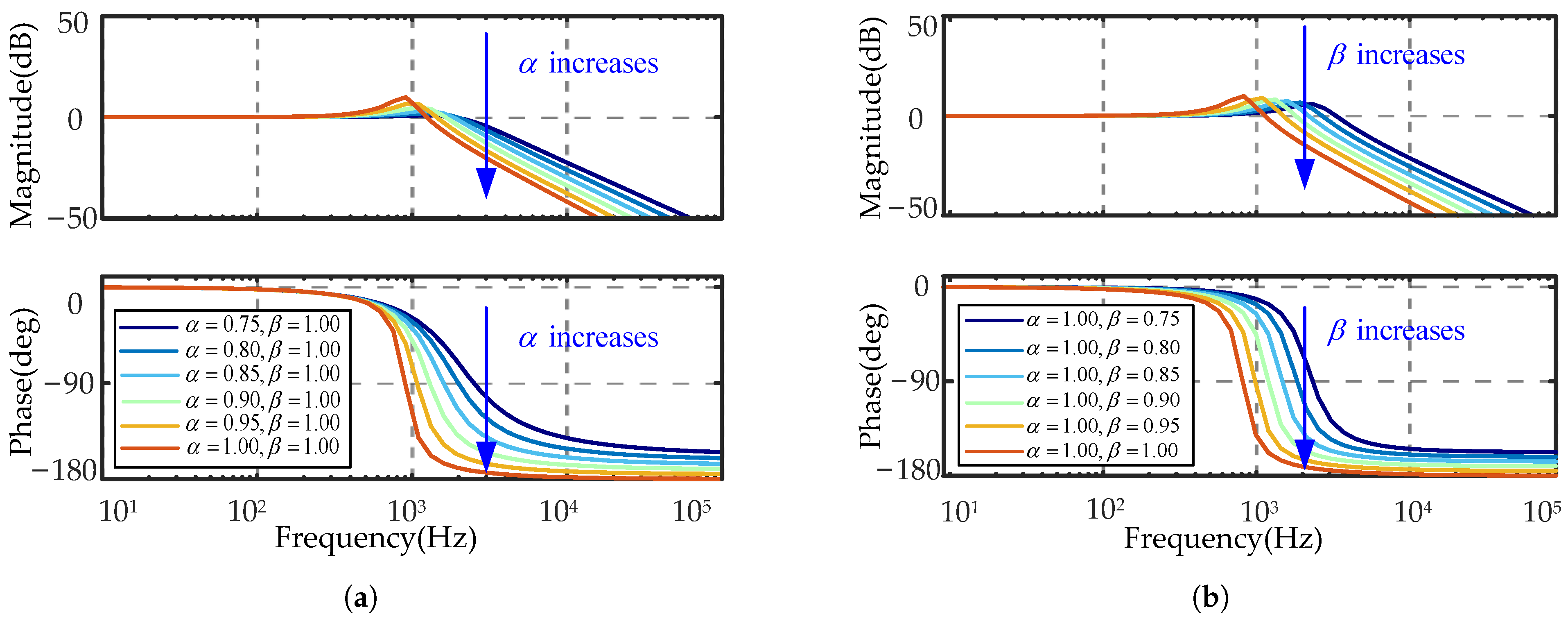
5.1. Simulation Analysis of Variations in Fractional-Order Inductor and Capacitor Orders

The system is simulated in an open-loop, no-load state to study the impact of fractional-order capacitors and fractional-order inductors on inverter performance. Initially, the effect of varying the orders of fractional-order inductors on system performance is examined, with the orders of fractional-order capacitors held constant. Subsequently, the influence of changing the orders of fractional-order capacitors on the system’s dynamic characteristics is explored, while keeping the orders of fractional-order inductors fixed. 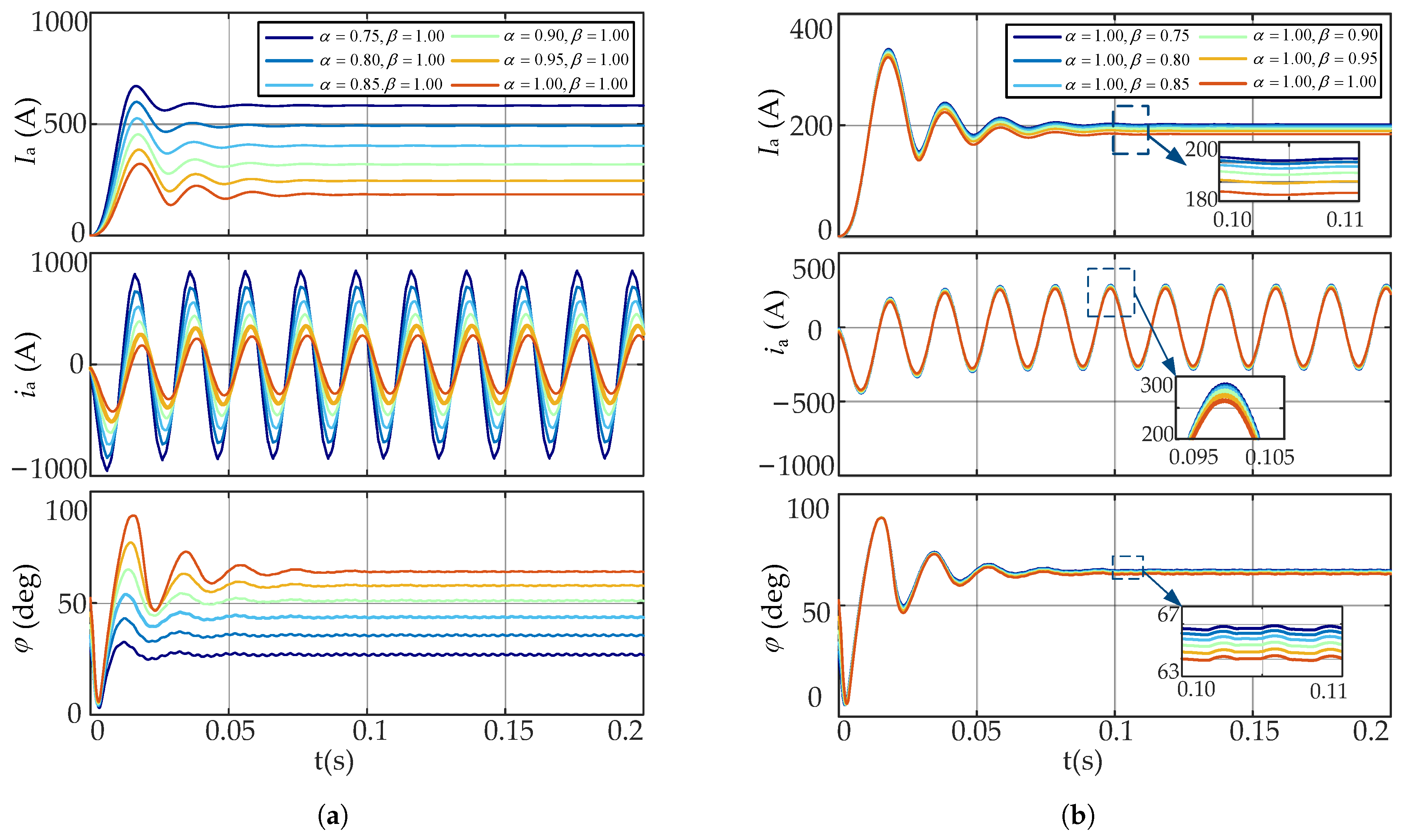Figure 12 displays the simulation results for the grid-connected current of phase A.

Figure 12a depicts the grid-connected condition as $\alpha$ rises from 0.75 to 1, with $\beta$ maintained at 1. Figure 12b illustrates the grid-connected condition as $\beta$ ranges from 0.75 to 1, with $\alpha$ maintained at 1. In the illustration, $I_{\mathrm{a}}$ signifies the RMS value of the A-phase grid-connected current, $i_{\mathrm{a}}$ depicts its instantaneous value, and $\phi$ represents the phase angle difference between the A-phase voltage and current. To facilitate the study, comprehensive simulation data are included in

Table 4. Simulation data with changing the orders of fractional-order capacitors and fractional-order inductors.

Condition	$\mathit{\alpha }/\mathit{\beta }$	${\mathit{I}}_{\mathit{a}}$ (A)	$\mathit{\phi }$ (Degree)	THD (Init.) (%)	THD (Steady) (%)
$\alpha$ increases from $0.75$ to 1 with $\beta$ fixed at 1	0.75	582.68	26.57	5.32	1.31
	0.80	492.73	35.43	6.80	1.05
	0.85	402.51	43.56	8.47	0.87
	0.90	318.75	51.12	10.12	0.74
	0.95	245.42	57.92	11.66	0.65
	1.00	183.87	64.26	13.12	0.59
$\beta$ increases from $0.75$ to 1 with $\alpha$ fixed at 1	0.75	201.24	65.86	11.97	0.63
	0.80	199.58	65.59	12.07	0.69
	0.85	197.24	65.28	12.22	0.82
	0.90	194.02	64.92	12.42	0.79
	0.95	189.75	64.54	12.71	0.63
	1.00	183.87	64.26	13.12	0.59

. The preliminary Total Harmonic Distortion (THD) readings represent the first 0.1 s, whereas the steady-state values span from 0.1 s to 0.2 s.

Figure 12 and Table 4 illustrate that while $\beta$ remains constant and $\alpha$ rises from 0.75 to 1, Ia markedly declines from 582.68 A to 183.87 A, signifying that elevated $\alpha$ values diminish the current amplitude. Furthermore, $\phi$ escalates from 26.57° to 64.26°, indicating that when $\alpha$ rises, the phase lag between voltage and current becomes increasingly significant. The initial THD climbs from 5.32% to 13.12% as $\alpha$ rises, signifying that harmonic distortion in the initial phase escalates with $\alpha$, affecting the system’s transient performance. While this elevated THD diminishes post-stabilization, it may induce current waveform distortion or exacerbate grid stress during the early phase. The total harmonic distortion (THD) diminishes from 1.31% to 0.59% in steady-state, signifying that an increase in $\alpha$ reduces the steady-state THD, thereby improving current quality. With $\alpha$ set at 1 and $\beta$ varying from 0.75 to 1, Ia exhibits a minor fluctuation, keeping within the range of 201.24 A to 183.87 A, indicating that the influence of $\beta$ on current amplitude is constrained. The variation in $\phi$ spans from 64.26° to 65.86°, suggesting that $\beta$’s influence on the system’s phase difference is negligible. Although the initial total harmonic distortion (THD) marginally rises with an increase in $\beta$, the steady-state THD continuously remains low.

In summary, $\alpha$ has a significant impact on the current amplitude, phase difference, and harmonic distortion of the grid-connected inverter. A higher $\alpha$ enhances steady-state harmonic suppression but reduces current amplitude, thereby affecting the system’s active power output. Reducing $\alpha$ appropriately can effectively decrease current phase lag, improving system efficiency and power delivery. If harmonic distortion requirements are met, performance indicators such as power factor and dynamic response can be prioritized. Considering all these factors, $\alpha =0.90$ is chosen in this study to balance harmonic suppression and output performance. In contrast, $\beta$ has minimal impact on current amplitude and phase but plays a crucial role in harmonic attenuation. If $\beta$ is set too low, high-frequency harmonic attenuation weakens, resulting in reduced filtering performance. Therefore, $\beta =0.95$ is selected in this study to ensure effective harmonic suppression without significantly affecting other dynamic characteristics of the system.

In conclusion, the selection of $\alpha =0.90$ and $\beta =0.95$ strikes a balance between harmonic control requirements, system efficiency, and dynamic performance. Furthermore, since the fractional orders of practical inductors and capacitors are typically close to one, these parameter choices also help reduce hardware implementation complexity and improve system feasibility.

5.2. Simulation Analysis of FOVSG Control

To validate the analytical results in Section 4.2 and assess the disturbance rejection capability of the proposed control strategy, two typical external disturbances were considered:

(1)

A step change in active power reference, simulating sudden variations in power commands from upper-level dispatch.

(2)

A load power disturbance, introduced to emulate abrupt changes in load demand.

5.2.1. Grid-Connected Mode

To evaluate the dynamic performance of the proposed control system, a step change in the active power reference was applied while the inverter operated in grid-connected mode. In this scenario, the grid frequency f was fixed at 50 Hz, and the inverter initially ran under nominal conditions. The inverter supplies active power to the grid, with the active power reference $P_{\mathrm{ref}}$ established at 5 kW. After one second, $P_{\mathrm{ref}}$ is increased to 10 kW. The dual-loop control parameters are shown in

Table 5. Parameter of dual-loop control.

Loop	Parameter	Value
Voltage loop	Proportional coefficient	5
	Integral coefficient	54
	Integrator order	1.12
Current loop	Proportional coefficient	15.5
	Integral coefficient	20
	Integrator order	1.08

, and the FOVSG control parameters are shown in

Table 6. Parameters of FOVSG control.

Parameter	Value
Active power droop coefficient	300
Reactive power droop coefficient	0.0001
Rated angular frequency	$100\pi$ rad/s
Rotational inertia	0.5 kg·m2
Damping coefficient	15 N·m·s/rad

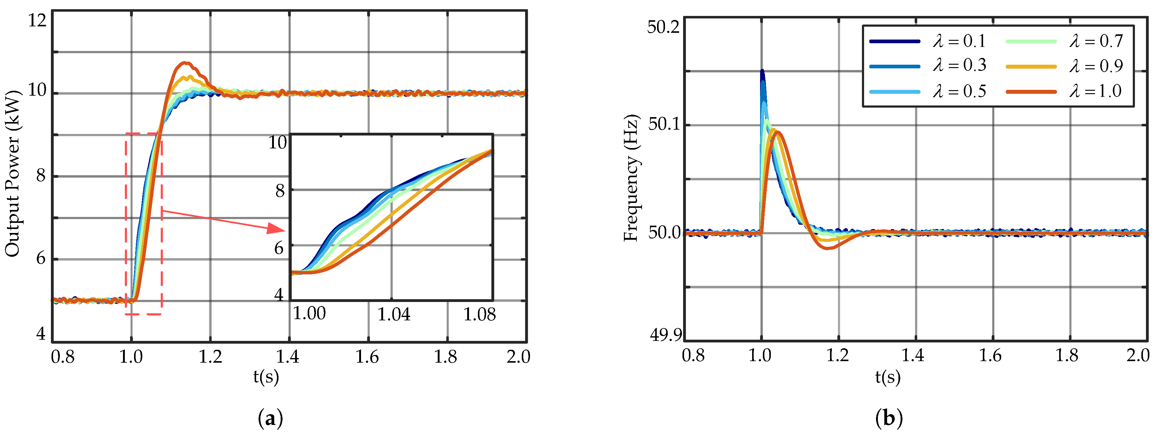
. Figure 13 depicts the power–frequency response curve for a step change in $P_{\mathrm{ref}}$ from 5 kW to 10 kW under grid-connected settings, with differing rotor orders $\lambda$ of the FOVSG.

Figure 13a illustrates that with an increase in $\lambda$, the active power response demonstrates greater overshoot and oscillations. Smaller $\lambda$ results in a steadier power response, characterized by quicker adjustments and reduced overshoot. When $\lambda =1$, the active power exhibits the largest overshoot. As $\lambda$ grows, more pronounced inertial effects result in heightened overshoot, oscillations, and diminished response speed. Figure 13b illustrates that a reduced $\lambda$ results in a rapid system response to step changes, leading to more pronounced frequency increases and greater fluctuations. When $\lambda =0.1$, the transient frequency variation is at its highest. As $\lambda$ increases, the frequency response attains a more gradual profile. At higher values of $\lambda$, the frequency curve exhibits more pronounced oscillations.

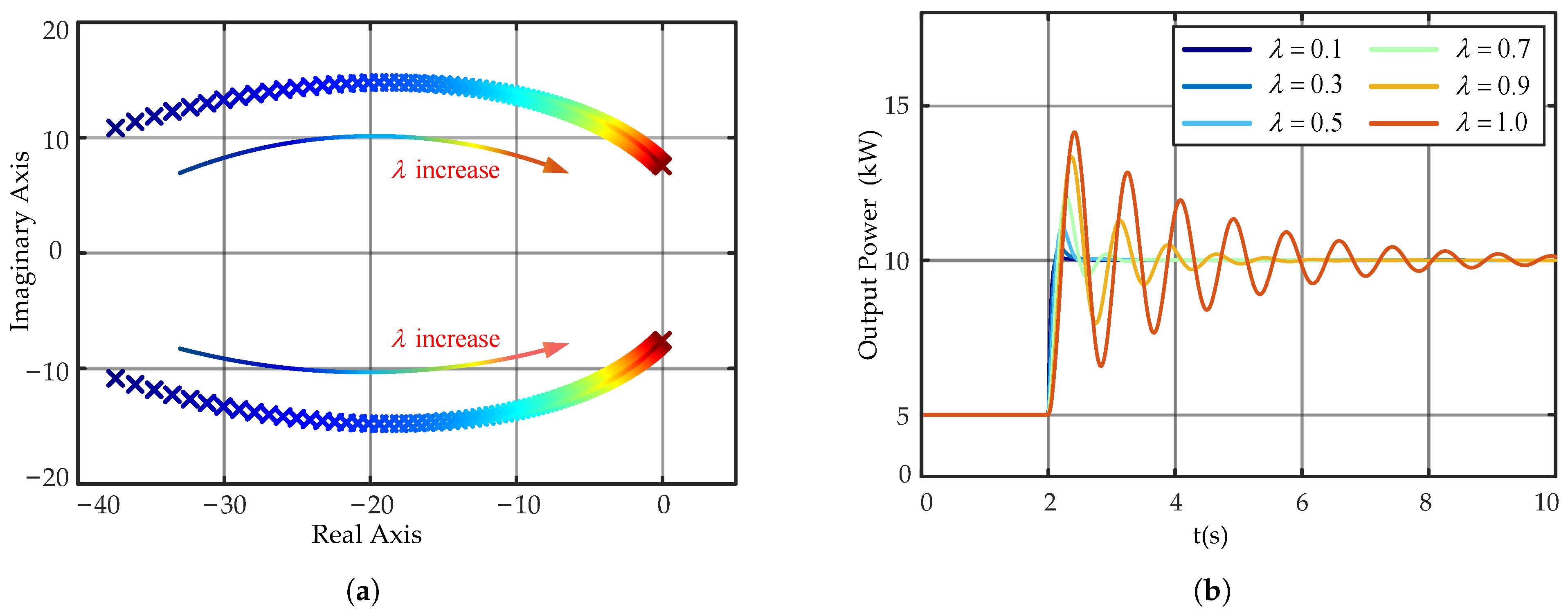
The simulation results validate the influence of $\lambda$ on the performance of grid-connected control. Reduced $\lambda$ values enhance dynamic reaction speed but compromise immediate frequency stability, whereas increased $\lambda$ values yield smoother responses but heighten the likelihood of oscillations. These findings indicate that $\lambda$ selection must equilibrate response velocity and system stability.

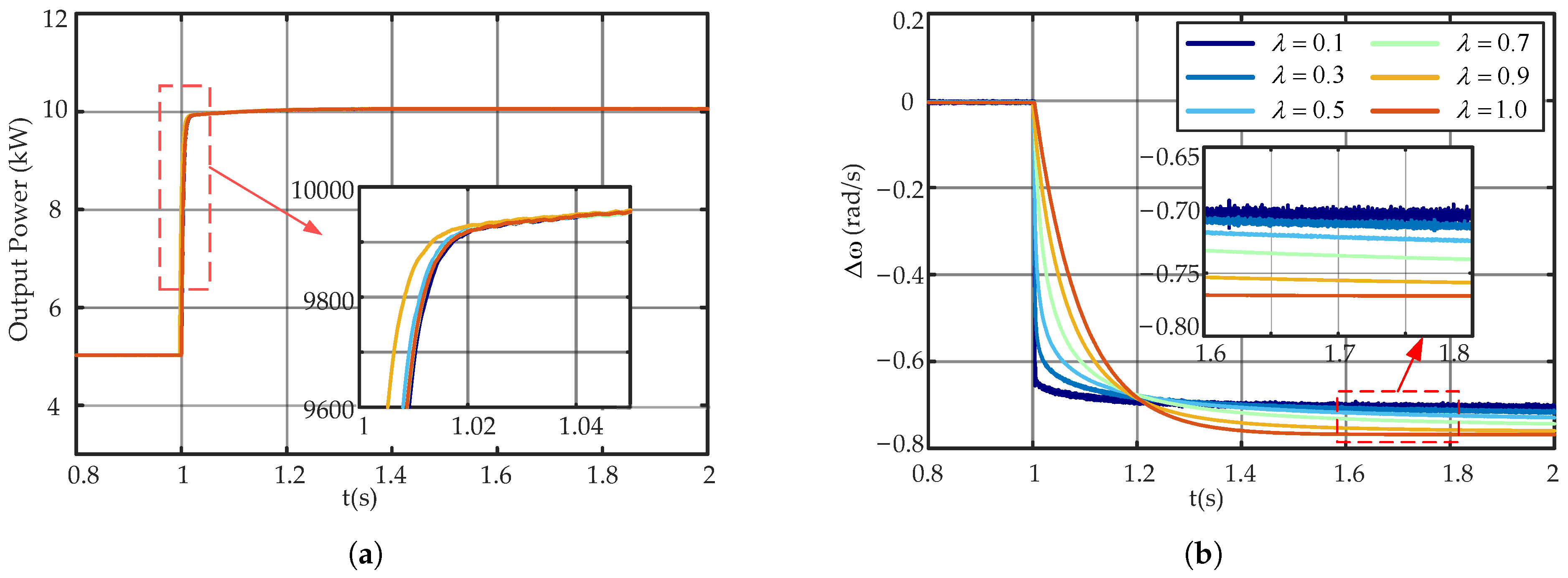
5.2.2. Islanding Mode

The following scenarios are designed to assess the impact of load power disturbance on system frequency response during islanded operation, where the load power is denoted as $P_{\mathrm{load}}$. Initially, $P_{\mathrm{ref}}$ and $P_{\mathrm{load}}$ are both 5 kW, resulting in a balanced system. After 1 s, $P_{\mathrm{load}}$ increases to 10 kW to simulate a sudden load escalation and examine its impact on system frequency response. The control parameters are unchanged as detailed in Table 5. The simulation results are shown in Figure 14.

Figure 14a illustrates the active power response under a load increase from 5 kW to 10 kW during islanding mode. It can be observed that variations in $\lambda$ have negligible impact on the power response during this disturbance, as the instantaneous increase in load power predominantly governs the power response. Figure 14b shows that for a step load disturbance of $\Delta P_{\mathrm{load}}=5\mathrm{kW}$, increasing $\lambda$ leads to a smoother transient frequency response and a lower rate of change. This confirms the theoretical insight that a higher $\lambda$ enhances virtual inertia and suppresses the rate of frequency variation. Although the steady-state frequency deviation increases with larger values of $\lambda$, the overall increment is relatively small (approximately 0.1 rad/s), which indicates that the influence on steady-state frequency remains within an acceptable range from an engineering perspective. Therefore, in islanded mode, varying $\lambda$ primarily affects the transient rate of frequency change, while its influence on the steady-state frequency deviation remains limited.

5.3. Simulation Analysis of Adaptive Rotational Inertia Control

To verify the feasibility of the proposed Adaptive Rotational Inertia Control of FOVSG (ADJ-FOVSG) strategy, in grid-connected mode, both $P_{\mathrm{ref}}$ and $P_{\mathrm{load}}$ are initially set to 5 kW, and at 1 s, $P_{\mathrm{ref}}$ suddenly increases to 10 kW. The case of Adaptive Rotational Inertia Control of FOVSG with $\lambda =1$ is selected as a reference, which corresponds to the traditional VSG with adaptive rotational inertia control (ADJ-VSG). Apart from the different $\lambda$ values, the other control parameters of the FOVSG are the same as those in the previous section, and the parameters for the adaptive rotational inertia control are shown in

Table 7. Parameters of adaptive rotational inertia control.

Parameter	Symbol	Value
Threshold for the allowable deviation in angular frequency	$D_{\omega }$	0.2 rad/s
Threshold for the allowable deviation in the rate of change of angular frequency	$D_{\mathrm{df}}$	6 rad/s2
Initial value of rotational inertia	$J_0$	0.5 kg·m2
Adjustment coefficients	$K_{\mathrm{J}1}$	0.15
	$K_{\mathrm{J}2}$	0.3
	$K_{\mathrm{J}3}$	−0.02
Inertia time constants	$T_1$	0.5
	$T_2$	0.3

.

To suppress power overshoot and reduce the transient rate of change in frequency, the fractional rotor order $\lambda$ in the ADJ-FOVSG is set to 0.7. This configuration also helps reduce fluctuations in J during adaptive control. Finally, the results are compared for four control strategies: ADJ-FOVSG, ADJ-VSG, FOVSG with $\lambda =0.7$, and VSG with $\lambda =1$, as shown in Figure 15, Figure 16, Figure 17, Figure 18 and Figure 19.

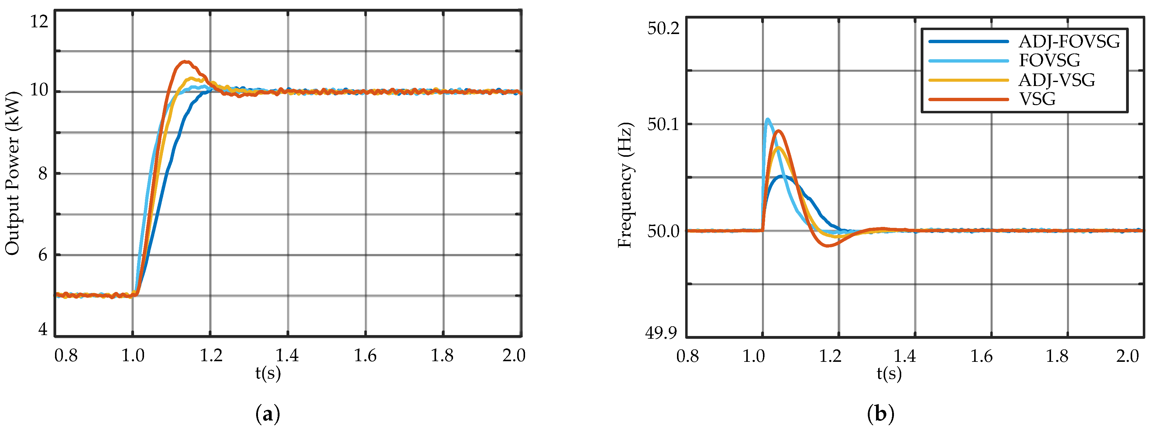
From Figure 15a, it can be observed that when $P_{\mathrm{ref}}$ undergoes a step change, the active power response under the ADJ-FOVSG control strategy is significantly faster, with the shortest settling time of only 0.19 s and no noticeable power overshoot. In contrast, the conventional VSG has a longer response time (0.29 s) and a 7.36% power overshoot, indicating poorer regulation. Figure 15b compares the frequency responses of different control strategies. The results show that ADJ-FOVSG achieves smoother frequency variations and better transient performance, with a peak deviation of only 0.059 Hz. In contrast, FOVSG has a larger deviation (0.105 Hz). This confirms that adding an adaptive regulation mechanism to FOVSG improves frequency stability and robustness during disturbances.

Table 8. Comparison of simulation experiment results.

Control Strategy	Power Regulation Time (s)	Power Overshoot (%)	Peak Frequency Deviation (Hz)
ADJ-FOVSG	0.19	0.00	0.059
FOVSG	0.20	1.16	0.105
ADJ-VSG	0.25	3.25	0.078
VSG	0.29	7.36	0.094

compares the performance metrics of all control strategies. When $P_{\mathrm{ref}}$ changes, ADJ-FOVSG effectively suppresses power overshoot. Compared to conventional VSG, ADJ-FOVSG reduces power regulation time by 34.5% and peak frequency deviation by 37.2%. Compared to the adaptive rotational inertia control in traditional VSG, ADJ-FOVSG improves regulation time by about 24% and reduces peak frequency deviation by roughly 24.4%.

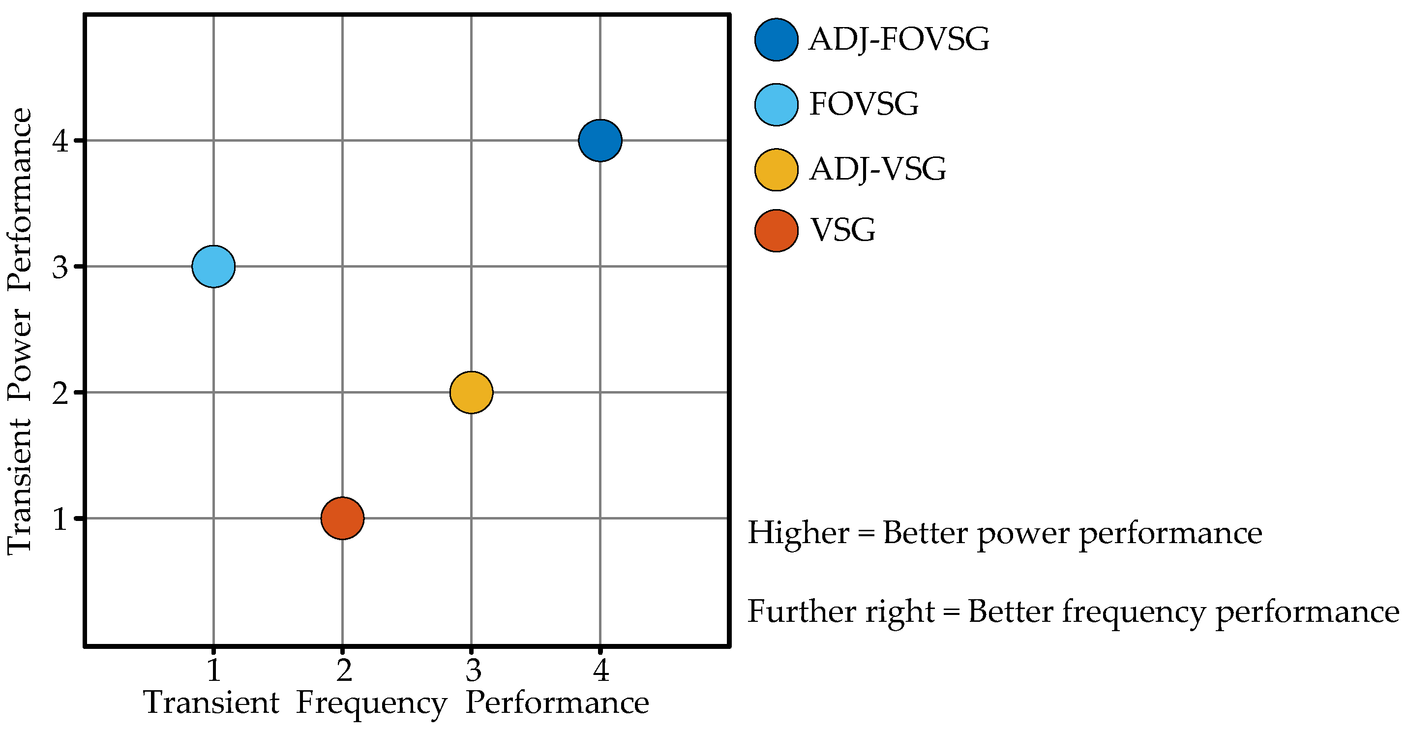
For systematic evaluation and comparison of the four control strategies’ transient performance, their results are classified into four levels in Figure 16, where higher positions indicate better power performance (less overshoot), and further right positions reflect better frequency performance (smaller rate of change).

Figure 16 presents the transient performance rankings: power performance follows ADJ-FOVSG > FOVSG > ADJ-VSG > VSG, and frequency performance follows the order ADJ-FOVSG > ADJ-VSG > VSG > FOVSG. ADJ-FOVSG clearly achieves the best overall performance, combining minimal power overshoot with reduced frequency rate of change, which confirms its superior transient characteristics. Comparatively, traditional VSG has the poorest transient power performance, and FOVSG demonstrates the weakest transient frequency response.

Figure 17 shows the variation of the rotational inertia J under the ADJ-FOVSG and ADJ-VSG control strategies. When a step disturbance occurs in $P_{\mathrm{ref}}$, causing $d\omega /dt$ and $\Delta \omega$ to exceed predefined thresholds, the adaptive control mechanism is triggered to adjust the rotational inertia and suppress frequency fluctuations. Although both strategies share the same adaptive inertia adjustment mechanism, ADJ-FOVSG exhibits superior transient performance in frequency and power regulation, as shown in Figure 15, while Figure 17 indicates that it also results in a faster and greater increase in inertia during the transient process. The observed larger and faster J increases in ADJ-FOVSG are intrinsic to the FOVSG architecture, which necessitates greater inertia modulation to counteract rapid frequency deviations. The FOVSG control structure is more sensitive to frequency variations and therefore more readily triggers inertia ramp-up during transients.

Figure 18 shows the Phase A line current waveforms under four different control strategies. With ADJ-FOVSG control, the current rises monotonically to its rated 21.44 A without overshoot. In contrast, the other three control strategies show varying degrees of overshoot, with the current briefly exceeding the rated value before gradually stabilizing. To further assess the quality of the output current during the transient process, the THD for each cycle is calculated. The THD variations of the phase A line current for the four different control strategies are shown in Figure 19. As seen in the THD variation waveform, both before the disturbance and after the transient process ends, the THD values for all control strategies remain low, indicating minimal impact on the current under steady-state conditions. During the transient period, the THD values for all strategies remain below 4%, with the ADJ-FOVSG strategy achieving the lowest maximum THD of 1.78%. This is followed by FOVSG (3.91%), VSG (2.99%), and ADJ-VSG (2.45%). These results show that the ADJ-FOVSG control strategy not only stabilizes the current response but also effectively suppresses harmonic distortion, outperforming the other strategies.

In conclusion, the introduction of adjustable parameter $\lambda$ in FOVSG provides enhanced flexibility in inertial response compared to VSG. The integration of adaptive J control into FOVSG enables dynamic inertia adjustment according to $\Delta \omega$ and $d\omega /dt$ variations during disturbances, leading to improved transient performance. By incorporating adaptive control into the FOVSG, the system can dynamically adjust J based on variations in $\Delta \omega$ and $d\omega /dt$ during disturbances, thereby enhancing transient performance. Simulation results verify that the ADJ-FOVSG surpasses ADJ-VSG, FOVSG, and VSG in transient response time, power overshoot suppression, frequency stability maintenance, and output current quality, proving its effectiveness.

6. Discussion

This paper presents a control scheme for fractional-order LC three-phase inverters, combining fractional-order virtual synchronous generator control with adaptive rotational inertia optimization. Theoretical analysis and simulation results demonstrate the scheme’s effectiveness in enhancing system stability, dynamic response, and robustness. However, despite achieving relatively ideal results, there are still challenges and limitations in practical applications. Therefore, this section will provide an in-depth discussion of the advantages and disadvantages of the proposed control strategies, challenges in hardware implementation and limitations of the study and future research directions.

(1)

Summary of the advantages and disadvantages of the control strategies.

For a clear comparison of control method characteristics,

Table 9. Summary of the advantages and disadvantages of the control strategies.

Control Strategy	Advantages	Disadvantages
VSG	The use of integer-order integrators, combined with mature algorithms and controller structures, makes the implementation straightforward and suitable for engineering applications.	Fixed parameters lead to a conflict between transient and steady-state performance.
FOVSG	Introducing the adjustable parameter $\lambda$ into the traditional VSG enhances the flexibility of the inertia response.	Fractional-order operators are approximated using filters, and the accuracy depends on the selected frequency range and filter order, which introduces implementation errors. Under disturbances, a small $\lambda$ can reduce transient power overshoot but worsens frequency performance.
ADJ-VSG	Compared with the traditional VSG, the introduction of adaptive J control enables dynamic parameter adjustment based on the system state, enhancing adaptability to disturbances.	System performance is largely limited by the structure of the adaptive algorithm and the selection of key parameters.
ADJ-FOVSG	Combining FOVSG with adaptive rotational inertia control improves the frequency response performance under small $\lambda$, while preserving the power overshoot suppression effect.	The fractional-order operator and adaptive control have inherent limitations that affect system performance and design.

summarizes the advantages and disadvantages of all four control strategies.

(2)

Challenges in hardware implementation.

In this paper, fractional-order inductors and capacitors are simulated using the Oustaloup filter to approximate their impedance functions, combined with a passive network to model their external characteristics. Although this method is feasible in terms of hardware implementation, achieving an accurate approximation of fractional-order characteristics depends on the precise combination and matching of basic components such as resistors, capacitors, and inductors. Additionally, changing the order of the fractional-order elements requires a complete network redesign. This also results in higher costs and larger physical dimensions. Developing fractional-order inductors and capacitors with simple structures and stable characteristics at the material level would greatly simplify hardware implementation.

Furthermore, as fractional-order calculus is inherently infinite-dimensional, practical implementations must use finite-dimensional approximations. The approximation accuracy depends critically on the chosen frequency range and order settings, making stable full-spectrum performance challenging to maintain. The controller’s performance depends not only on the approximation algorithm but also on the digital processor’s computational power, significantly complicating practical implementation.

(3)

Limitations of the study and future research directions.

This study validates the control strategies through theoretical analysis and numerical simulations. However, the lack of experimental verification limits the assessment of the controller’s performance under realistic grid conditions. Future work will focus on hardware-in-the-loop (HIL) testing to evaluate practical performance.

Although proposing a fractional-order LC inverter dual-loop control structure, this work lacks systematic comparison with conventional structures. Future research should investigate this strategy independently, examining how different-order decoupling configurations affect dynamic response and steady-state performance under fractional-order modeling, to optimize control structures.

While this study has demonstrated the effectiveness of the proposed control strategy under current disturbance conditions, the impact of uncertainties from actual external disturbances has not been considered. Future research could further investigate the system’s robustness against different disturbance types, particularly examining how variations in magnitude and duration affect performance, thereby enhancing the control strategy’s practicality and adaptability.

This study implements fractional-order operators using the FOTF toolbox. As operator accuracy critically impacts controller performance, developing more precise and robust approximation methods should enhance dynamic behavior and numerical stability.

7. Conclusions

This paper investigates the fractional-order characteristics of inductors and capacitors based on fractional-order calculus theory and proposes a fractional-order LC three-phase inverter topology. The mathematical model of the inverter is derived in both the three-phase stationary and the synchronously rotational coordinate systems. Additionally, a fractional-order decoupled voltage-current dual-loop control strategy is developed, incorporating the FOVSG control strategy within the power control loop, along with adaptive rotational inertia control to enhance transient performance. The proposed model and control approach are validated through theoretical analysis and simulation experiments. The findings of this research are as follows:

(1)

The fractional-order characteristics of inductors and capacitors have a significant impact on inverter performance, with the fractional-order order having a particularly strong influence. Fractional-order modeling offers a more accurate representation of inverter behavior compared to traditional integer-order models.

(2)

A mathematical model of the fractional-order three-phase LC inverter was established in both the three-phase stationary coordinate system and the two-phase rotating coordinate system. A dual closed-loop decoupling control strategy was derived to decouple the voltage and current loops by leveraging the orders of the fractional-order inductors and fractional-order capacitors, thereby improving control accuracy.

(3)

Increasing the adjustable fractional order of the rotor in the FOVSG control strategy reduces the transient frequency rate of change, thereby improving frequency stability. However, a lower rotor order suppresses active power overshoot at the cost of increased transient frequency deviations. To balance this trade-off, an adaptive rotational inertia control loop is integrated into the FOVSG, enabling real-time inertia adjustment based on grid dynamics. Experimental results demonstrate that when the reference active power changes, ADJ-FOVSG effectively suppresses power overshoot and also exhibits better transient performance in current response. Compared to traditional VSG, ADJ-FOVSG reduces the power regulation time by approximately 34.5% and decreases the peak frequency deviation by approximately 37.2%. When compared to the adaptive rotational inertia control of traditional VSG, ADJ-FOVSG improves the power regulation time by approximately 24% and reduces the peak frequency deviation by approximately 24.4%. These results confirm that the proposed ADJ-FOVSG approach achieves superior transient and steady-state performance compared to conventional strategies.