1. Introduction
Hydropower is the largest renewable electricity source in the world today. The hydropower fleet is considered quite old, where about 40% of the global fleet is 40 years old or older [
1]. The increasing installation of solar power and wind power capacity is creating new challenges for the hydropower fleet. One is intermittency, which makes the produced power output dependent on meteorological conditions [
2]. Some of this intermittency can be taken up by hydropower production [
3]. Therefore, balancing electricity sources such as hydropower will become more critical in the future [
4]. Consequently, hydropower’s ability to ramp production up and down will likely be utilized more frequently. The impact on the plant’s service life is currently unknown, but it may lead to increased maintenance efforts.
Kaplan turbines are often used in low-head hydropower applications and have adjustable runner blades, which allow for high efficiency across a wide operating range. According to the industry, some Kaplan turbines have suffered from increasing friction in their runner blade bearings located in the Kaplan hub. Some increase in friction may occur during the turbine’s lifespan without being considered to be a problem. However, there are more worrying scenarios in which the industry has installed new bearings in the turbines and the friction has increased severely over only a few years. These faults have been connected to water-lubricated bearings and are most likely connected to the design of the bearing. Eventually, this can lead to such high friction forces that the hydraulic regulation system cannot move the runner blades. This can lead to problems such that the producers can only run the turbines at fixed power outputs, which affects the flexibility and may cause a loss in revenue. To change or fix issues with the bearings, the whole runner must be lifted out of the plant, which is an expensive and time-consuming task that requires extensive planning. The industry, therefore, wants early detection of changes in friction behavior to enable better operation of the turbine to extend runner blade bearings’ service life and better planning of maintenance so it can be performed when the electricity demands are low. Today, it is rare to have sensors close to these bearings that could be used to monitor changing friction levels. Methods that could detect anomalous friction levels in these bearings from other already monitored features are, therefore, of great interest to the industry, which is why research on condition monitoring (CM) models aiming to detect anomalous friction levels in these bearings is essential.
CM and condition-based maintenance (CBM) are used to assess and predict the health of a machine. The associated costs are often justified by decreased downtime and maintenance [
5]. However, it is usually impossible to monitor everything due to high costs. Condition-based maintenance can be preferable when replacement costs are high [
6], there are no clear time intervals for failures, and failures are correlated to measurable features [
7]. Hydropower fits quite well into these criteria.
Currently, data from hydropower are often collected by a supervisory control and data acquisition (SCADA) system. Obtaining datasets with labeled faults is challenging, which is why much of the research on CM in hydropower focuses on anomaly detection, which more or less attempts to compare similar new instances to the model’s training data.
Zhu et al. developed a kernel independent component analysis and principal component analysis (KICA-PCA) model incorporating process parameters and vibration signals. The kernel independent component analysis (KICA) transforms the signals into a higher linearly separable space, and principal component analysis (PCA) is used to pick out the most essential individual components. Hotelling T
2 statistics and squared prediction error (SPE) are utilized to set a threshold based on normal or healthy training data. By comparing the statistics from new instances and examining if they are above the established threshold, anomalies can be detected [
8].
Betti et al. used a self-organizing map (SOM) to develop a key performance indicator (KPI) that compares new instances to historical data to detect anomalies. Anomalies are identified by setting a threshold value on the KPI [
9].
Furthermore, de Andrade Melani et al. suggested a hybrid system using moving window PCA for fault detection and a Bayesian network to identify specific faults. They first cluster the sensors into different fault groups, and moving window PCA is conducted on each cluster of signals. Logical values are obtained from the PCA signals from each cluster that indicate if any changes are occurring. Then, the Bayesian network indicates which cluster of signals the fault will most likely come from [
10].
Remaining useful life (RUL) models can often be complex to implement in hydropower since RUL models are typically based on data covering the entire life of a machine. Each turbine is often built for a specific location in hydropower, making them more or less unique. Moreover, large parts of the fleet were built between the 1960s and the 1980s [
1] before the SCADA systems were implemented. Because significant failures are rare, data to build ordinary RUL models are hard to obtain. A health index can be another approach to predict the machine’s behavior in the future. Jiang et al. built a composite health index using an autoencoder and an SOM network, which estimates how similar new instances are compared to the training data for the model. Long short-term memory (LSTM) was then used to predict the trend of the health index regarding future instances [
11]. This type of model can be one way to plan for maintenance without having the same amount of data that an RUL model would require.
Ahmed et al. developed a model that contains two minimum spanning trees. One global tree divides the data into clusters, which can indicate if any clusters deviate from the rest of the data. A local minimum spanning tree is also held inside each cluster to look for outliers. They can later train a classification tree from the detected outliers to detect similar faults in the data. When trained on data from a hydropower plant, a detected fault can be connected to a bearing [
12].
Pino et al. used vibration data from the startup of a turbine to develop a hidden Markov model to detect guide bearing degradation [
13].
Bütüner et al. used machine learning to predict the pressure to move the guide bearing from other process and hydraulic parameters in the SCADA system. Here, random forest provided the best results [
14].
Wang et al. used the reconstruction loss from an autoencoder that is fed with water flow and oil levels to detect inadequate lubrication of the generator guide bearing [
15].
Åsnes et al. used a one-class support vector machine model to detect high friction in the guide vane bearings by feeding the model the differential pressure and the guide vane position [
16]. This will yield only a yes or no value, which is easy for the operator to interpret. Detecting changing friction is a problem that the industry is currently looking into. However, to really evaluate the performance of friction monitoring models, a degraded system would need to be tested. This would provide insight into how sensitive the models are and need to be.
This study uses anomaly detection to develop a method for detecting anomalous friction levels in the bearings inside the hubs of Kaplan turbines. It uses operational data from two actual Kaplan turbines, each containing periods of both normal and anomalous friction conditions. Different machine-learning models and other modeling decisions have been evaluated to see how they impact the detection of anomalous friction levels inside the Kaplan runner. In more detail, the study investigates the impact of feature selection, pre-filtering of data, model selection, and the moving decision filter (MDF) impact on the final models. Metrics for model selection are also investigated as they are crucial, especially when working with a limited amount of data. Hopefully, this can help the industry to detect changed friction behaviors earlier and, therefore, be used for operation and maintenance planning.
2. Methods
The Kaplan turbine is a standard low-head turbine that can move its runner blades to achieve better efficiency for varying flows and heads. An illustration of an installed Kaplan turbine is shown in
Figure 1a. Bearings inside the turbine’s hub enable the runner blades to move and absorb the loads created by the water flow; see
Figure 1b. Here, the force from the water flow,
, is taken up by the bearings in
and
. The normal forces on the bearings are connected to the friction force
in
Figure 1c as
where
is the coefficient of friction. To regulate the runner blades, the hydraulic system needs to overcome the friction force
and the torque
from the water load. The torque
can also work in favor of the hydraulic system, depending on the point of operation and regulation direction. Changing friction coefficients will, however, affect the torque needed to regulate the system.
An increased coefficient of friction would result in a larger torque needed to move the runner blades. The torque is transferred to the runner blades by a hydraulic cylinder that is connected to all the runner blades by an internal linkage. A common way to monitor changing friction levels is the differential pressure
, which is defined as
where
and
correspond to the pressures on the hydraulic cylinder’s different sides. Natural variations in the differential pressure are connected to the power output, head, water temperature, design, power regulation, and more. The unwanted changes in the differential pressure would instead come from slow changes over time that more or less increase the overall pressure and forces required to move the runner blades.
In some cases, the industry has observed increasing differential pressures over time. To address this, glycerol is injected into the hub as a lubricant for all exposed bearings, which are otherwise water-lubricated or dry. This reduces the friction coefficient in the system and lowers the overall differential pressure. In addition to the bearings shown in
Figure 1b, there are bearings that support the axial loads on the runner blades and bearings connected to the linkage inside the hub, which enables the movement of the runner blades. The injection of glycerol will also lubricate these bearings, thereby contributing to the decrease in differential pressure. Monitoring will be important to see how long this reduction in friction will last.
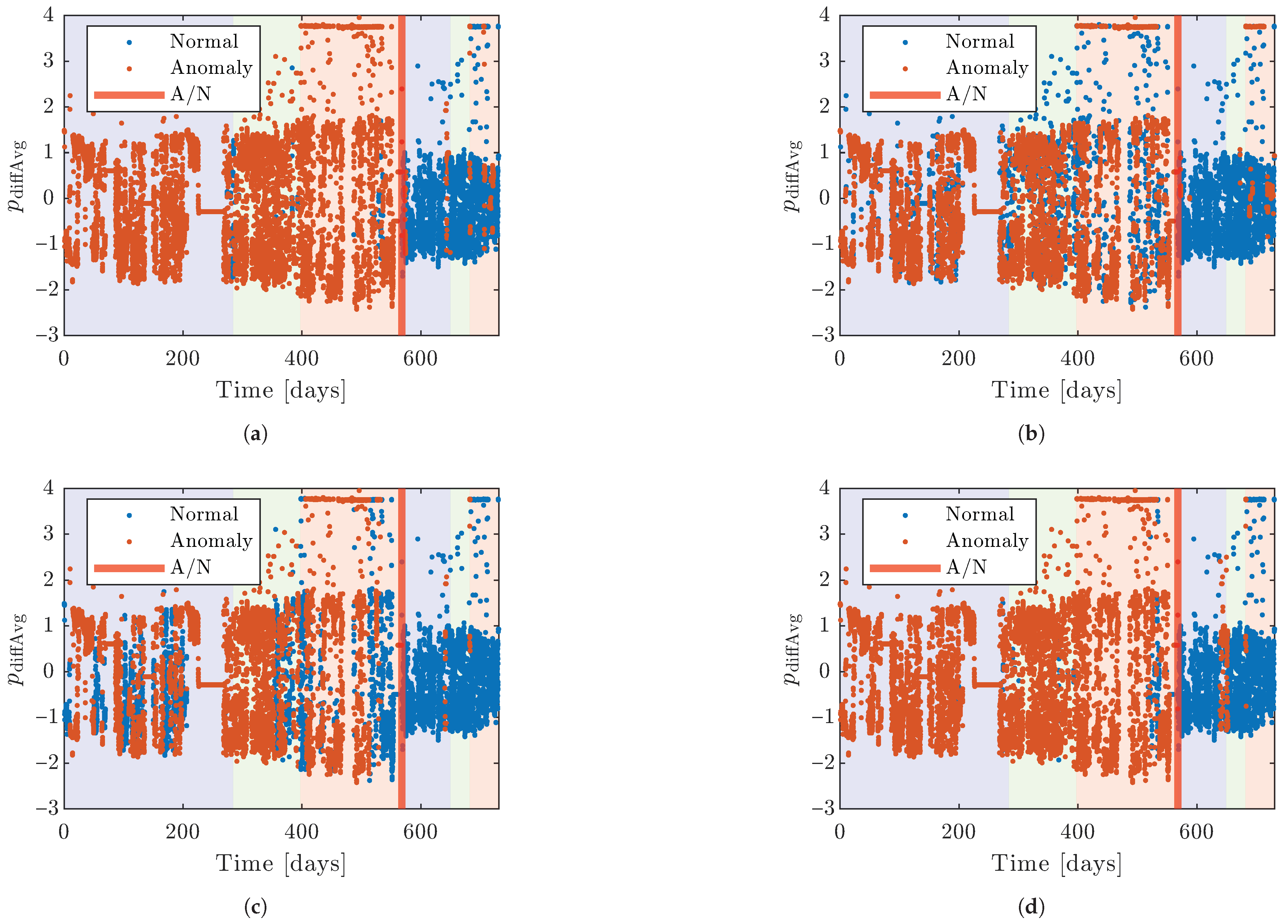
From a model perspective, injecting glycerol into the system instantly impacts the friction coefficient, allowing the data to be labeled anomalous or normal before and after the injection.
2.1. Data Acquisition
The data acquisition in this work comes from two different Kaplan turbines. The sample frequency is one sample per minute, and each feature has an average, minimum, and maximum value during each minute. The datasets are labeled according to glycerol’s presence in the Kaplan turbine’s hub during operation. In the datasets,
and
represent the pressures on the different sides of the hydraulic cylinder,
is the temperature of the hydraulic oil, and
is the system pressure in the hydraulic system. The subscripts Avg, Min, and Max denote if the value is an average, minimum, or maximum value during one minute of sampling as the original sample frequency from the SCADA system is higher than 1 sample per minute.
Table 1 summarizes the information on the different datasets.
2.2. Training, Validation, and Test Sets
The data are divided into training, validation, and test sets. The division occurs by splitting the data into specific time intervals. The first 50% of the data points is the training set, the validation set consists of the next 20%, and the test set comprises the last 30% of the points. In this way, the original order of the data points is kept, making the validation and test sets come later in time than the training sets, which hopefully will better resemble the use in the actual application. The data are divided into two parts: one without glycerol in the system, labeled as anomalous, and one where glycerol is present, labeled as normal. The anomalous and normal classes were handled separately when dividing the data, as stated above. To exemplify, this means that 50% of the anomalous and 50% of the normal data are put in the training set.
The data from both turbines are skewed as they contain more anomalous than normal data. To resolve this, all numeric results and optimizations are performed without the last points in the time series of each set of anomalous data. If nothing else is stated, the number of data points for the anomalous and normal data will be the same in evaluations regarding the performance of the models.
2.3. Features
To identify which features are the most important for anomaly detection, the features are divided into six feature sets, as seen in
Table 2. The idea of feature sets E and F is to take all available features from the data; therefore, the differential
is not included in these feature sets. Training all the models with all the feature sets provides insight into how the choice in features affects the anomaly detection performance.
2.4. Pre-Filtering
When the runner blades on the Kaplan turbine are regulated to fully closed, a mechanical stop will be reached, and the hydraulic pressures will then reach the maximum for which the system is designed. Therefore, these pressures occur during normal conditions, and the data are filtered to remove them as they may look like anomalous instances. The filtering is conducted by considering the average signals for the closing and opening pressures, and outliers are detected by considering the scaled median absolute deviation (MAD) defined as
where
X is a feature vector with
N number of samples and
. The scaled MAD is calculated for both the closing and opening pressure, and outliers are defined as values that are more than three times the scaled MAD from the median. If an outlier is detected in one of the pressures, all features from that timestamp will be replaced by the previous non-outlier value from the data.
2.5. Normalization
Normalization is conducted using the
z-score. For the data
X with a mean
and standard deviation
, the
z-score is
for single values of
x. The training and validation sets are normalized together, and the test set is normalized separately using the same mean and standard deviation from the training and validation sets.
2.6. Models
In the actual application, the models aim to detect anomalies connected to the required forces to move the runner blades. They are trained on “healthy” or normal data, considered when glycerol is present in the system. This applies to all models tested. Below is a brief explanation of the models tested in this study. The choice in models is based on their simplicity in implementation, which facilitates the implementation in real hydropower plants.
For clarity, positive predictions refer to instances predicted as anomalous, and negative predictions refer to instances predicted as normal.
2.6.1. Isolation Forest (iForest)
The isolation forest (iForest) algorithm is an ensemble of many isolation trees (iTrees), a tree model that isolates anomalies rather than profiles normal instances. Each tree has a split variable and a split position chosen at random. The tree grows until each sample has a separate leaf node. The anomaly score is then calculated by the path length where anomalies are detected near the tree’s root as they are easier to separate from the rest of the data. More information about iForest can be found in [
17]. The number of trees was set to 100, and the number of observations per tree was set to
, where
N is the number of observations.
2.6.2. Local Outlier Factor (LOF)
Local outlier factor (LOF) examines the density of points relative to surrounding neighbors. Anomalies are detected by low density, indicating greater distance to surrounding points. More information about LOF can be found in [
18]. The number of neighbors is set to
, where
n is the number of unique rows in the predictor data.
2.6.3. One-Class Support Vector Machine (OC-SVM)
One-class support vector machine is a form of unsupervised SVM, which is a kernel-based method that separates anomalies by constructing a hyperplane in a high-dimensional feature space. Points far away from the hyperplane are then considered anomalies. More about one-class support vector machine can be found in [
19]. The model uses the Gaussian kernel with a kernel scale of 1.
2.6.4. Mahalanobis Distance (MD)
Mahalanobis distance examines the distance between a sample point and a sample distribution by considering the mean and covariance of the distribution. The models tested here use the robust Mahalanobis distance.
2.7. Moving Decision Filter (MDF)
A moving decision filter is applied to the models’ anomaly scores to avoid alarms for singular anomalies in the data. The MDF is defined by two parameters: the window size and a threshold. The window size indicates how many data points should be considered in each decision. If all points in a window are greater than the predefined threshold, all points are deemed anomalous in that window. The window moves one step at a time.
Due to the many combinations of window sizes and thresholds that exist, Bayesian optimization is performed for each model and dataset to find the best combination. Bayesian optimization was chosen to reduce the number of iterations. Another benefit compared to other strategies, such as grid search, is that only the examination range for the variables needs to be defined, not the grid size. The models aim to classify the points with glycerol in the system as normal and points without glycerol as anomalous. The optimization is achieved by obtaining the highest
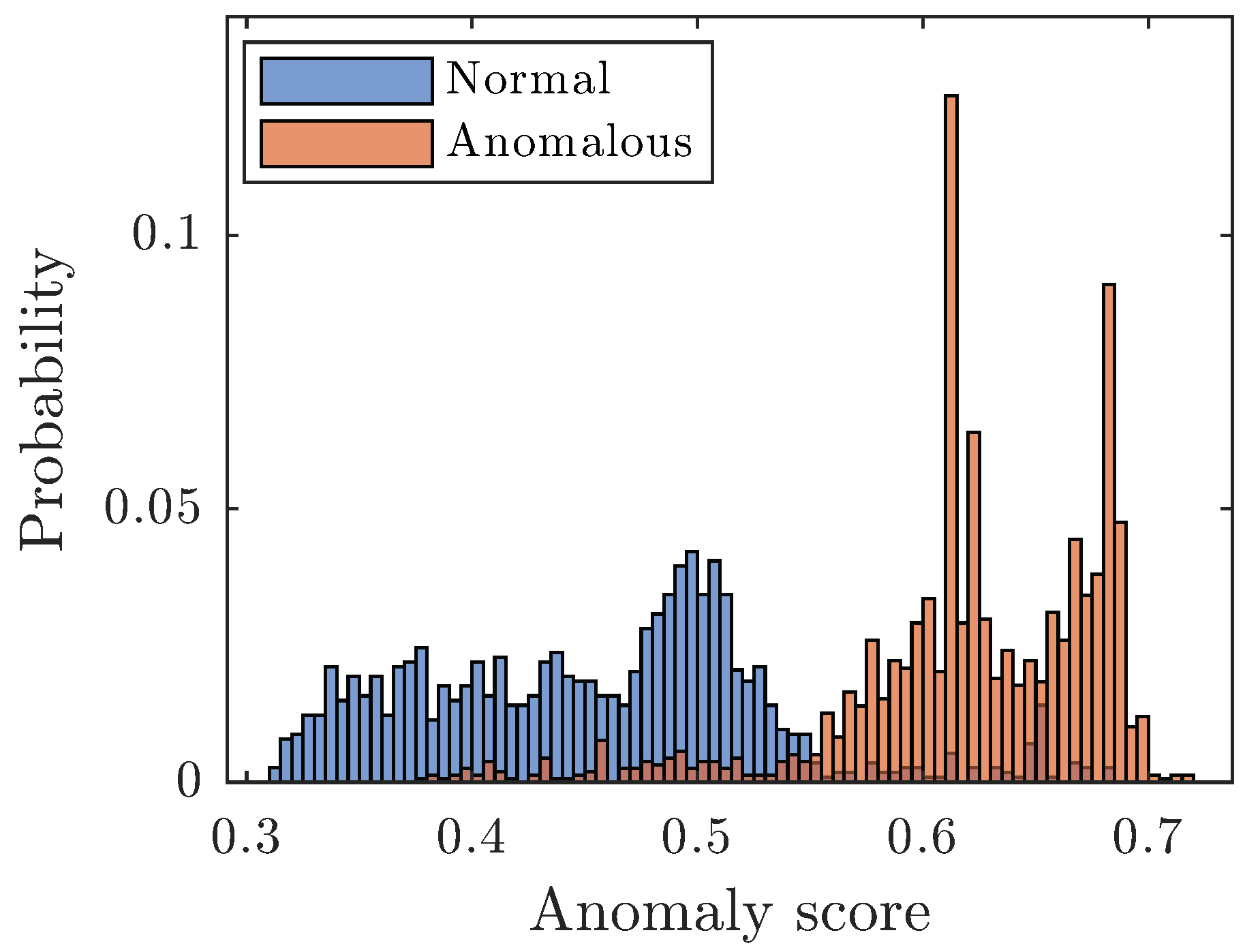
score on the validation set. The window size range is set to 1–4320, which corresponds to a time range of 1 min up to 3 days. The range of the thresholds is set individually for each model by inspecting the histograms for anomaly scores on the training and validation sets. The threshold range is then set to ensure that the best threshold will be included. As an example,
Figure 2 shows the anomaly scores for the normal and anomalous data for iForest, and here the range for the thresholds was set to 0.3–0.7. The maximum number of iterations is set to 200, but some models have overridden that with a few iterations due to parallel computing.
4. Conclusions
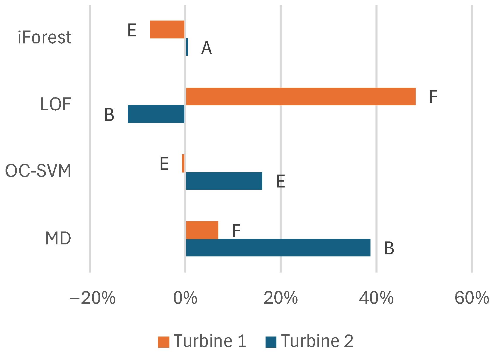
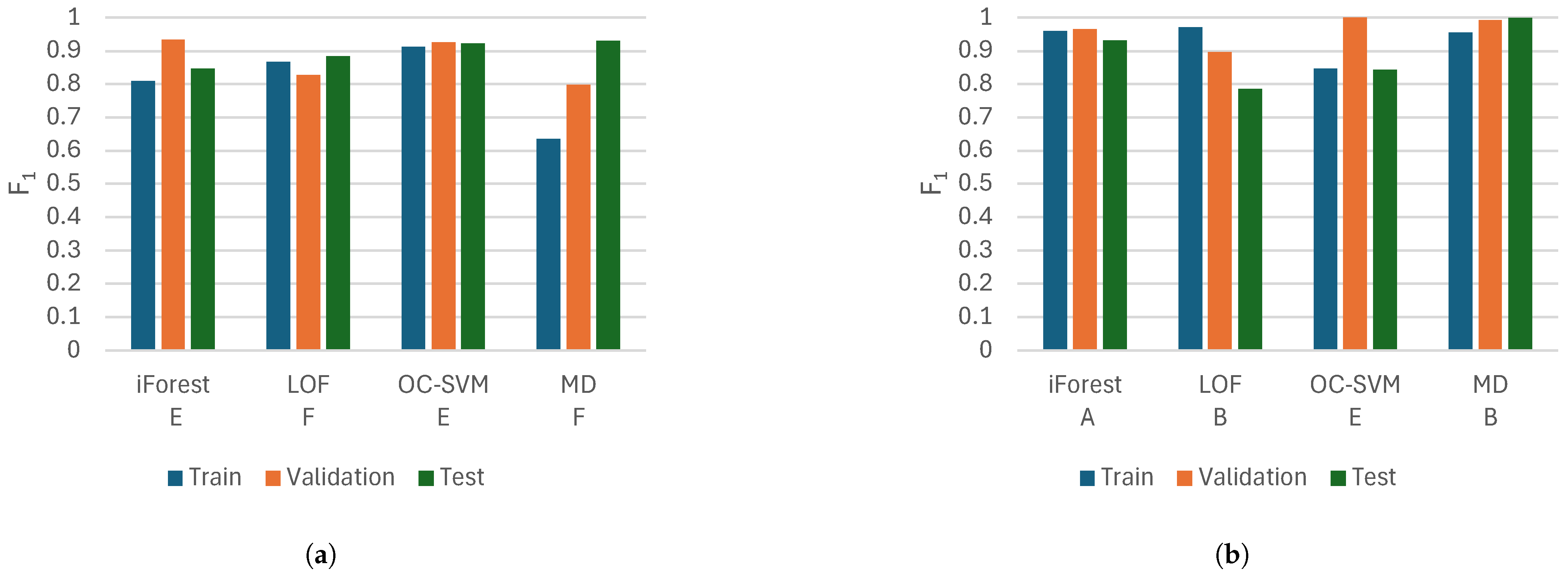
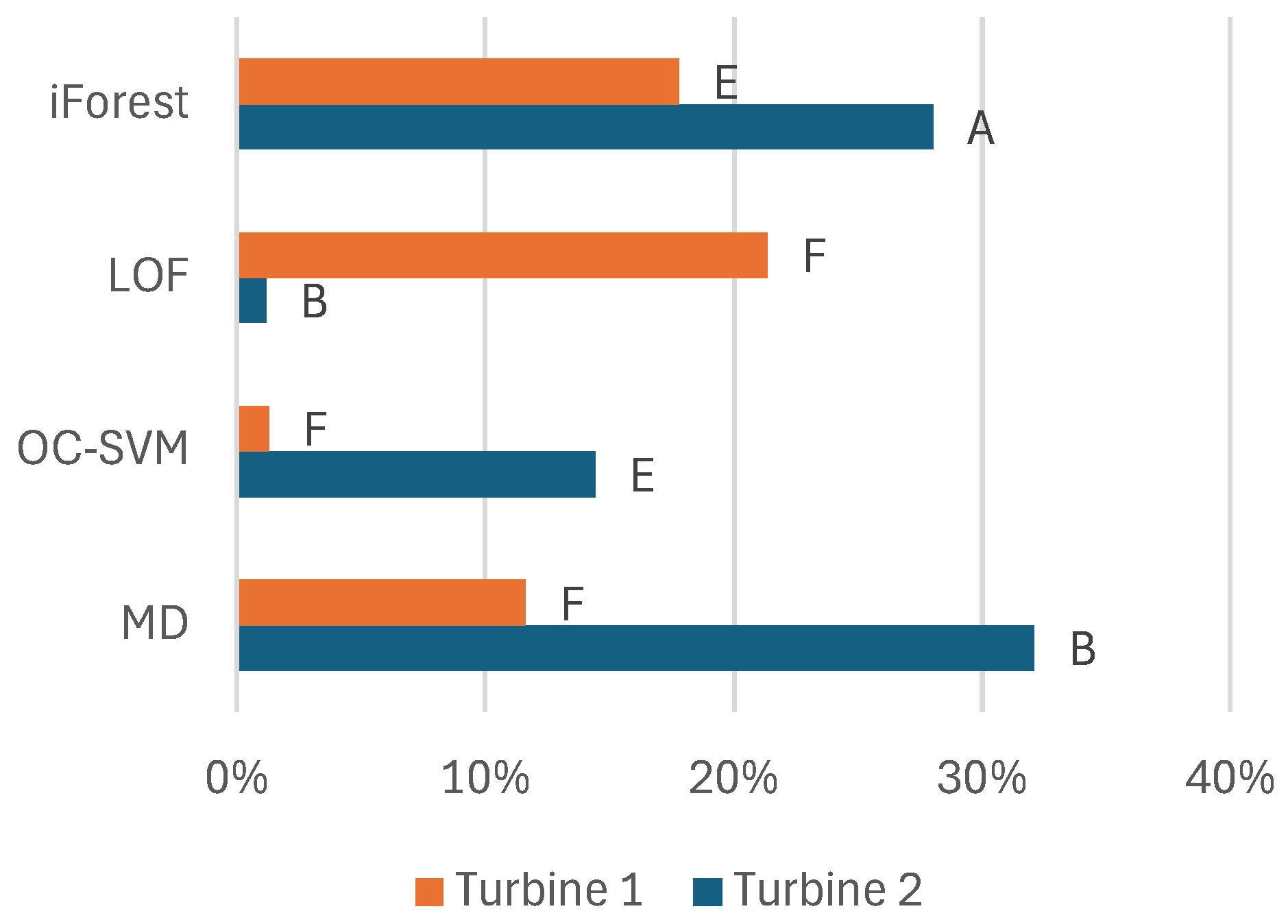
To summarize the results, we can draw conclusions about the feature set, filtering, model selection, and variations among the turbines. Regarding the features, the model benefits overall from the pressures of the raw signals instead of precalculating the differential pressure. Adding information like the minimum and maximum values during the sampling besides the average values benefits most models. Additionally, information about oil temperature adds information about this problem that benefits the models. The system pressure only adds valuable information for some models.
The pre-filtering of data using MAD benefited the models on average. However, for iForest, the drawbacks may, on the other hand, exceed the benefits, and pre-filtering could be excluded. For the other models, it is suggested that the pre-filtering of the data should be kept. However, the possible negative effects can be considered if the models lack performance.
The MDF also provides, on average, positive effects for the models. The choice in feature set also seems important to benefit from the MDF. Bayesian optimization effectively finds the best parameters for the MDF. As the net effect is positive for the best-performing models, it is suggested that the MDF should be included in the model approach for all models. As the performance of the MDF heavily depends on its parameters, the lack of optimization would probably affect the performance of the MDF negatively.
Mahalanobis distance performs best on the test set in this study. However, iForest and one-class support vector machine also perform well here and offer more stable performance over the training, validation, and test sets. The stability could be considered good as there may be few opportunities to test the models on anomalous data in many applications. This is why iForest and one-class support vector machine are suggested as good models to start with.
The data are from two Kaplan turbines; the only features separating them are the oil temperature and system pressure. Otherwise, the turbines’ issues are similar. The differences in model performance between the turbines show that we can only have an idea of which models and features to use. This modeling approach can be transferred between turbines, but it is still important to set the hyperparameters using an optimization process specific to each turbine to achieve optimal performance.
This work shows how anomaly detection can be used for friction monitoring in Kaplan turbines. It also suggests a modeling approach for friction monitoring when anomalous data exist, which can help the industry to improve the monitoring of Kaplan turbines.


