Block–Neighborhood-Based Multi-Objective Evolutionary Algorithm for Distributed Resource-Constrained Hybrid Flow Shop with Machine Breakdown

Abstract

Production scheduling that involves distributed factories, machine maintenance, and resource constraints plays a crucial role in manufacturing. However, these realistic constraints have rarely been considered simultaneously in the hybrid flow shop (HFS). To address this issue, a distributed resource-constrained hybrid flow shop scheduling problem with machine breakdowns (DRCHFSP-MB) is studied. There are two optimization objectives, i.e., makespan and total energy consumption (TEC). To solve the strongly NP-hard problem, a mathematical model is established and a block–neighborhood-based multi-objective evolutionary algorithm (BNMOEA) is developed. In the proposed algorithm, an efficient hybrid initialization method is adopted to obtain high-quality individuals to participate in the evolutionary process of the population. Next, to enhance the search capability of the BNMOEA, three well-designed crossover operators are used in the global search. Then, the convergence of the proposed algorithm is improved by utilizing eight critical factory-based local search operators combined with block–neighborhood. Finally, the BNMOEA is compared with several of the most advanced multi-objective algorithms; the results indicate that the BNMOEA has an outstanding performance in solving DRCHFSP-MB.

1. Introduction

Currently, environmental and energy crises are becoming growing worldwide problems in most countries, and companies must make a trade-off between production and green sustainable development [1,2,3]. Green manufacturing has become a crucial research topic in recent years. In addition, a complex industrial scenario gives increasing challenges to manufacturing with Industry 4.0, especially for a distributed hybrid flow shop scheduling problem (DHFSP). The DHFSP is more practical in real industrial production environments, e.g., family setup time [1] and worker fatigue [2]. Green production has been mostly ignored in the above studies; however, in actual manufacturing processes, companies achieve green production through operations such as time-sharing production [3], adjusting their processing speed [4], and switching off idle machines [5].

Many types of realistic constraints need to be considered in the manufacturing process, such as machine breakdown [6] and resource constraints [7]. Common types of resources include fuels, catalysts, and workers. Machines take up resources to process jobs. When resources are insufficient, the machine will stop processing until the current machine has finished processing before releasing the resources. In actual production settings, machine breakdowns are common. Machine breakdowns are unpredictable, and the duration of repairs varies based on the specific situation of each failure. Estimating machine failure time and repair duration is challenging, and typically, the best approach involves estimating the breakdown distribution while incorporating maintenance strategies to reduce disruptions. In the above literature, only one constraint is considered. In this paper, both resource constraints and machine breakdown are tackled.

The primary contributions of this study are as follows: (1) The DHFSP of resource constraints and machine breakdown are simultaneously considered, and a mathematical model is developed. (2) An improved initialization method is employed for quality assurance and diversity of the initial population. (3) A hybrid method with three crossover operators is employed to ensure diversity in the search space. (4) Local reinforcement based on critical factories is devised to raise the local search effect.

The remaining parts of this paper are organized as follows. The literature review of DHFSP, scheduling problems with resource constraints, and machine breakdown are introduced in Section 2. Section 3 introduces the problem under consideration and presents a mathematical model. Section 4 describes the BNMOEA in detail. In Section 5, an experimental analysis is provided. In Section 6, the conclusion and future work are summarized.

2. Literature Review

In Section 2, a brief review of the relevant literature on the DHFSP, scheduling problems with machine breakdowns, and resource constraints is presented.

2.1. Literature Review of Distributed Hybrid Flow Shop

Considering the globalized economy, the DHFSP has garnered substantial attention. This heightened interest is attributed to its remarkable efficiency, capitalizing on the diverse machining capabilities offered by factories in disparate locations. Ying and Lin addressed the DHFSP by presenting a mixed integer linear programming formulation alongside a self-tuning iterated greedy (SIG) algorithm [8]. Li et al. proposed a two-population balanced multi-objective algorithm to solve the distributed production problem of a steelmaking system considering a fuzzy processing time and a crane handling process [1]. An enhanced discrete artificial bee colony (DABC) algorithm for tackling the DHFSP was introduced by Li et al. [9]. A dynamic search process employing the shuffled frog-leaping algorithm (DSFLA) was investigated by Cai et al. to address the DHFSP, involving multiprocessor tasks [10]. Du et al. proposed a reinforcement learning approach to solve the scheduling problem of considering time-of-day tariffs and machine indicators [11]. Wang et al. proposed a variable neighborhood search method to solve a three-stage HFS [12]. Zheng et al. explored a multi-objective fuzzy DHFSP that involved fuzzy processing times and fuzzy due dates. They utilized a combination of the estimation of distribution algorithm (EDA) and iterated greedy (IG) search for their investigation [13]. Shao et al. proposed an IG algorithm incorporating a multi-search construction [14]. Wang et al. employed a bi-population cooperative memetic algorithm (BCMA) to tackle the DHFSP [15]. Shao et al. examined a multi-objective DHFSP and proposed a multi-objective evolutionary algorithm based on multi-neighborhood local search (MOEALS) [16]. Li et al. proposed a hybrid algorithm combining the whale optimization algorithm (WOA) and local search heuristics to solve a batch-delivered DHFSP [17]. Wang and Wang developed a cooperative memetic algorithm (CMA) that incorporates a reinforcement learning (RL)-based policy agent [18]. Lu et al. addressed the DHFSP by combining the advantages of genetic operators and iterative greedy algorithms [19]. Shao et al. put forward a network memetic algorithm (NMA) to solve the DHFSP with workers and energy constraints [20]. Meng et al. formulated mixed-integer linear programming (MILP) models and a constraint programming (CP) model [21]. Lei et al. introduced a multi-class teaching–learning-based optimization (MTLBO) approach aimed at concurrently minimizing both the makespan and maximum tardiness [22]. Gholami et al. examined the DHFSP involving multiprocessor tasks and introduced a solution approach combining conditional Markov chain search (CMCS) and a hybrid Q-learning–local search algorithm [23].

2.2. Scheduling Problem with Machine Breakdown

Considerable effort has been devoted to investigating machine breakdowns in the context of scheduling problems. Gholami et al. addressed HFSP that involves sequence-dependent setup times (SDSTs) and machines experiencing stochastic breakdowns [24]. Zandieh et al. devised an Immune Algorithm (IA) to address HFSP encompassing SDSTs and machines subjected to stochastic breakdowns [25]. Safari et al. introduced an algorithm for an irrecoverable process shop state where job processing after preventive maintenance restarts from the initial stages [26]. Wang et al. proposed a decomposition-based approach which divided the problem into sub-problems to solve flexible flow shops considering machine breakdowns [27]. A two-stage HFSP in the presence of machine breakdowns was investigated by Mirabi et al. [28]. Wang et al. introduced a fuzzy logic-based hybrid estimation of distribution algorithm (FL-HEDA) for handling discrete permutation flow shop problems (DPFSPs) under machine breakdown conditions [29]. Adressi et al. suggested GA- and SA-based heuristics to address the group scheduling problem within a no-wait flexible flow shop setting [30]. Fazayeli et al. developed an efficient hybrid algorithm by combining GA- and SA- based meta-heuristics to address this problem [31]. Seidgar examined two-stage assembly flow shop problems (TAFSPs) while accounting for machine breakdowns [32]. Han et al. introduced a multi-objective evolutionary robust algorithm to address scheduling problems in a blocking lot-streaming flow shop (BLSFS) environment [33]. Tadayonirad et al. studied a two-stage assembly-based robust scheduling flow shop with random machine breakdowns [34]. Marichelvam et al. introduced a hybrid approach that combines the Firefly Algorithm (FA) with the VNS algorithm to address a time-uncertain flow shop scheduling problem and machine breakdowns [35]. Seidgar et al. considered random machine breakdowns and the two-stage assembly flow shop problem in their investigation [36]. Branda et al. solved a flow shop scheduling problem characterized by machines not continuously available throughout the planning horizon. The periods of unavailability were caused by random faults [37]. Abtahi et al. introduced a predictive robust and stable approach to tackle a two-machine flow shop scheduling problem involving machine disruptions and uncertain job processing times [6].

2.3. Scheduling Problem with Resource Constraints

Resource constraints have garnered considerable attention in the scheduling field. Li et al. proposed a multi-dimensional co-evolutionary algorithm to solve a multi-objective resource-constrained flexible flow shop with robotic transportation [38]. Leu and Hwang used a search-based genetic algorithm to determine the minimum completion time, considering both resource constraints and mixed production scenarios [39]. Jarboui et al. introduced a combinatorial particle swarm optimization (CPSO) algorithm to address the multi-mode resource-constrained project scheduling problem (MRCPSP) [40]. Behnamian et al. proposed a max–min weighting approach to solving the multi-model resource-constrained scheduling problem [41]. Rajkumar et al. introduced a greedy randomized adaptive search procedure (GRASP) algorithm for addressing FJSP while considering resource constraints [42]. Cheng et al. formulated a resource-constrained two-machine scheduling problem to identify a feasible re-development sequence that minimizes the makespan [43]. Lin et al. introduced a multi-level GA incorporating correlated re-entrant possibilities and production modes into a multi-level chromosome encoding scheme [44]. Bożejko et al. took road construction as an example and proposed two novel optimization algorithms for the problem under consideration: construction and tabu search [45]. Laribi et al. considered non-renewable resource constraints and proposed a fast solution to the resource-constrained m-machine flow shop problem [46]. Li et al. proposed a bi-population balancing a multi-objective algorithm to solve a fuzzy flexible job shop with energy and transportation [1]. Rahman et al. introduced a memetic algorithm (MA) based on GA to address resource-limited scheduling problems [47]. Costa et al. investigated an m-stage HFSP where there is a limited workforce responsible for carrying out setup operations [48]. BOUFELLOUH et al. introduced a bi-objective model that encompasses production scheduling, maintenance planning, and the optimal allocation of diverse resources for production purposes [49]. Chen et al. proposed to solve a flexible job shop with crane transportation and setup times using a genetic programming-based cooperative evolutionary algorithm [50]. Han et al. introduced four hybrid decomposition (HD) methods tailored for four multi-objective evolutionary algorithm hybrids (MOEAHs) [51]. These methods integrate four priority rules for machine and worker assignments. Hosseini et al. examined a two-stage production system comprising a fabrication stage followed by an assembly stage. They proposed a novel MILP model to address this scenario [7]. Hasani et al. tackled optimizing a spring manufacturing plant within the scope of the discussed problem. The problem involves considerations of machine eligibility and sequence-dependent setup times [52].

2.4. Literature Analysis

It is clear from the above that there are constraints on FSP and HFSP and that many algorithms can effectively solve constraint-specific FSP and HFSP. However, there is no literature that uses algorithms to address both resource constraints and machine breakdown in the DHFSP. Therefore, this study proposes an efficient and applicable multi-objective intelligent optimization algorithm for resource constraints and machine breakdown.

3. Problem Description

The proposed DRCHFSP-MB can be divided into three parts: distributed hybrid flow shop scheduling; resource constraints; and machine breakdown. The three components are described in detail as below.

3.1. Distributed Hybrid Flow Shop Scheduling

The considered DHFSP can be described as follows: There are N jobs to be processed through L stages in F identical factories (F > 1). Each factory is considered a hybrid flow shop. Each machine is consistently available to process a job at any given time. Jobs follow a fixed processing order and can only be assigned to one machine at a time. Once a job is assigned to a machine, it cannot be reassigned to another machine subsequently. After completing the processing of a job in the initial stage, the job enters an unbounded buffer space until a machine in the next stage becomes available.

3.2. Resource Constraints

There are L stages in each factory, and there are different types of resources for each stage. Resources in different stages do not affect each other. The total number of each resource in each stage is fixed. Machines in different processing stages require different types of resources. When a job needs to be processed, an idle machine must be selected for processing, and the resources needed for that machine are not occupied. This means that the processing in an initial stage may lead to a shortage of corresponding resources for a machine in a subsequent stage. However, after the completion of processing, machines will release the resources they utilize.

3.3. Machine Breakdown

Due to the type of job, the complexity of the process, and the age of the machine, machine breakdowns are inevitable during processing. It is assumed that each machine has the same failure rate. Each machine can be repaired when it fails, and processing can continue after the repair is complete. Once a machine breaks down, it will retain its resource utilization, causing subsequent machines requiring the same resource to wait. The machine is not available at that time. The resource will only be released once the machine has been repaired. The job continues to be processed after it is repaired with no penalty for time loss or recovery. The probability of machine breakdown can be calculated by the exponential function [53], the number of failures conforms to a Poisson’s distribution, and the repair time follows a random distribution.

In the DRCHFSP-MB, two objectives (makespan and TEC) are considered. TEC incorporates energy usage for processing, energy expenditure during waiting, and energy consumption for general operations.

3.4. Notations and Parameters

Based on the provided description, the notations and parameters are defined as follows:

Indices
$j,j^{\prime }$	Index of jobs.
$s$	Index of stages.
$m$	Index of machines.
$f$	Index of factories.
$res$	Index of resources.
$r$	Index of machine processing positions.
$b$	Index of failure.
Parameters
$L$	Number of stages.
$F$	Number of factories.
$N$	Number of jobs.
$K$	Number of machines.
$R$	Number of resource types.
$H$	Number of failures.
$\alpha$	A large number.
$O_{j,s}$	The operation associated with job j at the sth position.
$M_s$	The collection of machines in the sth stage.
$p_{j,m,s}$	Processing time of job j in machine m at stage s.
$B_{j,s,f}$	The beginning time of the operation of job j in factory f during the sth stage.
$E_{j,s,f}$	The end time of the operation of the job j in factory f during the sth stage.
$B{M}_{m,r,f}$	The begin time of processing at the rth position on machine m within factory f.
$E{M}_{m,r,f}$	The end time of processing at the rth position on machine m within factory f.
$S{M}_{m,b,r,f}$	The start time of a breakdown at the rth position, involving failure b, on machine m within factory f.
$C{M}_{m,b,r,f}$	The completion time of a breakdown at the rth position, involving failure b, on machine m within factory f.
$S{W}_{m,res,r,f}$	The start time of waiting for resource res at the rth position on machine m within factory f.
$C{W}_{m,res,r,f}$	The completion time of waiting for resource res at the rth position on machine m within factory f.
$EPU$	Unit energy consumption except machine energy.
$TW{R}_{r,res,j,s,m,f}$	The wait time for resource res for job j on machine m at the rth position in stage s within factory f.
$TW{B}_{r,b,j,s,m,f}$	The duration of failure b for job j on machine m at the rth position during stage s in factory f.
$TW{U}_m$	Unit energy consumption of waiting resource of machine m.
$TB{U}_m$	Unit energy consumption of failure of machine m.
$TP{U}_m$	Unit energy consumption of processing machine m.
Decision variables
$X_{m,j,s,r,f}$	A binary variable (0/1), assigned the value 1 when job j is being processed at the rth position on machine m during stage s in factory f.
$Y_{m,j,s,r,f,res}$	A binary variable (0/1), with the value 1 when job j is being processed with resource res at the rth position on machine m during stage s in factory f.
$Z_{j,s,f}$	A binary variable (0/1), with a value of 1 when job j is in the processing stage s within factory f.
$U_{m,j,s,r,f,b}$	A binary variable (0/1), set to 1 when job j is being processed with failure b at the rth position on machine m during stage s in factory f.
The DRCHFSP-MB mathematical model can be formulated.

$$\min \{f_1,f_2\}$$

(1)

$$f_1=C_{\max }$$

(2)

$$f_2=TEC=E1+E2+E3$$

(3)

$$E_{s,j,f}\le C_{\max },s\in \{1\dots ,L\},j\in \{1\dots ,N\}$$

(4)

$$B{M}_{m,f,r}\ge 0,m\in \{1\dots ,K\}$$

(5)

$$E{M}_{m,f,r}\ge B{M}_{m,f,r},m\in \{1\dots ,K\}$$

(6)

$$B_{j,s,f}\ge 0,j\in \{1\dots ,N\}$$

(7)

$$E_{j,s,f}\ge 0,j\in \{1\dots ,N\}$$

(8)

$$E{M}_{m,f,r}\le B{M}_{m,f,r+1},m\in \{1\dots ,K\}$$

(9)

$$B{M}_{m,f,r+1}-E{M}_{m,f,r}+\alpha \times (1-X_{m,j,s,f,r})\ge 0,m\in \{1\dots ,K\},j\in \{1\dots ,N\}$$

(10)

$$S{W}_{m,res,f,r}\ge 0,m\in \{1\dots ,K\}$$

(11)

$$C{W}_{m,res,f,r}\ge 0,m\in \{1\dots ,K\}$$

(12)

$$C{W}_{m,res,f,r}\le S{M}_{m,res,f,r+1},m\in \{1\dots ,K\}$$

(13)

$$S{W}_{m,res,f,r+1}-C{W}_{m,res,f,r}+\alpha \times (1-Y_{m,j,s,f,r,res})\ge 0,m\in \{1\dots ,K\},j\in \{1\dots ,N\}$$

(14)

$$S{M}_{m,b,f,r}\ge 0,m\in \{1\dots ,K\}$$

(15)

$$C{M}_{m,b,f,r}\ge 0,m\in \{1\dots ,K\}$$

(16)

$$C{M}_{m,b,f,r}\le S{M}_{m,b,f,r+1},m\in \{1\dots ,K\}$$

(17)

$$S{M}_{m,b,f,r+1}-C{M}_{m,b,f,r}+\alpha \times (1-U_{m,j,s,f,r,b})\ge 0,m\in \{1\dots ,K\},j\in \{1\dots ,N\}$$

(18)

$${\displaystyle \sum _{f=1}^F{\displaystyle \sum _{m=1}^M{\displaystyle \sum _{r=1}^{{\lambda }_r}{X}_{m,j,s,f,r}=1,\forall j,s}}}$$

(19)

$${\displaystyle \sum _{f=1}^F{Z}_{j,s,f}=1,\forall j,s}$$

(20)

$$Zj,s,f=Zj,k-1,f,\forall j,1\le s\le L,f$$

(21)

$${\displaystyle \sum _{j=1}^N{\displaystyle \sum _{s=1}^L{X}_{m,j,s,f,r}}}\le 1,\forall m,r,f$$

(22)

$${\displaystyle \sum _{j=1}^N{X}_{m,j,s,f,r}}\ge {\displaystyle \sum _{j^{’}=1}^N{X}_{m,j,s,f,r+1}},m\in \{1\dots ,K\},j\in \{1\dots ,N\}$$

(23)

$$B{M}_{m,f,r}\le B_{j,s,f}+\alpha \times (1-X_{m,j,s,f,r}),m\in \{1\dots ,K\},j\in \{1\dots ,N\}$$

(24)

$$B{M}_{m,f,r}+\alpha \times (1-X_{m,j,s,f,r})\ge B_{j,s,f},m\in \{1\dots ,K\},j\in \{1\dots ,N\}$$

(25)

$$E{M}_{m,r,f}\le E_{j,s,f}+\alpha \times (1-X_{m,j,s,r,f}),\forall m,j,s,r,f$$

(26)

$$E{M}_{m,r,f}+\alpha \times (1-X_{m,j,s,r,f})\ge E_{j,s,f},\forall m,j,s,r,f$$

(27)

$$S{W}_{m,res,r,f}\le B_{j,s,f}+\alpha \times (1-Y_{m,j,s,r,f,res}),\forall m,j,s,r,f,res$$

(28)

$$S{W}_{m,res,r,f}+\alpha \times (1-Y_{m,j,s,r,f,res})\ge B_{j,s,f},\forall m,j,s,r,f,res$$

(29)

$$C{W}_{m,res,r,f}\le E_{j,s,f}+\alpha \times (1-Y_{m,j,s,r,f,res}),\forall m,j,s,r,f,res$$

(30)

$$C{W}_{m,res,r,f}+\alpha \times (1-Y_{m,j,s,r,f,res})\ge E_{j,s,f},\forall m,j,s,r,f,res$$

(31)

$$S{M}_{m,b,r,f}\le B_{j,s,f}+\alpha \times (1-U_{m,j,s,r,f,b}),\forall m,j,s,r,f,b$$

(32)

$$S{M}_{m,b,r,f}+\alpha \times (1-U_{m,j,s,r,f,b})\ge B_{j,s,f},\forall m,j,s,r,f,b$$

(33)

$$C{M}_{m,b,r,f}\le E_{j,s,f}+\alpha \times (1-Um,j,s,r,f,b),\forall m,j,s,r,f,b$$

(34)

$$C{M}_{m,b,r,f}+\alpha \times (1-U_{m,j,s,r,f,b})\ge E_{j,s,f},\forall m,j,s,r,f,b$$

(35)

$${\displaystyle \sum _{m=1}^K{\displaystyle \sum _{r=1}^{{\lambda }_r}{X}_{m,j,s,r,f}}}=Z_{j,s,f}\le 1,\forall j,s,f$$

(36)

$${\displaystyle \sum _{j=1}^N{\displaystyle \sum _{s=1}^L{Y}_{m,j,s,r,f,res}}}\ge Y_{m,j^{’},s,r,f,res},\forall m,r,f,res$$

(37)

$${\displaystyle \sum _{j=1}^N{\displaystyle \sum _{s=1}^L{Y}_{m,j,s,r,f,res}}}\le 1,\forall m,r,f,res$$

(38)

$$E1={\displaystyle \sum _{m=1}^K{\displaystyle \sum _{r=1}^{{\lambda }_r}{\displaystyle \sum _{f=1}^F(E{M}_{m,r,f}-B{M}_{m,r,f}}}})\times TP{U}_m,\forall m,r,f$$

(39)

$$E2={\displaystyle \sum _{j=1}^N{\displaystyle \sum _{m=1}^K{\displaystyle \sum _{s=1}^L{\displaystyle \sum _{f=1}^{F}TW{R}_{r,res,j,s,m,f}\times TW{U}_m}}}}+TW{B}_{r,b,j,s,m,f}\times TB{U}_m,\forall r,res,b$$

(40)

$$E3=EPU\times C_{\max }$$

(41)

Equations (1)–(3) illustrate that the objectives are to minimize makespan and total energy consumption. Equation (4) describes that the makespan is related to the completion time of each factory. Equation (5) ensures each job has a start time that corresponds to the actual production. Equation (6) ensures that the time at which processing of the job ends is larger than or equal to the time at which processing of the job begins. Equations (7) and (8) guarantee positive time for each operation. Equations (9) and (10) ensure that the start time of the next job processing should be later than the completion time of the previous job. Equations (11)–(14) represent the relationship between resources and machine processing. Equations (15)–(18) represent the relationship between machine breakdown and machine processing. Equations (19) and (20) mean that each operation can only be processed on one machine in one factory. Equation (21) shows that the same factory should be selected for each operation on the same job. Equations (22) and (23) ensure that the first available position on the machine for each operation of processing is used. Equations (24)–(27) establish the connection between the positions of machine processing and the operations assigned to them. Equations (28)–(31) create the relationship between waiting for the resource and the assigned operations. Equations (32)–(35) establish the correlation between machine breakdowns and the operations they are assigned. Equation (36) guarantees that a factory could be selected for each job. Equations (37) and (38) ensure the connection between process priority and the resources within the same stage. Equations (39)–(41) represent processing energy, waiting energy, and other energy.

3.5. Problem-Specific Example

A Gantt chart example can be utilized to explain the interplay of resource constraints and machine breakdowns within the DHFSP context. The example encompasses ten jobs, twelve machines, two stages, and two factories. As shown in Figure 1, both factory 1 and factory 2 are equipped with six machines each. Within each factory, there are three resource types established. The aggregate amount of each resource for every phase within each factory is fixed at two units. The resource requirements for each processing machine in the factory are outlined in Table 1. The number 1 signifies that machine processing necessitates this resource type, while 0 indicates the absence of such a requirement. Importantly, each resource can accommodate a maximum of two units concurrently. The processing times for individual jobs are delineated in Table 2. When a machine experiences a breakdown, it enters a fault state and continues to occupy resources until it is repaired. Finished jobs are processed before resources are released.

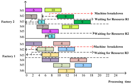
Figure 1. An example of DRCHFS-MB (rectangle with different colors represent different jobs).

Table 1. Types of resources required for the machines.

Factory	Stage	Machine	Resource Type
			R1	R2	R3
1	1	M1	1	0	1
	1	M2	0	1	1
	1	M3	1	0	1
	2	M4	0	1	0
	2	M5	1	1	1
	2	M6	0	1	0
2	1	M1	1	0	1
	1	M2	1	1	0
	1	M3	1	1	1
	2	M4	0	1	1
	2	M5	1	1	1
	2	M6	0	1	0

Table 2. Processing time.

Stage	Job
	J1	J2	J3	J4	J5	J6	J7	J8	J9	J10
1	5	5	5	5	5	5	3	2	4	5
2	5	5	5	5	5	5	3	2	4	5

In Figure 1, the sequence {J₁, J₂, J₃, J₄, J₅, J₆, J₇, J₈, J₉, J₁₀} signifies the order in which jobs are introduced into the factory for processing. Obviously, J₈ completes its initial processing stage by time 6, but the second stage of processing was not started until time 7. This delay is attributed to machine 4 and machine 5 in the second stage of factory 2 requiring one unit of resource R₃ for processing. As a result, the operation of machine 6 must wait for the completion of the processing of machine 4 and the release of 1 unit of resource R₃ before J₈ can proceed. Furthermore, J₉ should be processed at time 5. However, a machine breakdown occurred at that moment, impeding processing until the machine underwent repair. Consequently, the processing of J₉ could only commence at time 9. The discrepancy of 4 time units between these instances corresponds to the duration of the machine breakdown.

3.6. Problem-Specific Properties

Definition 1. 

Critical factory (denoted as f_key) is the factory that has the longest completion time compared with all other factories.

Lemma 1. 

C_max can only be reduced by reducing the completion time of a critical factory (if there is only one factory).

Proof. 

To prove the correctness of the lemma, assuming that the completion time of the non-critical factory is reduced, it can be seen through Equation (42) that the total completion time is related to the factory with the maximum completion time, which is called the critical factory. Therefore, C_max must be unchanged. If Equation (42) demonstrates a reduction in the total completion time, it implies that the completion time of the critical factory must also be decreased.

$$C_{\max }=\max \left\{C_{\max }^K\right|K=1,2,\dots ,f\}$$

(42)

In Figure 2, the Gantt chart is used to explain the reduction in total completion time through critical factory operations. □

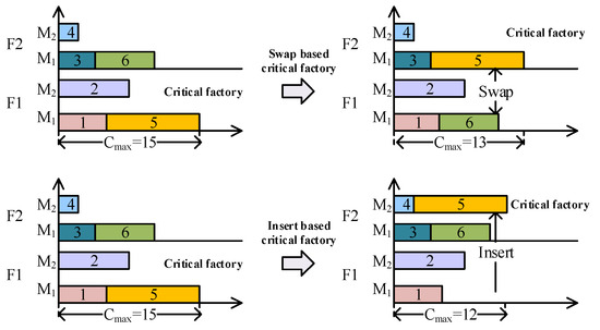
Figure 2. An example of operation of critical factory (rectangles with different colors represent different jobs).

4. The Proposed Algorithm

4.1. BNMOEA

The primary structure of the BNMOEA outlined in Figure 3 is derived from the AGEMOEAII algorithm, which is itself grounded in the Pareto frontier and is known for its strong convergence and diversity characteristics. The differences between BNMOEA and AGEMOEAII are as follows: (1) Replace the original initialization method with a hybrid initialization method. (2) Replace order crossover with three crossover operators. (3) To further enhance the local search capability, a variable neighborhood search strategy is introduced, which is centered around critical factories.

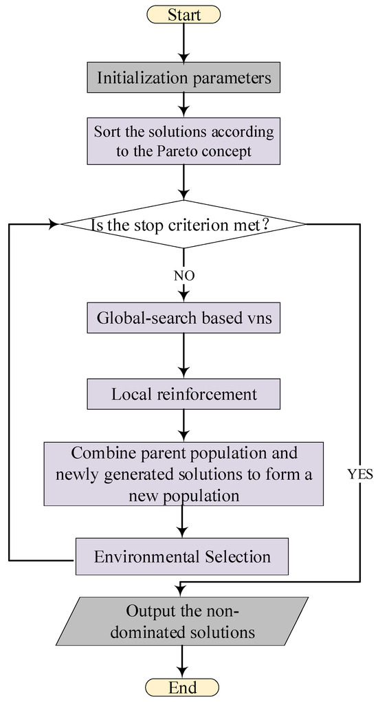
Figure 3. A framework of the BNMOEA.

4.2. Encoding

Within the algorithm under consideration, a two-dimensional vector is used to represent each solution. The vector $F=\{f_1,f_2,\dots ,f_j\}$ in the first dimension pertains to factory assignment, which guarantees that each job will be assigned to a factory. The number of jobs determines the length of the first-dimension vector. The second dimension is named the scheduling vector $\pi =\{{\pi }_1,{\pi }_2,\dots ,{\pi }_j\}$, which means that the sequence of job processing can be determined through the second dimension. The number of jobs also determines the length of the second-dimension vector.

Figure 4 and Figure 5 give a solution representation example, where the first dimension of a solution is equal to the number of factories and each location represents a factory and is associated with a dimension of values. The second dimension represents the scheduling sequence of the whole process. The scheduling sequence for each factory can be obtained. It can be seen in Figure 5 that several values represent the machine’s dependency on resources. This gives the dependence of the different machines on resources.

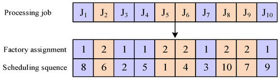
Figure 4. An example of factory assignment scheduling sequence.

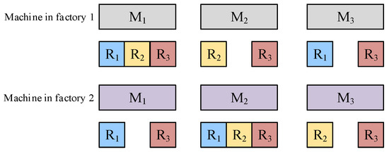
Figure 5. An example of resource constraints for machines.

The different colors indicate that the jobs are allocated to different factories, namely, J₁, J₃, J₄, J₇ and J₁₀, are processed in the first factory, whereas J₂, J₅, J₆, J₈ and J₉ are assigned to the second factory. The encoding representation also specifies the scheduling sequence of each job within each factory. The scheduling sequence obtained in Figure 4 is the overall scheduling sequence, i.e., the jobs are in the scheduling sequence of both tasks. For example, for factory 1, J₁, J₃, J₄, J₇ and J₁₀ are assigned, and the resulting scheduling sequence is then rearranged in ascending order to obtain a new processing order, which means {J₃, J₇, J₄, J₁, J₁₀}. The processing time of the job is randomly generated as an integer unit of time from 50 to 100. For instance, J₁ has an associated processing time of 55, J₇ has an associated processing time of 61, and the processing time of J₁₀ is 69. For resource constraints, the different colors of the machines represent the different factories in which they are located and each machine has different resources to match. As shown in Figure 5, machine 1 would require R₁, R₂, and R₃ in factory 1, whereas machine 1 would require R₁ and R₃ in factory 2 and R₂ is not required in factory 2. In other words, even the same machine has different dependencies on resources.

4.3. Decoding

According to the two dimensions encoding a mechanism, two problems need to be solved, i.e., which factory the jobs should be assigned to and which machine the jobs should be processed on. Considering the problems, a decoding mechanism grounded in the first-come, first-served (FCFS) principle, an earliest-available-first-served (EAFS) rule, is proposed. Firstly, in the first stage, tasks are carried out sequentially according to the order of the scheduling sequence until all machines are in the working state. It is also worth noting that when a machine is down or waiting for resources, the corresponding machine is in an unavailable state. When the machines are available, the following tasks will immediately enter the processing period. Secondly, in the after stage, according to the processing sequence of the first stage, the earlier the job is processed, the earlier it enters the after stage for processing. The specifics of the decoding mechanism are outlined in Algorithm 1.

Algorithm 1 Decoding mechanism

4.4. Population Initialization

The algorithm’s effectiveness heavily relies on the quality of the initial population. A diverse initial population of high quality may lead to faster convergence to an accurate solution. Recently, the Nawaz–Enscore–Ham (NEH) heuristic has gained significant popularity for generating high-quality initial solutions to scheduling problems. Given the outstanding capabilities exhibited by NEH, a hybrid initialization method is proposed, as shown in Algorithm 2. Each individual in the initial population contains three components, i.e., job scheduling, factory allocation, and resource assignment. The NEH heuristic is acknowledged as a highly efficient construction heuristic for HFSP that adheres to the maximum expansion criterion. By combining NEH and stochastic method, it is possible to ensure that the solutions are more diverse.

Algorithm 2 Hybrid initialization method

4.5. Global Search

Utilizing the encoding scheme as a basis, a hybrid crossover method is proposed which consists of three parts: position-based crossover, linear order crossover, and two-point crossover. The details of the global search are shown in Algorithm 3.

• Position-based Crossover

Position-based crossover for scheduling sequences: Firstly, several genes in a pair of chromosomes (parent) are randomly selected at non-contiguous positions, but both chromosomes are selected at the same position. Subsequently, offspring are produced, ensuring that the selected genes in the offspring maintain identical positions to those in the parent. Finally, determine the location of the gene chosen in the initial step within the other parent and proceed to sequentially place the remaining genes in the offspring produced during the previous step. The specific operation based on positional crossover is shown in Figure 6.

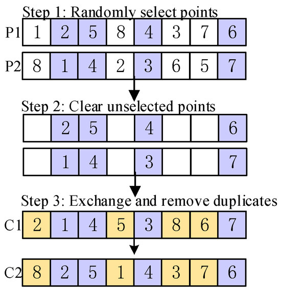
Figure 6. Details of position-based crossover.

Algorithm 3 Global search

2.

Linear order crossover

Linear order crossover for scheduling sequences is shown in Figure 7. Randomly chosen starting and ending positions in the two paternal chromosomes facilitated the copying of genes from the corresponding segment of paternal chromosome 1 to the equivalent positions in offspring 1. Subsequently, any missing genes in offspring 1 were inserted sequentially from paternal chromosome 2. Another offspring is obtained in a similar manner.

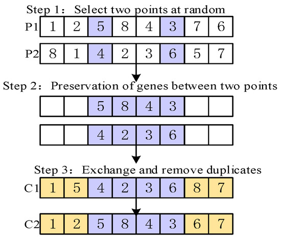
Figure 7. Details of linear order crossover.

3.

Two-points crossover

A two-point crossover involves the random selection of two crossover points within the chromosomes of individual, which is then followed by a partial exchange of genes between the chromosomes. The details of two-point crossover are shown in Figure 8.

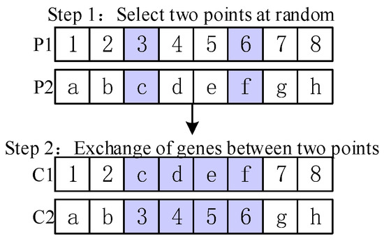
Figure 8. Details of two-point crossover.

4.6. Local Reinforcement-Based Critical Factory

In the DHFSP, the makespan is decided by the critical factory f_key with the highest completion time. Reducing the makespan of f_key is a productive method for investigating lower fitness individuals. Thus, eight sub-sequence-based operators are designed for the f_key in the local reinforcement strategy, i.e., the sub-sequence internal swap based on critical factory (SIS_cf), the sub-sequence external insert based on critical factory (SEI_cf), the sub-sequence internal insert based on critical factory (SII_cf), the sub-sequence external swap based on critical factory (SES_cf), two sub-sequence swaps between critical factory and random factory (TSS_crf), two sub-sequence insert between critical factory and random factory (TSI_crf), select points swap between critical factory and random factory (SPS_crf), and the select point insert between critical factory and random factory (SPI_crf). An illustration of the eight operators is shown in Figure 9. $\pi f_k$, $\pi f_r$ are the job scheduling sequences in the critical factory and random factory, respectively.

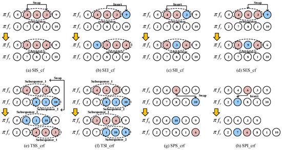
Figure 9. The details of local reinforcement.

SIS_cf: Randomly choose $\lambda$ consecutive jobs form the f_key to create the sub-sequence. The swap operator is employed on the $\lambda$ jobs in the sub-sequence jobs.

SEI_cf: Randomly choose $\lambda$ consecutive jobs form the f_key to create the sub-sequence. A random job is selected, which is the external sub-sequence. Insert the selected job into the sub-sequence.

SII_cf: Randomly choose $\lambda$ consecutive jobs form the f_key to create the sub-sequence. Insert operator is performed on the $\lambda$ jobs in the sub-sequence.

SES_cf: Randomly choose $\lambda$ consecutive jobs form the f_key to create the sub-sequence. A random job is selected, which is external to the sub-sequence. Swap the selected job with a job in the sub-sequence.

TSS_crf: Randomly select a different factory from the f_key. Then select two sub-sequences with equal length in the f_key and the chosen factory. A swap operator is employed on the two sub-sequences.

TSI_crf: Randomly select a different factory from the f_key. Then select two sub-sequences with equal length in the f_key and the chosen factory. Swap and insert operators are employed on the two sub-sequences.

SPS_crf: Randomly select a different factory from the f_key. Select a random job from each of the two factories. Swap the two jobs in different factories.

SPI_crf: Randomly select a different factory from the f_key. Select a random job in the f_key. Then insert the selected job into the chosen factory.

Eight operators are grouped into four operator sets: OS₁ = {SIS_cf, SEI_cf}, OS₂ = {SIS_cf, SEI_cf}, OS₃ = {SIS_cf, SEI_cf}, and OS₄ = {SIS_cf, SEI_cf}. To maintain offspring dispersion and enhance the quality of the solution, the four operator sets are executed using the variable neighborhood search strategy (VNS) framework. Algorithm 4 outlines the steps involved in implementing the local reinforcement strategy.

Algorithm 4 Local reinforcement-based critical factory

5. Experimental Results

5.1. Experimental Settings

To demonstrate the performance of the proposed algorithm, four algorithms are chosen from the PlatEMO [54], including NSGA-II [55], AGEMOEAII [56], CMOPSO [57], and BiGE [58]. NSGA-II is a widely used classical multi-objective optimization algorithm and has been validated in many fields with a good performance, while CMOPSO, BiGE, and AGEMOEAII are relatively new multi-objective algorithms with good performances. All comparison algorithms utilized the coding and decoding heuristics discussed in Section 4.2 and Section 4.3, respectively, to adapt to solving the problems considered. For each instance, each comparison algorithm performs 30 independent runs and the stop criterion for each run is set to 1000 iterations.

The population size for each comparison algorithm is set to 20 considering the computational cost. For fair comparisons, all parameters of the compared algorithms are set to the recommended values as in the PlatEMO platform, which are shown as follows: (1) NSGA-II: the values for the crossover probability and mutation probability are set to 0.9 and 1/n, respectively; (2) AGEMOEAII: the crossover probability is set to 1, the mutation probability is set to 1/n, and the distributed index for SBX and mutation are set to 30 and 20, respectively; (3) CMOPSO: the elite particle size is set to 10; (4) BiGE: the crossover probability is set to 1 and the mutation probability is set to 1/n.

Ying and Lin (2018) [8] provided 570 instances, which are available at http://swlin.cgu.edu.tw/data/DHFSP.zip (access on 5 October 2025). To demonstrate the performance of the BNMOEA, 27 test instances of different sizes are generated based on the instances from Ying and Lin and extended according to the constraints in this study in a random way. The 27 test instances are a combination of different jobs, stages, factories, and resources. Specifically, it is a combination of the following parameters: j = {20, 60, 100}, s = {2, 3, 4}, f = {2, 3, 4}, r = {3, 4, 5}. For example, ‘20 × 2 × 2 × 3’ means that there are twenty jobs that are to be completed in two factories, with each job requiring two processing stages, and there are three types of resources available to the machine at each stage. In addition, the processing time of each job is distributed in [50, 100] in a random way. The instances, experimental data, and codes can be downloaded at https://github.com/DATAdriving/Public_Machines.git (access on 5 October 2025).

5.2. Performance Indicators

Hypervolume (HV) [38,59,60,61,62] and inverse generational distance (IGD) [12,63,64,65,66,67] are used to evaluate the performance of the algorithm. To prove the effectiveness of the proposed algorithm, the results which are non-dominated solutions after 30 independent runs of the algorithm are taken out for comparison. In addition, because there are non-benchmarks for the problem considered, no Pareto front can be found to calculate the IGD results. Therefore, we collect all the results obtained by running the comparison algorithms for 3000 iterations and construct the Pareto front.

The relative percentage increase (RPI) was used to compare the performance of the algorithms. The specific formula is shown below:

$$RPI(C)={\displaystyle \frac{f-f_b}{f_b}}\times 100$$

(43)

where f denotes the evaluation metric of the current algorithm, while f_b represents the highest value among all current algorithmic evaluation metrics. The evaluation indicator is HV or IGD.

5.3. Parameter Setting

During the experiments, there are two main parameters including crossover and mutation probability that affect the performance of the algorithm. To demonstrate the efficient performance of the algorithm, a full analytical factorial design is performed for both parameters to select better parameters. There are five levels of each parameter in the design, as shown in Table 3.

Table 3. Parameter settings and factor levels.

Parameter	Factor Level
	1	2	3	4
pc	0.2	0.4	0.6	0.8
pm	0.2	0.4	0.6	0.8

To increase the efficiency of implementation and evaluation of experiments, the Taguchi method was widely utilized with a well-designed structure for evaluating production processes because the required number of experiments is reduced significantly [68]. For these five levels and two parameters, we generated 25 different combinations for the Taguchi experiments. The design-of-experiments (DOE) calculations were performed on 25 various combinations to compute the average HV (Ave_HV), as shown in Table 4.

Table 4. The parameter combinations and response values of DOE.

Order	pc	pm	Ave_HV
1	1	1	0.42
2	1	2	0.46
3	1	3	0.47
4	1	4	0.46
5	1	5	0.44
6	2	1	0.50
7	2	2	0.49
8	2	3	0.58
9	2	4	0.53
10	2	5	0.43
11	3	1	0.56
12	3	2	0.42
13	3	3	0.44
14	3	4	0.50
15	3	5	0.43
16	4	1	0.46
17	4	2	0.42
18	4	3	0.46
19	4	4	0.47
20	4	5	0.46
21	5	1	0.44
22	5	2	0.50
23	5	3	0.49
24	5	4	0.58
25	5	5	0.53

Figure 10 gives the trend of the two parameters. According to Figure 10, the combination of pc = 0.8 and pm = 0.4 gives the optimal indicator value. To better reflect the performance of the algorithm, the crossover probability is set to 0.8 and the mutation probability is set to 0.4.

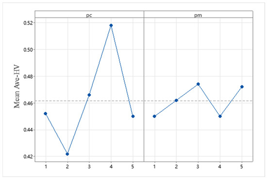
Figure 10. Trends in pc and pm parameters.

5.4. Ablation Experiments

To investigate the effectiveness of each component embedded in the proposed algorithm, including the initialization method, global search, and local search heuristics, we compared the proposed algorithm with the following three extensions: (1) the first type is the one without the proposed three crossover operators called E1; (2) the second one is the version with a random initialization approach rather than the proposed initialization approach, which is called E1; (3) the last one is the version without the local reinforcement method named E3.

Table 5 illustrates the results of the ablation comparisons for the HV values, where the first column indicates the size of the instance. The second column shows the best results collected by the four compared algorithms. The following four columns list the HV results obtained by the BNMOEA, E1, E2, and E3, respectively. The last four columns show the RPI values for the four algorithms, respectively. It can be observed that (1) the proposed BNMOEA with all the initialization, global, and local search heuristics can find all the best results for the given 27 instances; (2) the average performance shown in the last line verifies the robustness of the BNMOEA; (3) the average RPI values for E1, E2, and E3 show that the global search component contributes most to performance, and the following components are the initialization method and the local search part.

Table 5. Ablation comparison results of the HV values.

Inst	Best	HV Values				RPI Values
		BNMOEA	E1	E2	E3	BNMOEA	E1	E2	E3
20 × 2 × 2 × 3	0.7014	0.7014	0.6978	0.6961	0.6202	0.0000	−0.0051	−0.0076	−0.1158
20 × 2 × 3 × 4	0.6787	0.6787	0.6532	0.6453	0.5960	0.0000	−0.0376	−0.0492	−0.1219
20 × 2 × 4 × 5	0.6712	0.6712	0.6624	0.6667	0.6016	0.0000	−0.0131	−0.0067	−0.1037
20 × 3 × 2 × 4	0.6814	0.6814	0.6748	0.6726	0.6271	0.0000	−0.0097	−0.0129	−0.0797
20 × 3 × 3 × 5	0.6804	0.6804	0.6419	0.6445	0.5356	0.0000	−0.0566	−0.0528	−0.2128
20 × 3 × 4 × 3	0.6625	0.6625	0.6451	0.6460	0.6109	0.0000	−0.0263	−0.0249	−0.0779
20 × 4 × 2 × 5	0.6910	0.6910	0.6799	0.6781	0.5375	0.0000	−0.0161	−0.0187	−0.2221
20 × 4 × 3 × 3	0.6984	0.6984	0.6282	0.6745	0.5860	0.0000	−0.1005	−0.0342	−0.1609
20 × 4 × 4 × 4	0.6703	0.6703	0.6516	0.6528	0.6290	0.0000	−0.0279	−0.0261	−0.0616
60 × 2 × 2 × 3	0.6680	0.6680	0.6555	0.6242	0.6305	0.0000	−0.0187	−0.0656	−0.0561
60 × 2 × 3 × 4	0.6361	0.6361	0.6284	0.5739	0.5742	0.0000	−0.0121	−0.0978	−0.0973
60 × 2 × 4 × 5	0.6768	0.6768	0.6704	0.6352	0.6452	0.0000	−0.0095	−0.0615	−0.0467
60 × 3 × 2 × 4	0.6622	0.6622	0.6532	0.6106	0.6150	0.0000	−0.0136	−0.0779	−0.0713
60 × 3 × 3 × 5	0.6628	0.6628	0.6486	0.6257	0.6251	0.0000	−0.0214	−0.0560	−0.0569
60 × 3 × 4 × 3	0.6688	0.6688	0.6538	0.6150	0.6123	0.0000	−0.0224	−0.0804	−0.0845
60 × 4 × 2 × 5	0.6637	0.6637	0.6422	0.5931	0.5949	0.0000	−0.0324	−0.1064	−0.1037
60 × 4 × 3 × 3	0.6726	0.6726	0.6516	0.6291	0.6287	0.0000	−0.0312	−0.0647	−0.0653
60 × 4 × 4 × 4	0.6756	0.6756	0.6677	0.6227	0.6349	0.0000	−0.0117	−0.0783	−0.0602
100 × 2 × 2 × 3	0.6693	0.6693	0.6628	0.6159	0.6324	0.0000	−0.0097	−0.0798	−0.0551
100 × 2 × 3 × 4	0.6544	0.6544	0.6539	0.5966	0.6030	0.0000	−0.0008	−0.0883	−0.0785
100 × 2 × 4 × 5	0.6675	0.6675	0.6584	0.6146	0.6153	0.0000	−0.0136	−0.0793	−0.0782
100 × 3 × 2 × 4	0.6885	0.6885	0.6795	0.6408	0.6317	0.0000	−0.0131	−0.0693	−0.0825
100 × 3 × 3 × 5	0.6616	0.6616	0.6589	0.6173	0.6172	0.0000	−0.0041	−0.0670	−0.0671
100 × 3 × 4 × 3	0.6752	0.6752	0.6586	0.6303	0.6305	0.0000	−0.0246	−0.0665	−0.0662
100 × 4 × 2 × 5	0.6580	0.6580	0.6519	0.6009	0.6041	0.0000	−0.0093	−0.0868	−0.0819
100 × 4 × 3 × 3	0.6706	0.6706	0.6560	0.6176	0.6147	0.0000	−0.0218	−0.0790	−0.0834
100 × 4 × 4 × 4	0.6563	0.6563	0.6416	0.6079	0.5976	0.0000	−0.0224	−0.0737	−0.0894
Avg	0.6712	0.6712	0.6566	0.6314	0.6093	0.0000	−0.0217	−0.0597	−0.0919

The Friedman test and the Kruskal–Wallis one-way analysis of variance are two commonly used non-parametric test methods. To test whether the comparison results are statistically significant, both non-parametric test methods are utilized. The Kruskal–Wallis comparisons and Friedman’s test results for the HV values are illustrated in Figure 11 and Figure 12, respectively, which further verify the efficiency of the proposed components.

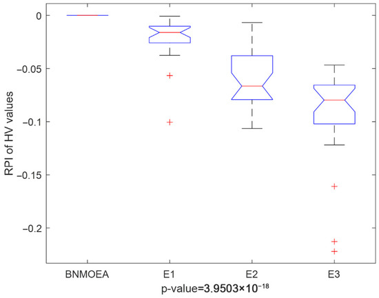
Figure 11. Kruskal–Wallis’s comparisons for the ablation experiments (HV values).

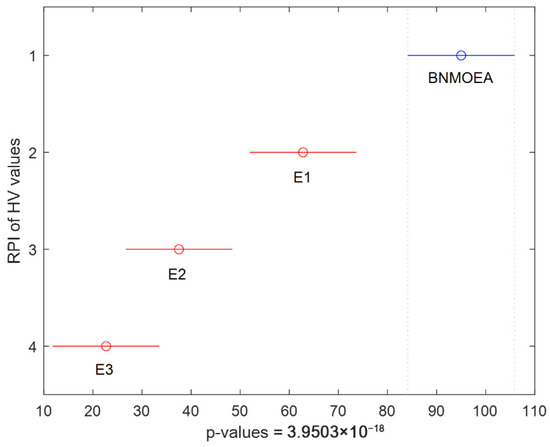
Figure 12. Friedman’s comparisons for the ablation experiments (V values).

Table 6 shows the results of the ablation comparisons for the IGD values, while Figure 13 and Figure 14 illustrate the comparison results of the IGD values obtained by the Kruskal–Wallis comparisons and the Friedman test, respectively. It can be observed that (1) considering the IGD values, the method with all three components can obtain all the best results; (2) the global search component contributes the most to the performance.

Table 6. Ablation comparison results of the IGD values.

Inst	Best	IGD Values
		BNMOEA	E1	E2	E3
20 × 2 × 2 × 3	0.0183	0.0183	0.0819	0.0646	1.0000
20 × 2 × 3 × 4	0.0147	0.0147	0.1729	0.3199	1.0000
20 × 2 × 4 × 5	0.0101	0.0101	0.2141	0.1652	1.0000
20 × 3 × 2 × 4	0.0103	0.0103	0.1069	0.1653	1.0000
20 × 3 × 3 × 5	0.1147	0.1147	0.2504	0.1769	1.0000
20 × 3 × 4 × 3	0.0147	0.0147	0.0765	0.0907	1.0000
20 × 4 × 2 × 5	0.0269	0.0269	0.1391	0.2061	1.0000
20 × 4 × 3 × 3	0.0711	0.0711	0.3292	0.3687	1.0000
20 × 4 × 4 × 4	0.0367	0.0367	0.3674	0.2548	1.0000
60 × 2 × 2 × 3	0.0870	0.0870	0.2043	1.0000	0.7915
60 × 2 × 3 × 4	0.0397	0.0397	0.4303	0.7603	1.0000
60 × 2 × 4 × 5	0.0238	0.0238	0.1687	1.0000	0.5134
60 × 3 × 2 × 4	0.0251	0.0251	0.1554	1.0000	0.9748
60 × 3 × 3 × 5	0.0109	0.0109	0.1325	1.0000	0.4452
60 × 3 × 4 × 3	0.0002	0.0002	0.0788	1.0000	0.8079
60 × 4 × 2 × 5	0.0212	0.0212	0.0493	1.0000	0.9121
60 × 4 × 3 × 3	0.0036	0.0036	0.3392	1.0000	0.7271
60 × 4 × 4 × 4	0.0112	0.0112	0.1511	1.0000	0.5732
100 × 2 × 2 × 3	0.0043	0.0043	0.1935	1.0000	0.8946
100 × 2 × 3 × 4	0.0031	0.0031	0.0608	1.0000	0.8149
100 × 2 × 4 × 5	0.1570	0.1570	0.2476	0.8717	1.0000
100 × 3 × 2 × 4	0.1061	0.1061	0.2052	1.0000	0.8736
100 × 3 × 3 × 5	0.0160	0.0160	0.0980	0.6622	1.0000
100 × 3 × 4 × 3	0.0138	0.0138	0.2846	0.8844	1.0000
100 × 4 × 2 × 5	0.0803	0.0803	0.2263	0.9097	1.0000
100 × 4 × 3 × 3	0.0125	0.0125	0.1975	0.9981	1.0000
100 × 4 × 4 × 4	0.2242	0.2242	0.2877	0.8609	1.0000
Avg	0.0429	0.0429	0.1944	0.6948	0.9010

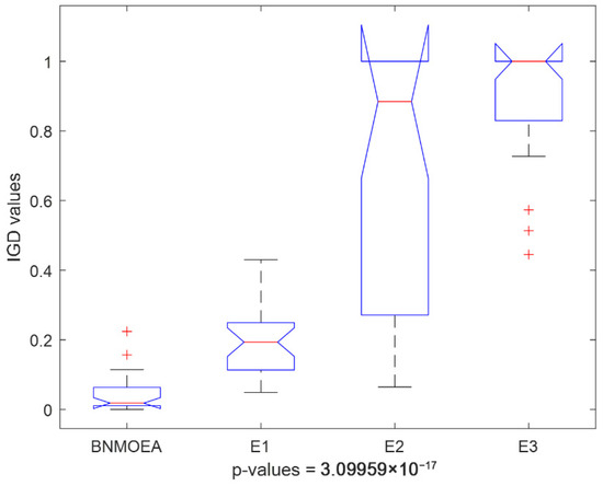
Figure 13. Kruskal–Wallis’s comparisons for the ablation experiments (IGD values).

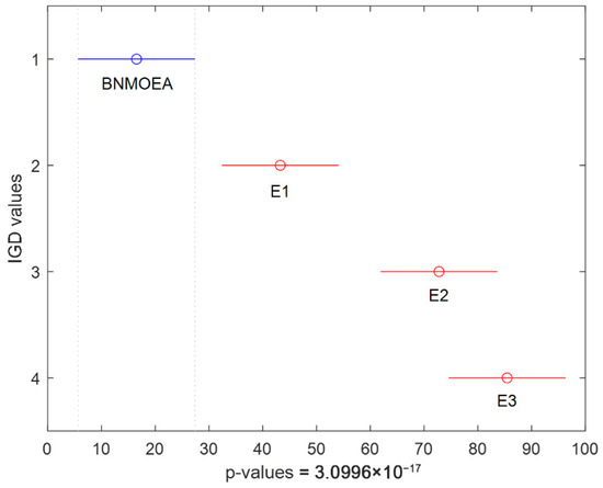
Figure 14. Friedman’s comparisons for the ablation experiments (IGD values).

To further verify the validity of the operators, the eight operators are divided into four parts, i.e., OS₁ = {SIS_cf, SEI_cf}, OS₂ = {SIS_cf, SEI_cf}, OS₃ = {SIS_cf, SEI_cf}, and OS₄ = {SIS_cf, SEI_cf}. The impact of each part on the results was verified separately as shown in Figure 15, where op-1 denotes the removal of the OS₁ operator and op-null means there are no operators. As can be seen from Figure 15a,b, all the HV values of the four-part operator operation are larger and the IGD values are smaller than those without the operator operation, so the four-part operator improves the algorithm’s performance.

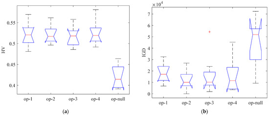
Figure 15. The results for each operator. (a) HV evaluation indicator; (b) IGD evaluation indicator.

5.5. Analysis of Comparative Algorithms

To verify the efficiency of the proposed algorithm compared with the other efficient multi-objective optimization algorithms, we chose four efficient ones, including NSGA-II [55], AGEMOEAII [56], CMOPSO [57], and BiGE [58].

Table 7, Table 8 and Table 9 illustrate the HV comparison results where the best, worst, and average results are shown in the three tables, respectively. It can be observed that (1) considering the best performance for each algorithm, the proposed BNMOEA obtained all the better values for the given 27 different-sized instances; (2) the average HV values obtained by the BNMOEA are 0.7036, 0.6318, and 0.6460 for best, worst, and average cases, which are better than the other comparison algorithms; (3) from the performance shown in the last line in the three tables, the second-best algorithm is AGEMOEAII; (4) considering the average performance, CMOPSO performs slightly better than BiGE and NSGA-II.

Table 7. Comparison of HV metric performance across algorithms (best values).

Instance_Scale	HV
	BNMOEA	AGEMOEAII	BiGE	CMOPSO	NSGAII
20 × 2 × 2 × 3	0.7036	0.6975	0.6512	0.6425	0.6787
20 × 2 × 3 × 4	0.6463	0.6183	0.5551	0.5399	0.558
20 × 2 × 4 × 5	0.6784	0.6725	0.6521	0.6379	0.6373
20 × 3 × 2 × 4	0.6692	0.6642	0.5699	0.5679	0.5739
20 × 3 × 3 × 5	0.6522	0.6568	0.5331	0.5243	0.5215
20 × 3 × 4 × 3	0.6513	0.6481	0.6262	0.6195	0.6161
20 × 4 × 2 × 5	0.6808	0.6703	0.5559	0.5348	0.6425
20 × 4 × 3 × 3	0.7094	0.6682	0.6312	0.6283	0.6345
20 × 4 × 4 × 4	0.6657	0.663	0.6424	0.6326	0.6284
60 × 2 × 2 × 3	0.6885	0.6804	0.6405	0.6485	0.6373
60 × 2 × 3 × 4	0.6466	0.6464	0.6088	0.6219	0.5827
60 × 2 × 4 × 5	0.6965	0.688	0.6434	0.659	0.6488
60 × 3 × 2 × 4	0.6852	0.6832	0.66	0.6299	0.6455
60 × 3 × 3 × 5	0.6628	0.6514	0.6319	0.6142	0.6207
60 × 3 × 4 × 3	0.6613	0.6561	0.6084	0.6054	0.6192
60 × 4 × 2 × 5	0.6463	0.6303	0.5763	0.5723	0.5747
60 × 4 × 3 × 3	0.6662	0.6531	0.616	0.6126	0.6134
60 × 4 × 4 × 4	0.6547	0.6552	0.6124	0.6026	0.613
100 × 2 × 2 × 3	0.6543	0.6561	0.6038	0.6111	0.6086
100 × 2 × 3 × 4	0.6767	0.6695	0.6269	0.6329	0.632
100 × 2 × 4 × 5	0.6611	0.6474	0.6093	0.6317	0.6087
100 × 3 × 2 × 4	0.663	0.6512	0.6113	0.6075	0.6117
100 × 3 × 3 × 5	0.653	0.6539	0.5984	0.611	0.6047
100 × 3 × 4 × 3	0.6463	0.6366	0.6015	0.5957	0.5889
100 × 4 × 2 × 5	0.6511	0.6506	0.5957	0.6086	0.5978
100 × 4 × 3 × 3	0.6555	0.646	0.6026	0.6038	0.6055
100 × 4 × 4 × 4	0.6529	0.6463	0.6273	0.6104	0.6117
Avg	0.7036	0.6975	0.6512	0.6425	0.6787

Table 8. Comparison of HV metric performance across algorithms (worst values).

Instance_Scale	HV
	BNMOEA	AGEMOEAII	BiGE	CMOPSO	NSGAII
20 × 2 × 2 × 3	0.6619	0.6499	0.4988	0.4970	0.5035
20 × 2 × 3 × 4	0.5655	0.5493	0.3684	0.3712	0.3892
20 × 2 × 4 × 5	0.6497	0.6384	0.5200	0.5086	0.5128
20 × 3 × 2 × 4	0.6097	0.5754	0.3549	0.3927	0.4113
20 × 3 × 3 × 5	0.5474	0.5403	0.3605	0.3615	0.3664
20 × 3 × 4 × 3	0.6319	0.6227	0.5143	0.5065	0.5124
20 × 4 × 2 × 5	0.6310	0.5587	0.3564	0.4474	0.3703
20 × 4 × 3 × 3	0.6456	0.6419	0.5112	0.5201	0.5407
20 × 4 × 4 × 4	0.6477	0.6393	0.5311	0.5076	0.5379
60 × 2 × 2 × 3	0.6622	0.6562	0.5566	0.5646	0.5375
60 × 2 × 3 × 4	0.6186	0.6074	0.4904	0.4952	0.4894
60 × 2 × 4 × 5	0.6717	0.6662	0.6020	0.6061	0.5907
60 × 3 × 2 × 4	0.6677	0.6576	0.5493	0.5570	0.5621
60 × 3 × 3 × 5	0.6343	0.6294	0.5185	0.5140	0.5066
60 × 3 × 4 × 3	0.6322	0.6240	0.5244	0.5363	0.5048
60 × 4 × 2 × 5	0.6165	0.6039	0.4940	0.4669	0.4686
60 × 4 × 3 × 3	0.6383	0.6283	0.5289	0.5173	0.5286
60 × 4 × 4 × 4	0.6333	0.6219	0.5279	0.5311	0.5361
100 × 2 × 2 × 3	0.6385	0.6273	0.5334	0.5371	0.5227
100 × 2 × 3 × 4	0.6560	0.6472	0.5745	0.5399	0.5717
100 × 2 × 4 × 5	0.6394	0.6318	0.5628	0.5464	0.5474
100 × 3 × 2 × 4	0.6391	0.6291	0.5123	0.5552	0.5430
100 × 3 × 3 × 5	0.6290	0.6165	0.5285	0.5305	0.5420
100 × 3 × 4 × 3	0.6171	0.6128	0.4936	0.5411	0.5133
100 × 4 × 2 × 5	0.6255	0.6178	0.5144	0.5262	0.4982
100 × 4 × 3 × 3	0.6206	0.6159	0.5199	0.5226	0.5202
100 × 4 × 4 × 4	0.6287	0.6264	0.5417	0.5490	0.5362
Avg	0.6318	0.6198	0.5033	0.5092	0.5061

Table 9. Comparison of HV metric performance across algorithms (average values).

Instance_Scale	HV
	BNMOEA	AGEMOEAII	BiGE	CMOPSO	NSGAII
20 × 2 × 2 × 3	0.6866	0.6738	0.5614	0.5630	0.5627
20 × 2 × 3 × 4	0.5827	0.5721	0.4522	0.4442	0.4486
20 × 2 × 4 × 5	0.6631	0.6546	0.5751	0.5641	0.5713
20 × 3 × 2 × 4	0.6525	0.6161	0.4642	0.4788	0.4708
20 × 3 × 3 × 5	0.5780	0.5537	0.4441	0.4452	0.4377
20 × 3 × 4 × 3	0.6399	0.6333	0.5514	0.5498	0.5506
20 × 4 × 2 × 5	0.6623	0.6218	0.4711	0.4887	0.4878
20 × 4 × 3 × 3	0.6599	0.6539	0.5727	0.5736	0.5841
20 × 4 × 4 × 4	0.6555	0.6481	0.5640	0.5541	0.5584
60 × 2 × 2 × 3	0.6747	0.6650	0.5974	0.5983	0.5968
60 × 2 × 3 × 4	0.6300	0.6220	0.5384	0.5428	0.5397
60 × 2 × 4 × 5	0.6841	0.6778	0.6219	0.6261	0.6164
60 × 3 × 2 × 4	0.6754	0.6683	0.5912	0.5945	0.5981
60 × 3 × 3 × 5	0.6495	0.6410	0.5708	0.5624	0.5634
60 × 3 × 4 × 3	0.6475	0.6397	0.5700	0.5696	0.5721
60 × 4 × 2 × 5	0.6259	0.6159	0.5327	0.5250	0.5249
60 × 4 × 3 × 3	0.6494	0.6403	0.5696	0.5682	0.5704
60 × 4 × 4 × 4	0.6404	0.6331	0.5645	0.5662	0.5747
100 × 2 × 2 × 3	0.6442	0.6395	0.5666	0.5732	0.5687
100 × 2 × 3 × 4	0.6658	0.6584	0.6022	0.5964	0.5990
100 × 2 × 4 × 5	0.6494	0.6415	0.5823	0.5897	0.5782
100 × 3 × 2 × 4	0.6493	0.6411	0.5679	0.5797	0.5745
100 × 3 × 3 × 5	0.6377	0.6275	0.5616	0.5681	0.5654
100 × 3 × 4 × 3	0.6277	0.6223	0.5554	0.5645	0.5564
100 × 4 × 2 × 5	0.6363	0.6266	0.5526	0.5606	0.5486
100 × 4 × 3 × 3	0.6339	0.6272	0.5557	0.5629	0.5568
100 × 4 × 4 × 4	0.6412	0.6363	0.5755	0.5762	0.5746
Avg	0.6460	0.6352	0.5531	0.5550	0.5537

Table 10, Table 11 and Table 12 report the IGD comparison results between the five comparison algorithms, which further verify the efficiency of the proposed BNMOEA from the best, worst, and average performance aspects.

Table 10. Comparison of IGD metric performance across algorithms (best values).

Instance_Scale	IGD
	BNMOEA	AGEMOEAII	BiGE	CMOPSO	NSGAII
20 × 2 × 2 × 3	0.0130	0.0354	0.4317	0.3924	0.1645
20 × 2 × 3 × 4	0.0001	0.0786	0.4639	0.5245	0.4250
20 × 2 × 4 × 5	0.0388	0.0782	0.4351	0.3844	0.3751
20 × 3 × 2 × 4	0.0459	0.0373	0.4755	0.4481	0.5390
20 × 3 × 3 × 5	0.0020	0.0023	0.5398	0.4919	0.2546
20 × 3 × 4 × 3	0.0155	0.0653	0.3309	0.3481	0.3720
20 × 4 × 2 × 5	0.0251	0.0571	0.2961	0.4959	0.2452
20 × 4 × 3 × 3	0.0322	0.0510	0.4906	0.4877	0.4320
20 × 4 × 4 × 4	0.0345	0.0864	0.2351	0.3625	0.4070
60 × 2 × 2 × 3	0.0160	0.0452	0.3761	0.6159	0.4611
60 × 2 × 3 × 4	0.0016	0.0018	0.4273	0.3450	0.4978
60 × 2 × 4 × 5	0.0276	0.0384	0.3533	0.3733	0.4963
60 × 3 × 2 × 4	0.0297	0.0558	0.2188	0.2648	0.3809
60 × 3 × 3 × 5	0.0565	0.0928	0.3092	0.5152	0.5003
60 × 3 × 4 × 3	0.0142	0.0499	0.5475	0.4919	0.5647
60 × 4 × 2 × 5	0.0001	0.0517	0.4194	0.4862	0.5095
60 × 4 × 3 × 3	0.0505	0.0785	0.5340	0.5123	0.5517
60 × 4 × 4 × 4	0.0379	0.0491	0.4029	0.5043	0.3905
100 × 2 × 2 × 3	0.0280	0.0267	0.4489	0.5738	0.6166
100 × 2 × 3 × 4	0.0047	0.0442	0.5130	0.5247	0.5381
100 × 2 × 4 × 5	0.0190	0.0223	0.4932	0.1898	0.4804
100 × 3 × 2 × 4	0.0243	0.0254	0.5765	0.3019	0.4021
100 × 3 × 3 × 5	0.0381	0.0272	0.5053	0.3628	0.5284
100 × 3 × 4 × 3	0.0001	0.1471	0.4093	0.3978	0.6482
100 × 4 × 2 × 5	0.0272	0.0719	0.3729	0.4022	0.4823
100 × 4 × 3 × 3	0.0090	0.0071	0.5893	0.5886	0.4820
100 × 4 × 4 × 4	0.0656	0.0898	0.2630	0.3435	0.4936
Avg	0.0243	0.0525	0.4244	0.4344	0.4533

Table 11. Comparison of IGD metric performance across algorithms (worst values).

Instance_Scale	IGD
	BNMOEA	AGEMOEAII	BiGE	CMOPSO	NSGAII
20 × 2 × 2 × 3	0.1759	0.3616	1.0000	1.0000	1.0000
20 × 2 × 3 × 4	0.3386	0.6134	1.0000	1.0000	1.0000
20 × 2 × 4 × 5	0.2769	0.5081	1.0000	1.0000	1.0000
20 × 3 × 2 × 4	0.2222	0.3363	1.0000	1.0000	1.0000
20 × 3 × 3 × 5	0.4439	0.5420	1.0000	1.0000	1.0000
20 × 3 × 4 × 3	0.2114	0.4592	1.0000	1.0000	1.0000
20 × 4 × 2 × 5	0.1243	0.3091	1.0000	1.0000	1.0000
20 × 4 × 3 × 3	0.2950	0.3945	1.0000	1.0000	1.0000
20 × 4 × 4 × 4	0.2263	0.4334	1.0000	1.0000	1.0000
60 × 2 × 2 × 3	0.2149	0.3834	1.0000	1.0000	1.0000
60 × 2 × 3 × 4	0.2928	0.3609	1.0000	1.0000	1.0000
60 × 2 × 4 × 5	0.2983	0.3664	1.0000	1.0000	1.0000
60 × 3 × 2 × 4	0.1967	0.3090	1.0000	1.0000	1.0000
60 × 3 × 3 × 5	0.2188	0.3648	1.0000	1.0000	1.0000
60 × 3 × 4 × 3	0.2326	0.2863	1.0000	1.0000	1.0000
60 × 4 × 2 × 5	0.3031	0.4003	1.0000	1.0000	1.0000
60 × 4 × 3 × 3	0.2738	0.5292	1.0000	1.0000	1.0000
60 × 4 × 4 × 4	0.2454	0.3816	1.0000	1.0000	1.0000
100 × 2 × 2 × 3	0.1913	0.3105	1.0000	1.0000	1.0000
100 × 2 × 3 × 4	0.2463	0.4595	1.0000	1.0000	1.0000
100 × 2 × 4 × 5	0.3210	0.3288	1.0000	1.0000	1.0000
100 × 3 × 2 × 4	0.1780	0.4326	1.0000	1.0000	1.0000
100 × 3 × 3 × 5	0.3072	0.4415	1.0000	1.0000	1.0000
100 × 3 × 4 × 3	0.3761	0.4185	1.0000	1.0000	1.0000
100 × 4 × 2 × 5	0.2072	0.2988	1.0000	1.0000	1.0000
100 × 4 × 3 × 3	0.2984	0.3110	1.0000	1.0000	1.0000
100 × 4 × 4 × 4	0.2666	0.2534	1.0000	1.0000	1.0000
Avg	0.2586	0.3924	1.0000	1.0000	1.0000

Table 12. Comparison of IGD metric performance across algorithms (average values).

Instance_Scale	IGD
	BNMOEA	AGEMOEAII	BiGE	CMOPSO	NSGAII
20 × 2 × 2 × 3	0.0745	0.1301	0.8642	0.8562	0.8523
20 × 2 × 3 × 4	0.2231	0.2940	0.8570	0.8455	0.8411
20 × 2 × 4 × 5	0.1320	0.1851	0.7946	0.8554	0.8127
20 × 3 × 2 × 4	0.1149	0.1637	0.8399	0.8459	0.8734
20 × 3 × 3 × 5	0.1593	0.2353	0.8558	0.8581	0.8274
20 × 3 × 4 × 3	0.1151	0.1755	0.7843	0.7924	0.8175
20 × 4 × 2 × 5	0.0709	0.1632	0.8496	0.7977	0.7973
20 × 4 × 3 × 3	0.1333	0.1952	0.9161	0.8692	0.8136
20 × 4 × 4 × 4	0.1211	0.1699	0.7734	0.8507	0.8424
60 × 2 × 2 × 3	0.1004	0.1826	0.8645	0.8368	0.8749
60 × 2 × 3 × 4	0.1728	0.2296	0.8907	0.8512	0.8451
60 × 2 × 4 × 5	0.1260	0.1738	0.8150	0.8093	0.8818
60 × 3 × 2 × 4	0.1291	0.1668	0.8947	0.8392	0.8280
60 × 3 × 3 × 5	0.1232	0.1728	0.8000	0.8638	0.8648
60 × 3 × 4 × 3	0.0993	0.1761	0.8415	0.8743	0.8445
60 × 4 × 2 × 5	0.1455	0.2115	0.8481	0.8638	0.8701
60 × 4 × 3 × 3	0.1398	0.2167	0.8589	0.8529	0.8684
60 × 4 × 4 × 4	0.1220	0.1785	0.8321	0.8736	0.8291
100 × 2 × 2 × 3	0.0981	0.1438	0.8641	0.8337	0.8828
100 × 2 × 3 × 4	0.1064	0.2117	0.8412	0.8607	0.8739
100 × 2 × 4 × 5	0.1254	0.2178	0.8666	0.7405	0.9047
100 × 3 × 2 × 4	0.0802	0.1647	0.8841	0.8043	0.8777
100 × 3 × 3 × 5	0.1412	0.2171	0.8971	0.7679	0.8374
100 × 3 × 4 × 3	0.2127	0.2847	0.8467	0.7995	0.8775
100 × 4 × 2 × 5	0.1109	0.1653	0.8375	0.7845	0.8739
100 × 4 × 3 × 3	0.1253	0.1691	0.8895	0.8221	0.8362
100 × 4 × 4 × 4	0.1456	0.1733	0.8159	0.8183	0.8472
Avg	0.1277	0.1914	0.8490	0.8321	0.8517

Figure 16 illustrates the Kruskal–Wallis comparisons for HV values among the five comparison algorithms, while Figure 17 reports the trend of HV values with increasing instances scale. The two figures verify the efficiency of the proposed algorithm considering the HV indicator. Figure 18 illustrates the Kruskal–Wallis comparisons for the BNMOEA, AGEMOEAII, BiGE, CMOPSO, and NSGAII considering the IGD values, while the trend of IGD values with increasing scale was reported in Figure 19. The two figures also verify the effectiveness of the proposed algorithm considering the IGD indicator.

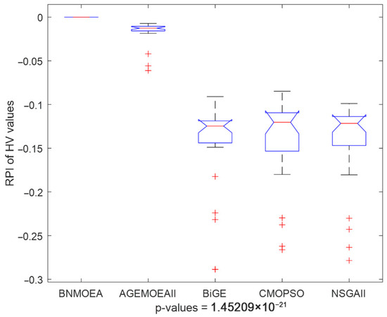
Figure 16. Kruskal–Wallis’s comparisons for BNMOEA, AGEMOEAII, BiGE, CMOPSO, and NSGAII (HV values).

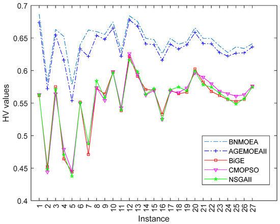
Figure 17. Change trend of HV values with increasing instances scale.

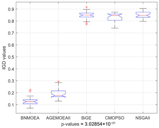
Figure 18. Kruskal–Wallis’s comparisons for BNMOEA, AGEMOEAII, BiGE, CMOPSO, and NSGAII (IGD values).

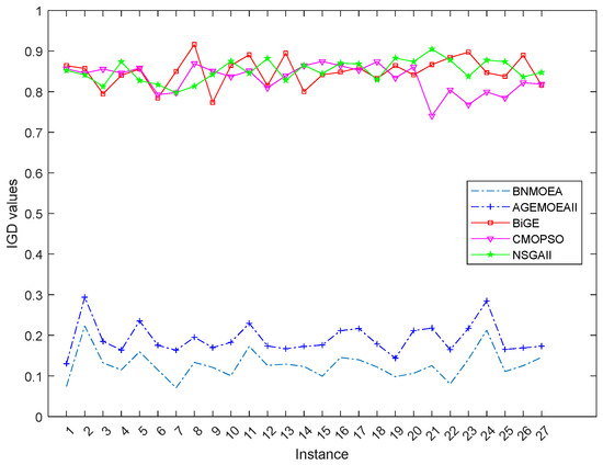
Figure 19. Change trend of IGD values with increasing instances scale.

In addition, we have tested the above comparison algorithms using the Empirical Achievement Function (EAF) [65]. In the EAF, the color indicates the difference in the probability of this algorithm dominating the corresponding solution compared with another algorithm. The higher the difference, the darker the color, and the higher the probability that the result obtained here will dominate the solution compared with another algorithm. In short, the darker the color and the larger the area, the better the algorithm. The following conclusions can be obtained from Figure 20: (1) The shaded portion of the BNMOEA is larger than the other comparison algorithms, which proves that the BNMOEA has a better performance. (2) The BNMOEA also outperforms the other four comparative algorithms under different scheduling environments. Therefore, the EAF demonstrates that the BNMOEA has an excellent performance.

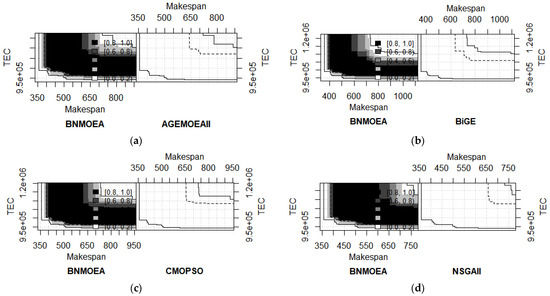
Figure 20. EAF differences between BNMOEA and other algorithms for instance 20 × 2 × 2 × 3. (a) The differences between BNMOEA and AGEMOEAII; (b) the differences between BNMOEA and BiGE; (c) the differences between BNMOEA and CMOPSO; (d) the differences between BNMOEA and NSGAII.

6. Conclusions

A more practical problem with resource constraints and machine breakdown in the DHFSP was considered and solved using a BNMOEA. The BNMOEA improves the searching capability, which includes a hybrid initialization method and local reinforcement-based critical factories. The effect of hybrid initialization methods and local search on the BNMOEA is tested through extensive experiments. The BNMOEA was also compared with four comparison algorithms. The experimental results show that the BNMOEA is a great solution to address DRCHFSP-MB.

The main limitations of the current study are as follows: (1) because there are few studies considering both limited resource and machine breakdown constraints simultaneously in the DHFSP, the benchmarks should be generated in a more reasonable manner; (2) the algorithm embeds the initialization heuristic and global and local search operators, but how to design problem-specific components with a more efficient performance is still a challenging task.

Therefore, future work can consider the following aspects: (1) apply the proposed multi-objective optimization to solve the DHFSP with limited resources and machine breakdown constraints in distributed heterogeneous factories; (2) design benchmarks for the considered problem and provide the Pareto front results; (3) design more problem-specific and efficient strategies to enhance both the global and local search capabilities; (4) consider other realistic constraints and objectives, such as random job arrival, random order cancelation, and economic objectives.

References

- Li, J.; Li, J.; Gao, K.; Duan, P. A hybrid graph-based imitation learning method for a realistic distributed hybrid flow shop with family setup time. IEEE Trans. Syst. Man Cybern. Syst. 2024, 54, 7291–7304. [Google Scholar] [CrossRef]
- Song, H.; Li, J.; Du, Z.; Yu, X.; Xu, Y.; Zheng, Z.; Li, J. A Q-learning driven multi-objective evolutionary algorithm for worker fatigue dual-resource-constrained distributed hybrid flow shop. Comput. Oper. Res. 2025, 175, 106919. [Google Scholar] [CrossRef]
- Luo, H.; Du, B.; Huang, G.Q.; Chen, H.; Li, X. Hybrid flow shop scheduling considering machine electricity consumption cost. Int. J. Prod. Econ. 2013, 146, 423–439. [Google Scholar] [CrossRef]
- Wei, Z.; Liao, W.; Zhang, L. Hybrid energy-efficient scheduling measures for flexible job-shop problem with variable machining speeds. Expert Syst. Appl. 2022, 197, 116785. [Google Scholar] [CrossRef]
- Liu, Q.; Pan, Q.K.; Gao, L.; Li, X. Multi-objective flexible job shop scheduling problem considering machine switching off-on operation. Procedia Manuf. 2019, 39, 1167–1176. [Google Scholar] [CrossRef]
- Abtahi, Z.; Sahraeian, R. Robust and Stable Flow Shop Scheduling Problem Under Uncertain Processing Times and Machines Disruption. Int. J. Eng. Trans. A Basics 2021, 34, 935–947. [Google Scholar]
- Hosseini, S.M.H.; Sana, S.S.; Rostami, M. Assembly flow shop scheduling problem considering machine eligibility restrictions and auxiliary resource constraints. Int. J. Syst. Sci. Oper. Logist. 2022, 9, 512–528. [Google Scholar] [CrossRef]
- Ying, K.C.; Lin, S.W. Minimizing makespan for the distributed hybrid flowshop scheduling problem with multiprocessor tasks. Expert Syst. Appl. 2018, 92, 132–141. [Google Scholar] [CrossRef]
- Li, Y.; Li, F.; Pan, Q.K.; Gao, L.; Tasgetiren, M.F. An artificial bee colony algorithm for the distributed hybrid flowshop scheduling problem. Procedia Manuf. 2019, 39, 1158–1166. [Google Scholar] [CrossRef]
- Cai, J.; Zhou, R.; Lei, D. Dynamic shuffled frog-leaping algorithm for distributed hybrid flow shop scheduling with multiprocessor tasks. Eng. Appl. Artif. Intell. 2020, 90, 103540. [Google Scholar] [CrossRef]
- Du, Y.; Li, J.; Chen, X.; Duan, P.; Pan, Q. Knowledge-Based Reinforcement Learning and Estimation of Distribution Algorithm for Flexible Job Shop Scheduling Problem. IEEE Trans. Emerg. Top. Comput. Intell. 2022, 7, 1036–1050. [Google Scholar] [CrossRef]
- Wang, S.; Wu, R.; Chu, F.; Yu, J. Variable neighborhood search-based methods for integrated hybrid flow shop scheduling with distribution. Soft Comput. 2020, 24, 8917–8936. [Google Scholar] [CrossRef]
- Zheng, J.; Wang, L.; Wang, J. A cooperative coevolution algorithm for multi-objective fuzzy distributed hybrid flow shop. Knowl.-Based Syst. 2020, 194, 105536. [Google Scholar] [CrossRef]
- Shao, W.; Shao, Z.; Pi, D. Modeling and multi-neighborhood iterated greedy algorithm for distributed hybrid flow shop scheduling problem. Knowl.-Based Syst. 2020, 194, 105527. [Google Scholar] [CrossRef]
- Wang, J.; Wang, L. A Bi-Population Cooperative Memetic Algorithm for Distributed Hybrid Flow-Shop Scheduling. IEEE Trans. Emerg. Top. Comput. Intell. 2021, 5, 947–961. [Google Scholar] [CrossRef]
- Shao, W.; Shao, Z.; Pi, D. Multi-objective evolutionary algorithm based on multiple neighborhoods local search for multi-objective distributed hybrid flow shop scheduling problem. Expert Syst. Appl. 2021, 183, 115453. [Google Scholar] [CrossRef]
- Li, Q.; Li, J.; Zhang, X.; Zhang, B. A wale optimization algorithm for distributed flow shop with batch delivery. Soft Comput. 2021, 25, 13181–13194. [Google Scholar] [CrossRef]
- Wang, J.; Wang, L. A Cooperative Memetic Algorithm with Learning-Based Agent for Energy-Aware Distributed Hybrid Flow-Shop Scheduling. IEEE Trans. Evol. Comput. 2022, 26, 461–475. [Google Scholar] [CrossRef]
- Lu, C.; Liu, Q.; Zhang, B.; Yin, L. A Pareto-based hybrid iterated greedy algorithm for energy-efficient scheduling of distributed hybrid flowshop. Expert Syst. Appl. 2022, 204, 117555. [Google Scholar] [CrossRef]
- Shao, W.; Shao, Z.; Pi, D. A network memetic algorithm for energy and labor-aware distributed heterogeneous hybrid flow shop scheduling problem. Swarm Evol. Comput. 2022, 75, 101190. [Google Scholar] [CrossRef]
- Meng, L.; Gao, K.; Ren, Y.; Zhang, B.; Sang, H.; Zhang, C. Novel MILP and CP models for distributed hybrid flowshop scheduling problem with sequence-dependent setup times. Swarm Evol. Comput. 2022, 71, 101058. [Google Scholar] [CrossRef]
- Lei, D.; Su, B. A multi-class teaching–learning-based optimization for multi-objective distributed hybrid flow shop scheduling. Knowl.-Based Syst. 2023, 263, 110252. [Google Scholar] [CrossRef]
- Gholami, H.; Sun, H. Toward automated algorithm configuration for distributed hybrid flow shop scheduling with multiprocessor tasks. Knowl.-Based Syst. 2023, 264, 110309. [Google Scholar] [CrossRef]
- Gholami, M.; Zandieh, M.; Alem-Tabriz, A. Scheduling hybrid flow shop with sequence-dependent setup times and machines with random breakdowns. Int. J. Adv. Manuf. Technol. 2008, 42, 189–201. [Google Scholar] [CrossRef]
- Zandieh, M.; Gholami, M. An immune algorithm for scheduling a hybrid flow shop with sequence-dependent setup times and machines with random breakdowns. Int. J. Prod. Res. 2009, 47, 6999–7027. [Google Scholar] [CrossRef]
- Safari, E.; Sadjadi, S.J. A hybrid method for flowshops scheduling with condition-based maintenance constraint and machines breakdown. Expert Syst. Appl. 2011, 38, 2020–2029. [Google Scholar] [CrossRef]
- Wang, K.; Choi, S.H. A decomposition-based approach to flexible flow shop scheduling under machine breakdown. Int. J. Prod. Res. 2011, 50, 215–234. [Google Scholar] [CrossRef]
- Mirabi, M.; Ghomi, S.M.T.F.; Jolai, F. A two-stage hybrid flowshop scheduling problem in machine breakdown condition. J. Intell. Manuf. 2011, 24, 193–199. [Google Scholar] [CrossRef]
- Wang, K.; Huang, Y.; Qin, H. A fuzzy logic-based hybrid estimation of distribution algorithm for distributed permutation flowshop scheduling problems under machine breakdown. J. Oper. Res. Soc. 2017, 67, 68–82. [Google Scholar] [CrossRef]
- Adressi, A.; Tasouji Hassanpour, S.; Azizi, V. Solving group scheduling problem in no-wait flexible flowshop with random machine breakdown. Decis. Sci. Lett. 2016, 5, 157–168. [Google Scholar] [CrossRef]
- Fazayeli, M.; Aleagha, M.R.; Bashirzadeh, R.; Shafaei, R. A hybrid meta-heuristic algorithm for flowshop robust scheduling under machine breakdown uncertainty. Int. J. Comput. Integr. Manuf. 2016, 29, 709–719. [Google Scholar] [CrossRef]
- Seidgar, H.; Rad, S.T.; Shafaei, R. Scheduling of assembly flow shop problem and machines with random breakdowns. Int. J. Oper. Res. 2017, 29, 273–293. [Google Scholar] [CrossRef]
- Han, Y.; Gong, D.; Jin, Y.; Pan, Q. Evolutionary Multiobjective Blocking Lot-Streaming Flow Shop Scheduling with Machine Breakdowns. IEEE Trans. Cybern. 2019, 49, 184–197. [Google Scholar] [CrossRef] [PubMed]
- Tadayonirad, S.; Seidgar, H.; Fazlollahtabar, H.; Shafaei, R. Robust scheduling in two-stage assembly flow shop problem with random machine breakdowns: Integrated meta-heuristic algorithms and simulation approach. Assem. Autom. 2019, 39, 944–962. [Google Scholar] [CrossRef]
- Marichelvam, M.K.; Geetha, M. A hybrid algorithm to solve the stochastic flow shop scheduling problems with machine break down. Int. J. Enterp. Netw. Manag. 2019, 10, 162–175. [Google Scholar] [CrossRef]
- Seidgar, H.; Fazlollahtabar, H.; Zandieh, M. Scheduling two-stage assembly flow shop with random machines breakdowns: Integrated new self-adapted differential evolutionary and simulation approach. Soft Comput. 2020, 24, 8377–8401. [Google Scholar] [CrossRef]
- Branda, A.; Castellano, D.; Guizzi, G.; Popolo, V. Metaheuristics for the flow shop scheduling problem with maintenance activities integrated. Comput. Ind. Eng. 2021, 151, 106989. [Google Scholar] [CrossRef]
- Li, J.; Li, R.; Li, J.; Yu, X.; Xu, Y. A multi-dimensional co-evolutionary algorithm for multi-objective resource-constrained flexible flowshop with robotic transportation. Appl. Soft Comput. 2025, 170, 112689. [Google Scholar] [CrossRef]
- Leu, S.S.; Hwang, S.T. GA-based resource-constrained flow-shop scheduling model for mixed precast production. Autom. Constr. 2002, 11, 439–452. [Google Scholar] [CrossRef]
- Jarboui, B.; Damak, N.; Siarry, P.; Rebai, A. A combinatorial particle swarm optimization for solving multi-mode resource-constrained project scheduling problems. Appl. Math. Comput. 2008, 195, 299–308. [Google Scholar] [CrossRef]
- Behnamian, J.; Fatemi Ghomi, S.M.T. Hybrid flowshop scheduling with machine and resource-dependent processing times. Appl. Math. Model. 2011, 35, 1107–1123. [Google Scholar] [CrossRef]
- Rajkumar, M.; Asokan, P.; Anilkumar, N.; Page, T. A GRASP algorithm for flexible job-shop scheduling problem with limited resource constraints. Int. J. Prod. Res. 2011, 49, 2409–2423. [Google Scholar] [CrossRef]
- Cheng, T.C.E.; Lin, B.M.T.; Huang, H.L. Resource-constrained flowshop scheduling with separate resource recycling operations. Comput. Oper. Res. 2012, 39, 1206–1212. [Google Scholar] [CrossRef]
- Lin, D.; Lee, C.K.; Ho, W. Multi-level genetic algorithm for the resource-constrained re-entrant scheduling problem in the flow shop. Eng. Appl. Artif. Intell. 2013, 26, 1282–1290. [Google Scholar] [CrossRef]
- Bożejko, W.; Hejducki, Z.; Uchroński, M.; Wodecki, M. Solving Resource-Constrained Construction Scheduling Problems with Overlaps by Metaheuristic. J. Civ. Eng. Manag. 2014, 20, 649–659. [Google Scholar] [CrossRef]
- Laribi, I.; Yalaoui, F.; Belkaid, F.; Sari, Z. Heuristics for solving flow shop scheduling problem under resources constraints. IFAC-Pap. 2016, 49, 1478–1483. [Google Scholar] [CrossRef]
- Rahman, H.; Chakrabortty, R.; Ryan, M. Memetic algorithm for solving resource constrained project scheduling problems. Autom. Constr. 2020, 111, 103052. [Google Scholar] [CrossRef]
- Costa, A.; Fernandez-Viagas, V.; Framinan, J. Solving the hybrid flow shop scheduling problem with limited human resource constraint. Comput. Ind. Eng. 2020, 146, 106545. [Google Scholar] [CrossRef]
- Boufellouh, R.; Belkaid, F. Bi-objective optimization algorithms for joint production and maintenance scheduling under a global resource constraint: Application to the permutation flow shop problem. Comput. Oper. Res. 2020, 122, 104943. [Google Scholar] [CrossRef]
- Chen, X.; Li, J.; Wang, Z.; Chen, Q.; Gao, K.; Pan, Q. Optimizing dynamic flexible job shop scheduling using an evolutionary multi-task optimization framework and genetic programming. IEEE Trans. Evol. Comput. 2025, 29, 1502–1516. [Google Scholar] [CrossRef]
- Han, W.; Deng, Q.; Gong, G.; Zhang, L.; Luo, Q. Multi-objective evolutionary algorithms with heuristic decoding for hybrid flow shop scheduling problem with worker constraint. Expert Syst. Appl. 2021, 168, 114282. [Google Scholar] [CrossRef]
- Hasani, A.; Hosseini, S.M.H. Auxiliary resource planning in a flexible flow shop scheduling problem considering stage skipping. Comput. Oper. Res. 2022, 138, 105625. [Google Scholar] [CrossRef]
- Zuo, Y.; Zhao, F.; Yu, Y. Two-stage learning scatter search algorithm for the distributed hybrid flow shop scheduling problem with machine breakdown. Expert Syst. Appl. 2025, 259, 125344. [Google Scholar] [CrossRef]
- Tian, Y.; Cheng, R.; Zhang, X.; Jin, Y. PlatEMO: A MATLAB platform for evolutionary multi-objective optimization [educational forum]. IEEE Comput. Intell. Mag. 2017, 12, 73–87. [Google Scholar] [CrossRef]
- Deb, K.; Pratap, A.; Agarwal, S.; Meyarivan, T. A fast and elitist multiobjective genetic algorithm: NSGA-II. IEEE Trans. Evol. Comput. 2002, 6, 182–197. [Google Scholar] [CrossRef]
- Panichella, A. An improved Pareto front modeling algorithm for large-scale many-objective optimization. In Proceedings of the Genetic and Evolutionary Computation Conference, Boston, MA, USA, 9–13 July 2022; pp. 565–573. [Google Scholar]
- Zhang, X.; Zheng, X.; Cheng, R.; Qiu, J.; Jin, Y. A competitive mechanism based multi-objective particle swarm optimizer with fast convergence. Inf. Sci. 2018, 427, 63–76. [Google Scholar] [CrossRef]
- Li, M.; Yang, S.; Liu, X. Bi-goal evolution for many-objective optimization problems. Artif. Intell. 2015, 228, 45–65. [Google Scholar] [CrossRef]
- Du, Y.; Li, J.; Li, C.; Duan, P. A Reinforcement Learning Approach for Flexible Job Shop Scheduling Problem with Crane Transportation and Setup Times. IEEE Trans. Neural Netw. Learn. Syst. 2024, 35, 5695–5709. [Google Scholar] [CrossRef]
- Du, Z.S.; Li, J.Q.; Song, H.N.; Gao, K.Z.; Xu, Y.; Li, J.K.; Zheng, Z.X. Solving the permutation flow shop scheduling problem with sequence-dependent setup time via iterative greedy algorithm and imitation learning. Math. Comput. Simul. 2025, 234, 169–193. [Google Scholar] [CrossRef]
- Duan, J.; Liu, F.; Zhang, Q.; Qin, J.; Zhou, Y. Genetic programming hyper-heuristic-based solution for dynamic energy-efficient scheduling of hybrid flow shop scheduling with machine breakdowns and random job arrivals. Expert Syst. Appl. 2024, 254, 124375. [Google Scholar] [CrossRef]
- Duan, J.; Liu, F.; Zhang, Q.; Qin, J. Tri-objective lot-streaming scheduling optimization for hybrid flow shops with uncertainties in machine breakdowns and job arrivals using an enhanced genetic programming hyper-heuristic. Comput. Oper. Res. 2024, 172, 106817. [Google Scholar] [CrossRef]
- Li, J.; Han, Y.; Gao, K.; Xiao, X.; Duan, P. Bi-population balancing multi-objective algorithm for fuzzy flexible job shop with energy and transportation. IEEE Trans. Autom. Sci. Eng. 2024, 21, 4686–4702. [Google Scholar] [CrossRef]
- Li, J.; Li, J.; Xu, Y. HGNP: A PCA-based heterogeneous graph neural network for a family distributed flexible job shop. Comput. Ind. Eng. 2025, 200, 110855. [Google Scholar] [CrossRef]
- López-Ibáñez, M.; Paquete, L.; Stützle, T. Exploratory analysis of stochastic local search algorithms in biobjective optimization. In Experimental Methods for the Analysis of Optimization Algorithms; Springer: Berlin/Heidelberg, Germany, 2010. [Google Scholar]
- Wang, Y.; Li, J.; Yang, Z.; Zhang, H.; Li, J.; Duan, P.; Du, Y.; Ning, C. An adaptive collaborative optimization algorithm for hybrid flow shop with group setup times and consistent sublots. Appl. Math. Model. 2025, 150, 116354. [Google Scholar] [CrossRef]
- Wang, Z.; Li, J.; Chen, X.; Duan, P.; Li, J. Uncertain Interruptibility Multiobjective Flexible Job Shop via Deep Reinforcement Learning Based on Heterogeneous Graph Self-Attention. IEEE Trans. Neural Netw. Learn. Syst. 2025, 36, 18598–18612. [Google Scholar] [CrossRef]
- Candan, G.; Yazgan, H. Genetic algorithm parameter optimisation using Taguchi method for a flexible manufacturing system scheduling problem. Int. J. Prod. Res. 2015, 53, 897–915. [Google Scholar] [CrossRef]
Disclaimer/Publisher’s Note: The statements, opinions and data contained in all publications are solely those of the individual author(s) and contributor(s) and not of MDPI and/or the editor(s). MDPI and/or the editor(s) disclaim responsibility for any injury to people or property resulting from any ideas, methods, instructions or products referred to in the content. |
© 2025 by the authors. Licensee MDPI, Basel, Switzerland. This article is an open access article distributed under the terms and conditions of the Creative Commons Attribution (CC BY) license (https://creativecommons.org/licenses/by/4.0/).