Development, Implementation and Experimental Assessment of Path-Following Controllers on a 1:5 Scale Vehicle Testbed

Abstract

The development of control strategies for autonomous vehicles requires a reliable and cost-effective validation approach. In this context, testbeds enabling repeatable experiments under controlled conditions are gaining relevance. Scaled vehicles have proven to be a valuable alternative to full-scale or simulation-based testing, enabling experimental validation while reducing costs and risks. This work presents a 1:5 scale modular vehicle platform, derived from a commercial Radio-Controlled (RC) vehicle and adapted as experimental testbed for control strategy validation and vehicle dynamics studies. The vehicle features an electric powertrain, operated through a Speedgoat Baseline Real-Time Target Machine (SBRTM). The hardware architecture includes a high-performance Inertial Measurement Unit (IMU) with embedded Global Navigation Satellite System (GNSS). An Extended Kalman Filter (EKF) is implemented to enhance positioning accuracy by fusing inertial and GNSS data, providing reliable estimates of the vehicle position, velocity, and orientation. Two path-following algorithms, i.e., Stanley Controller (SC) and the Linear Quadratic Regulator (LQR), are designed and integrated. Outdoor experimental tests enable the evaluation of tracking accuracy and robustness. The results demonstrate that the proposed scaled testbed constitutes a reliable and flexible platform for benchmarking autonomous vehicle controllers and enabling experimental testing.

1. Introduction

The growing interest in automated driving necessitates robust and systematic validation methodologies to design, test, and assess Advanced Driver Assistance Systems (ADAS) [1,2].

As human error remains the predominant cause of accidents [3], safety-oriented technologies have been progressively introduced to mitigate critical situations. Thanks to the increased computational power of current processors, modern safety systems are able to guarantee prompt response in hazardous conditions [4]. New systems, such as Adaptive Cruise Control [5,6], Blind Spot Detection [7], Automated Lane Change [8], and Driver Lane Change Intention Prediction [9], have also been developed, thereby fostering the development of driverless vehicles [10]. This evolution requires comprehensive testing infrastructures tailored to the specific scenario under investigation [11,12]. In the literature, three main testing approaches are reported as follows [13]: full-scale vehicle on-road/on-track testing [14], computer simulations [12,15], and scaled vehicle experimental testing [16].

• The first scenario involves full-scale on-road testing, which is considered the most effective and precise approach, as it can capture the whole vehicle interactions in real-world conditions [13]. However, this methodology requires dedicated test facilities, high-performance sensors [17], and compliance with regulatory and logistical constraints. While it provides high-fidelity data, this approach suffers from limited replicability, since recreating identical scenarios is challenging due to environmental variability. Moreover, on-road tests may expose occupants and pedestrians to potential safety risks [18].
• The second approach, i.e., computer simulations, enables replicability and can be tailored to parametric investigations of road characteristics, e.g., intersection angle, curvature, and lane width [19]. Nevertheless, this methodology inherently depends on the accuracy level of the employed models, which strongly influences the reliability of the obtained results [20]. Among the simulation environments, AIMSUN [21], Vissim [22], and Silo [23] are used the most for small and medium-scale traffic flow analysis. The open-source SUMO [24] is particularly suited for large-scale traffic simulations and for integration with external control and communication frameworks. Gazebo [25] is effective for sensor and actuator simulation. CARLA [26,27] provides realistic 3D environments, dynamic weather conditions, and high-fidelity sensor models. In contrast, CarSim [28,29] offers highly accurate vehicle dynamics models and is often used together with MATLAB/Simulink R2024a [30] for controller development and hardware-in-the-loop testing. Finally, the Cellular Automata approaches [31] are employed when simplified yet computationally efficient representations of traffic are sufficient.
• To mitigate the cost, safety, and model-dependence limitations associated with full-scale and simulation-based testing, scaled vehicles have gained increasing attention in recent years [32], although their usage dates back to the 1930s for studying trailer sway, turning radius, and automobile accident reconstruction [33]. These platforms offer a cost-effective alternative to full-scale testing; they are easy to operate without requiring specialized training, involve limited maintenance, and require only small test facilities. Moreover, they are typically characterized by a high modularity level in terms of embedded sensors and components. A comprehensive overview of recent developments, applications, and technological trends in small-scale self-driving vehicles is provided in [20].

These platforms are generally derived from Radio-Controlled (RC) cars [18,32,34], which undergo hardware modification, and are driven by electric powertrains, allowing smoother and more precise control, since they are less affected by vibration issues [2] and suitable for indoor testing.

The sensor setup of scaled vehicles generally includes a three-axis Inertial Measurement Unit (IMU) providing acceleration signals required by control algorithms. In [34], these signals are provided as inputs to a particle filter to enhance real-time vehicle localization. Global Positioning Systems (GPS)/Global Navigation Satellite System (GNSS) are typically adopted for trajectory reconstruction [35,36], while LiDAR sensors are adopted for environmental identification and obstacle detection [37]. Cameras are primarily employed for lane keeping and traffic sign recognition [38]. Data acquisition, decision-making, and control tasks are handled by embedded computing units such as Raspberry Pi and NVIDIA Jetson.

Despite their compact size, these platforms can achieve speeds and accelerations comparable to full-scale vehicles, making them reliable tools for investigating vehicle dynamics and testing complex control algorithms under challenging conditions, including drifting and rally like maneuvers [34,39].

As shown in [20], the most common scales for these kinds of testbeds, in order of popularity, are $1:5$, $1:10$, and $1:43$. Larger scales, such as $1:5$, are particularly suitable for vehicle dynamics studies, as they better reproduce the behavior of full-scale passenger cars and allow the integration of standard-sized sensors. Nevertheless, they require more powerful motors and larger test areas. Conversely, smaller scales such as $1:10$ or $1:43$ are cost-effective, since they rely on smaller actuators and require smaller experimental facilities. These smaller platforms are often adopted for platooning studies, whereas larger ones are preferred for more detailed investigations of vehicle dynamics [40].

Among the most recent developments, an open-source platform for high-speed off-road driving research is presented in [32]. Built on a similar concept, Baumann et al. [41] introduce the ForzaETH Race Stack, a $1:10$ scale platform, based on off-the-shelf components. Finally, other $1:10$ scale platforms featuring advanced sensor modules for key control signals are proposed in [18,37], providing low-cost self-driving vehicle testbeds for indoor experimentation. These platforms differ primarily in their development approach, ranging from fully custom designs, in the former, to adaptations of commercial RC vehicles, in the latter.

From a control perspective, scaled vehicles have proven to be a valuable tool for validating advanced control methodologies, as stated by Ribeiro et al. [16]. Švec et al. [42] evaluate Koopman operator-based models on reduced-scale platforms, confirming their potential for capturing nonlinear vehicle dynamics. Cataffo et al. [43] develop a Nonlinear Model Predictive Control (NMPC) strategy and deploy it on a $1:10$ scale platform to minimize lap times in Autonomous Vehicles racing scenarios. Bohn et al. [44] present a dedicated custom-scale platform, the ZeloS, equipped with advanced perception and communication sensors, specifically designed to support the development and validation of autonomous driving algorithms. Similarly, Natvig et al. [23] employ scaled vehicles to test machine learning-based approaches, such as reinforcement learning, taking advantage of their ability to perform fast and repeatable experiments with lower costs and risks. In addition, scaled vehicles are also shown to be effective in estimating key vehicle parameters, such as cornering stiffness and yaw moment of inertia, through identification methods based on the vehicle’s lateral dynamic [16]. Other studies focus on advanced control strategies for drifting; Domberg et al. [4] employed deep neural network-based controllers, Zhou et al. [45] develop a model predictive control framework, Park and Kang [46] propose a two-level controller, combining path-tracking and steady-state drift control. These last three approaches have been successfully validated on $1:10$ scale RC cars. Additional applications include road profile estimation, as demonstrated by Tudon–Martinez et al. [47], or the development of LiDAR-equipped platforms for cooperative driving and platooning experiments, as shown by Miller [48].

Very few studies explore the implementation of the Stanley Controller (SC) and the Linear Quadratic Regulator (LQR) on scaled vehicles; the existing works typically concentrate either on vehicle-dynamics analysis or on the validation of path-following strategies performed in controlled or semi-controlled environments [16,20]. These proving grounds inherently avoid the challenges introduced by realistic outdoor operation, in which terrain irregularities and environmental disturbances significantly affect test execution and repeatability. In addition, GNSS measurements are rarely employed on scaled platforms, as most experimental setups rely on optical tracking systems, which require lane markings or structured reference lines for localization. To the best of the authors’ knowledge, no prior work has experimentally compared multiple trajectory-tracking controllers in uncontrolled outdoor conditions using a modular scaled vehicle platform.

To address this gap, the present study introduces a $1:5$ scale platform, originally customized and validated in open-loop maneuvers [2], which is further upgraded with enhanced hardware to support fully autonomous repeatable, infrastructure-free, outdoor operation through a sensor-fusion approach exploiting GNSS-aided state estimation. This configuration enables experimental conditions that are not typically addressed in existing scaled-vehicle studies. The main features of the platform are as follows:

• Complete hardware modularity and software reconfigurability;
• Realistic double-wishbone suspension;
• Electrified powertrain providing smooth torque delivery and precise low-speed control, suitable for both indoor and outdoor experiments;
• A dedicated control strategy for trajectory tracking;
• Use of low-cost commercial sensors supported by accurate sensor-fusion estimation algorithms.

The enhanced platform includes an IMU with embedded GNSS able to communicate via CAN protocol. Regarding the software, an Extended Kalman Filter (EKF) is implemented to enhance position estimation by fusing IMU and GNSS data. Two alternative path-following control strategies, i.e., the SC and the LQR, have been developed and integrated into the real-time architecture, exploiting more accurate estimation provided by the EKF. These improvements collectively enhance closed-loop maneuver testing [2].

The paper is organized as follows:

• Section 2 provides a detailed overview of the testbed, describing the hardware and its main features;
• Section 3 presents the development and the implementation of the path-following control algorithms;
• Section 4 illustrates test procedures, detailing maneuvers and facilities;
• Section 5 summarizes the main findings of the activity;
• Section 6 assesses the overall effectiveness of the proposed research and outlines possible future developments.

2. Vehicle Overview

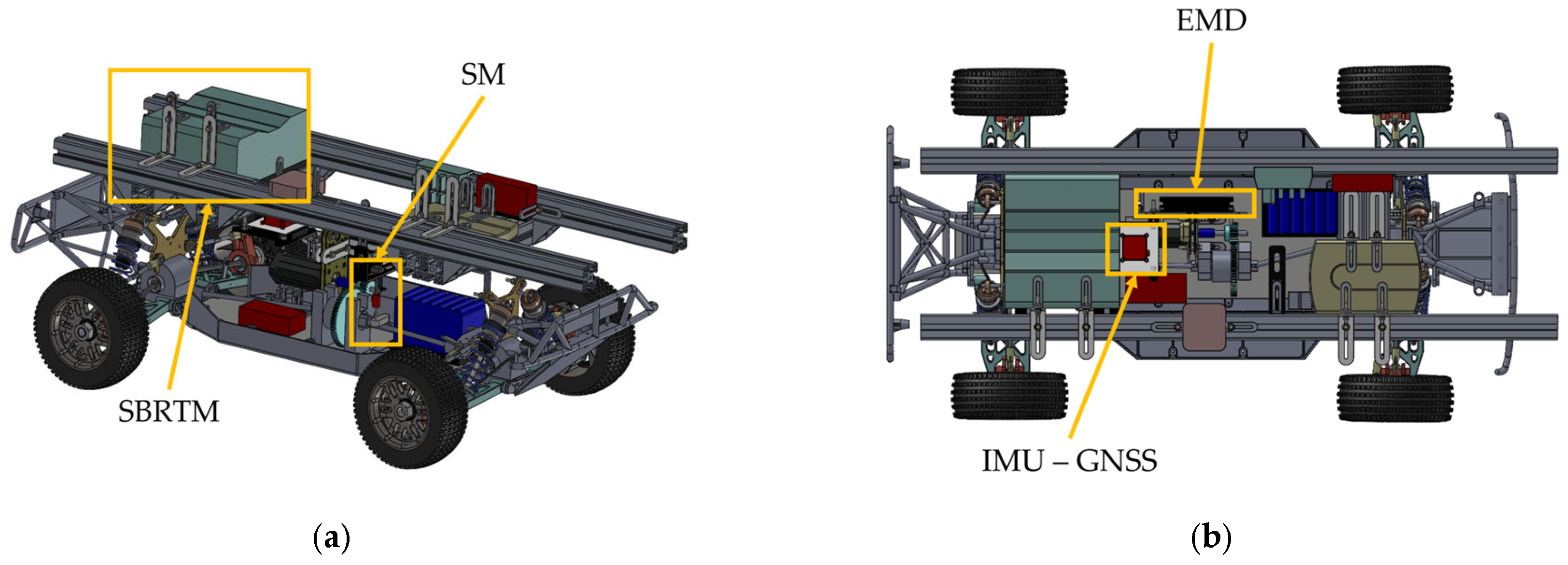
The experimental platform employed in this study, shown in Figure 1, is a $1:5$ scale modular testbed, whose preliminary version was presented in [2] and which has been upgraded to enable path-tracking capabilities. The chassis is based on a commercial radio-controlled vehicle equipped with a $32$ cc two-stroke Internal Combustion Engine (ICE) and a four-wheel-drive fixed-gear transmission, comprising three open differentials: one inter-axle and one inter-wheel differential per axle.

Figure 1. Details of the main hardware on the 1:5 scale vehicle: isometric view (a) and top view (b).

The suspension adopts an independent double-arm geometry at all four corners, each equipped with springs, dampers, and anti-roll bars. Camber and toe angles are adjustable at the front and at the rear within the range $\pm 5°$. The chassis geometry is characterized by the wheelbase $l=0.61$ m, track width $t=0.45$ m, and wheel radius $r_w=0.09$ m. The total vehicle mass in this baseline configuration is approximately $m=16$ kg, with a $F/R =50:50$ static distribution.

To convert the vehicle into a research-oriented testbed, the original layout has been electrified by replacing the ICE and its dedicated throttle servomotor with a three-phase Brushless DC (BLDC) motor rated at $500$ W peak power and $24$ V nominal voltage, capable of reaching $4000$ rpm and delivering a maximum torque of $0.75$ Nm at $20$ A. The motor features a built-in Hall sensor and is controlled via an advanced ESCON Electric Motor Driver (EMD), which enables closed-loop regulation of speed. In contrast with the first version of the setup [2], the current driveline does not include the planetary gearbox to increase the top speed of the vehicle.

Real-time control is handled by a Speedgoat Baseline Real-Time Target Machine (SBRTM), a powerful and versatile real-time platform [49] running MATLAB/Simulink control architectures and supporting a wide range of digital/analog input/output, as well as complex multi-sensor architectures. Wireless communication between the SBRTM and the host machine is established through a dedicated onboard router connected to the SBRTM via Ethernet and capable of creating a local network.

The electrical power is supplied by a $24$ V, $30$ Ah Li-ion battery pack, whose dimensions and mass are comparable to those of the original fuel tank, thereby avoiding major modifications to the chassis layout. A separate $7.4$ V, $4000$ mAh Li-Po battery powers the front-wheel steering Servomotor (SM). The SM is actuated through a $90$ Hz Pulse Width Modulation signal, transmitted by a standard radio transmitter/receiver unit.

All the modifications produce a mass increase of approximately $8$ kg, yielding a final mass of roughly $m=24$ kg. To compensate for this additional weight and preserve dynamic response, the original suspension springs are replaced with stiffer ones on the front; the stiffness has been increased from $2050$ N/m to $2500$ N/m, while on the rear, it has been raised from $1400$ N/m to $1890$ N/m. A CAD-based estimation is exploited to verify that the vehicle center of mass ($G$) remains in the vehicle mid-plane, while its vertical position is increased by approximately $50$ mm due to the additional hardware mounted on the chassis.

To enhance measurements and controllability, the vehicle is updated with a CSS Electronics CANmod.gps module (IMU—GNSS), communicating with the SBRTM via the CAN 2.0A/2.0B protocol. The unit integrates a high-performance IMU measuring linear accelerations and angular velocities (sampling frequency of $100$ Hz, the accuracy of the accelerometer of $\pm 0.05$ m/s², the accuracy of the gyroscope of $\pm 0.1$°/s). The GNSS receiver acquires geodetic coordinates (sampling frequency of 1 Hz, accuracy of $\pm 2$ m (Circular Error Probable) [50]). Overall, the IMU signals are more affected by noise than the GNSS measurements.

3. Development of the Path-Following Control Strategies

This section describes the control architecture developed and implemented on the experimental testbed for the path-following experiments. The vehicle reference frame is oriented such that $X$ and $Z$ axis lies in the vehicle midplane, $X$ represents the longitudinal axis and points forward, $Z$ is vertical and directed upwards, while $Y$ is lateral, forming a right-handed Cartesian coordinate system.

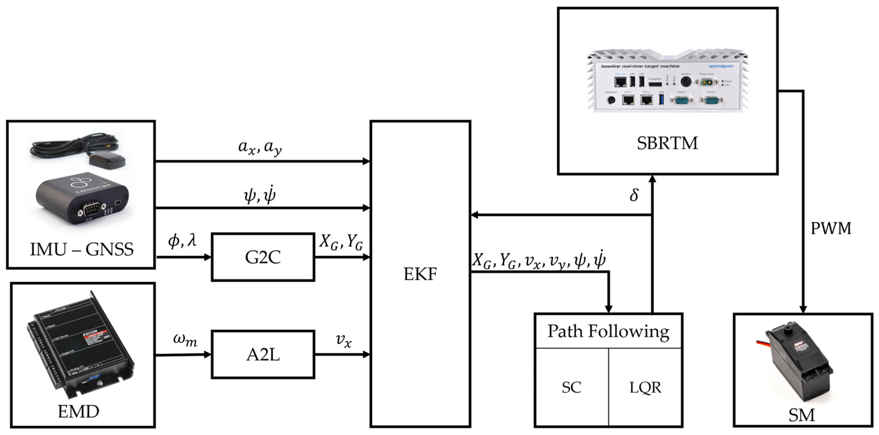
Figure 2 illustrates the overall signal flow, from data acquisition (IMU—GNSS, EMD) to the steering system, actuated by SM. The acquired signals are processed in real time within the estimator (EKF) and control subsystems (SC and LQR), implemented in the SBRTM.

Figure 2. Hardware and software architecture of the control layout implemented on the vehicle platform.

The IMU provides longitudinal and lateral acceleration components in the vehicle reference frame $a_x$ and $a_y$, the orientation around the $Z$ axis $\psi$, and its rate $\dot{\psi }$. The GNSS module supplies the vehicle position in the geodetic reference frame, defined by the latitude $\varphi$, longitude $\lambda$, and altitude $h$. These quantities are converted into the global Cartesian reference system $(X_G,Y_G)$ through a custom Geodetic-to-Cartesian (G2C) converter, based on a standard ellipsoidal Earth model. The longitudinal velocity $v_x$, oriented along the $X$ axis, is obtained from the electric motor speed ${\omega }_m$, which is regulated by the EMD. The relation, described in Equation (A1) in Appendix A.1 and implemented through the Angular-to-Longitudinal (A2L) block, defines the conversion from ${\omega }_m$ to $v_x$.

To obtain accurate and time-consistent estimates of the vehicle dynamic states, the EKF is designed to unify the information provided by sensors at different sampling rates. By fusing IMU and GNSS data, it provides noise-filtered estimates of position, velocity, and orientation. In addition, it also computes an estimation of the lateral velocity $v_y$, directed along the $Y$ axis of the vehicle reference frame, which is not directly measured. These estimated states are then used by the SC and the LQR to generate the steering command $\delta$ required for the trajectory tracking. The covariance matrices of the EKF are identified by an optimization process in simulation, exploiting an equivalent 8-degrees-of-freedom (8-DoF) vehicle model.

3.1. Vehicle State Estimation

The state estimator used to enhance the accuracy of the vehicle measurements is an EKF, i.e., a nonlinear extension of the simple Kalman Filter (KF) capable of handling systems affected by strong nonlinearities [51,52]. This algorithm can perform an estimation starting from the combination of a mathematical model, expressed in the state space, Equation (1), with noisy sensor measurements, Equation (2), through two sequential phases, prediction and correction. In the prediction step, the filter propagates the current state estimation according to the process model, while in the correction step, the real measurements are used to refine the estimation

In the prediction step, the system states ${\mathit{x}}_k$ at time step $k$ are evaluated as a nonlinear function $f$ of the states ${\mathit{x}}_{k-1}$ and the inputs ${\mathit{u}}_{k-1}$ at the previous $k-1$ step by step, Equation (1),

$${\mathit{x}}_k=f\left({\mathit{x}}_{k-1},{\mathit{u}}_{k-1}\right)+{\mathit{w}}_{k-1}$$

(1)

where ${\mathit{w}}_{k-1}$ represents the process noises evaluated at the time step $k-1$.

The measurements ${\mathit{z}}_k$ are expressed as a nonlinear function $g$ of the states ${\mathit{x}}_k$ by Equation (2),

$${\mathit{z}}_k=g\left({\mathit{x}}_k\right)+{\mathit{v}}_k$$

(2)

where ${\mathit{v}}_{\mathit{k}}$ denotes the measurement noise vector.

3.1.1. EKF Process Model

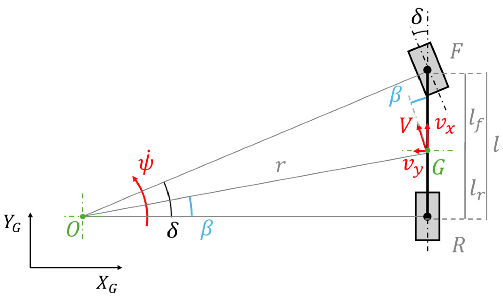
In this estimator, a kinematic bicycle model, illustrated in Figure 3, is used to represent the vehicle as a single-track system with front-wheel steering [53,54]. This simplified vehicle representation provides a good balance between physical accuracy and computational efficiency, which is crucial for real-time applicability on the scaled platform. Moreover, the lack of detailed tire data in the kinematic model prevents the use of a more complex dynamic formulation.

Figure 3. Kinematic bicycle model implemented in the EKF for vehicle state estimation.

The kinematic bicycle system assumes that the velocity vectors at the front and rear wheels are perfectly aligned with the wheel mid-plane, implying zero longitudinal and lateral tire slip. This approximation can be considered valid at low speeds, where lateral tire forces remain small [53].

In the kinematic bicycle model:

• $G$ is the Center of Gravity (CoG);
• $O$ is the center of curvature;
• $F, R$ indicate the front and rear axles;
• $l$ is the wheelbase;
• $l_f$ is the distance between $G$ and the front axle $F$;
• $l_r$ is the distance between $G$ and the rear axle $R$;
• $r$ is the distance between $G$ and $O$, namely the radius of the curvature;
• $V$ is the vehicle speed;
• $\beta$ is the sideslip angle, i.e., the angle between $V$ and $v_x$.

In Equation (1), the system state is represented by the vector $\mathit{x}={\left[X_G,Y_G,v_x,v_y,\psi ,\dot{\psi }\right]}^T$ while the inputs are $\mathit{u}={\left[\delta , a_x,a_y\right]}^T$. It is important to remark that $\delta$ is the only actual control input of the real vehicle, whereas $a_x$ and $a_y$ are measured inputs provided by the IMU. To simplify the EKF formulation, these accelerations are included in the kinematic bicycle process model, Equation (1), as inputs, even though they are not physically commanded. The measurements matrix $\mathit{z}=\left[{\mathit{Y}}_{GNSS}, {\mathit{Y}}_{IMU}\right]$ includes measurements coming from the GNSS, ${\mathit{Y}}_{GNSS}=\left[X_G,Y_G\right]$ and from the IMU, including the estimated vehicle speed, ${\mathit{Y}}_{IMU}=\left[v_x,\psi ,\dot{\psi }\right]$.

The state equations $f$ are expressed in Equations (3)–(9). In detail, Equations (3) and (4) describe the velocity components in the global reference frame. Equations (5)–(8) provide the vehicle kinematics in the local body-fixed reference frame, while Equation (9) expresses the vehicle speed magnitude from its components.

$${\dot{X}}_G=V\cos (\beta +\psi )$$

(3)

$${\dot{Y}}_G=V\sin (\beta +\psi )$$

(4)

$${\dot{v}}_x=v_y\dot{\psi }+a_x$$

(5)

$${\dot{v}}_y=-v_x\dot{\psi }+a_y$$

(6)

$$\dot{\psi }={\displaystyle \frac{V}{l}}\tan \delta \cos \beta$$

(7)

$$\ddot{\psi }=0$$

(8)

$$V=\sqrt{v_x^2+v_y^2}$$

(9)

3.1.2. EKF Covariances Tuning

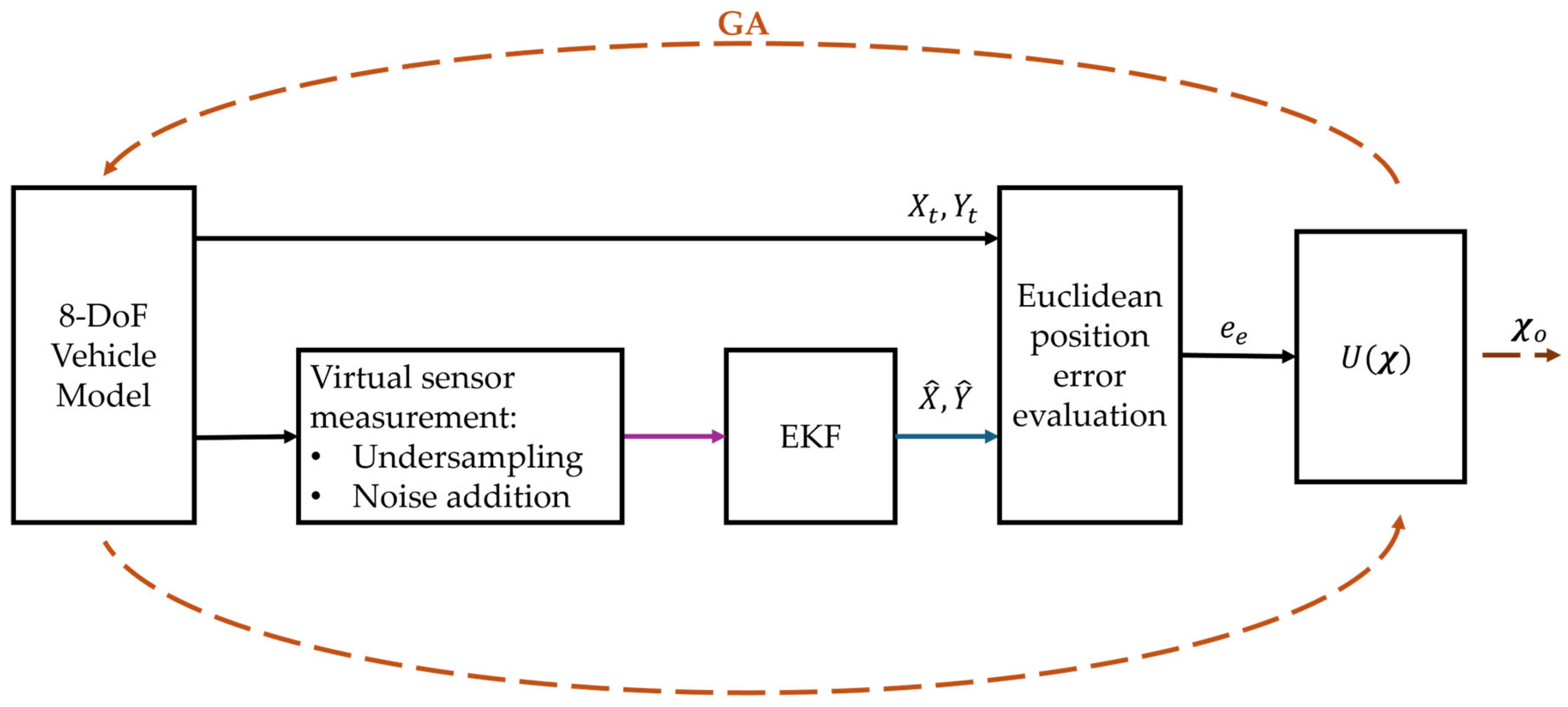
The tuning of the EKF process covariance matrix ($Q$) is carried out in simulation through an optimization procedure. A Genetic Algorithm (GA) is adopted for this task, since its stochastic nature enables an effective exploration of the parameter space and reduces the risk of converging to local minima. The objective is to minimize the discrepancy between the EKF-estimated states and the ground-truth data generated by an 8-degrees-of-freedom vehicle model. The latter includes longitudinal and lateral translations, roll and yaw rotations, and the rotational dynamics of the four wheels. Its outputs are under sampled and corrupted with white noise to emulate the behavior of the real sensors.

Figure 4 illustrates the schematic workflow of the GA-based optimization procedure adopted for the tuning of the EKF process covariance matrix. The diagram shows the generation of ground-truth data from the 8-DoF vehicle model, the creation of virtual sensor measurements, the EKF estimation, the evaluation of the error, and the cost function creation, used to guide the GA towards the optimal covariance values.

Figure 4. Schematic representation of the GA-based optimization procedure adopted for tuning the EKF process covariance matrix.

The simulated maneuvers consist of a $100°$ ramp steer, followed by a $20°$ sweep steer (frequency of $2$ Hz in $10$ s) at $15$ km/h. The measurement-noise covariance matrices adopted for the GNSS and IMU channels are fixed according to the sensor specifications and are reported in Table A1 of Appendix A.2.

The multi-variable optimization problem handled by the GA is formulated in Equation (10):

$${\mathsf{\chi }}_o=\mathrm{a}\mathrm{r}\mathrm{g}\min U\left(\mathsf{\chi }\right) : \underset{\_}{\mathsf{\chi }}\le \mathsf{\chi }\le \stackrel{-}{\mathsf{\chi }}\subseteq {\mathbb{R}}^n$$

(10)

where $\mathsf{\chi }$ represents the set of variables to be tuned, $U\left(\mathsf{\chi }\right)$ is the cost function, ${\mathsf{\chi }}_o$ is the optimal set of variables. The optimization is constrained by lower and upper bounds, indicated by $\underset{\_}{\mathsf{\chi }}$ and $\stackrel{-}{\mathsf{\chi }}$, which define the admissible range for each parameter.

The cost function combines the maximum and the RMS of the Euclidean position error $e_e$, as reported in Equations (11) and (12):

$$U\left(\mathsf{\chi }\right)=\alpha \max \left(e_e\right)+\left(1-\alpha \right) \mathrm{R}\mathrm{M}\mathrm{S}\mathrm{E}\left(e_e\right)$$

(11)

$$e_e=\sqrt{(X_t-\widehat{X}{)}^2+(Y_t-\widehat{Y}{)}^2}$$

(12)

where $(X_t,Y_t)$ are the ground-truth trajectory coordinates, $(\widehat{X},\widehat{Y})$ the EKF estimates, and $\alpha =0.6$ is a weighting parameter. The $\max \left(e_e\right)$ term is the maximum value of this error over the entire maneuver and $\mathrm{R}\mathrm{M}\mathrm{S}\mathrm{E}\left(e_e\right)$ is the root mean square error.

The optimization process starts with a randomly generated initial population and stops after $60$ generations.

The resulting optimal process covariance matrix is reported in Table A1 of Appendix A.2.

3.2. Stanley Controller

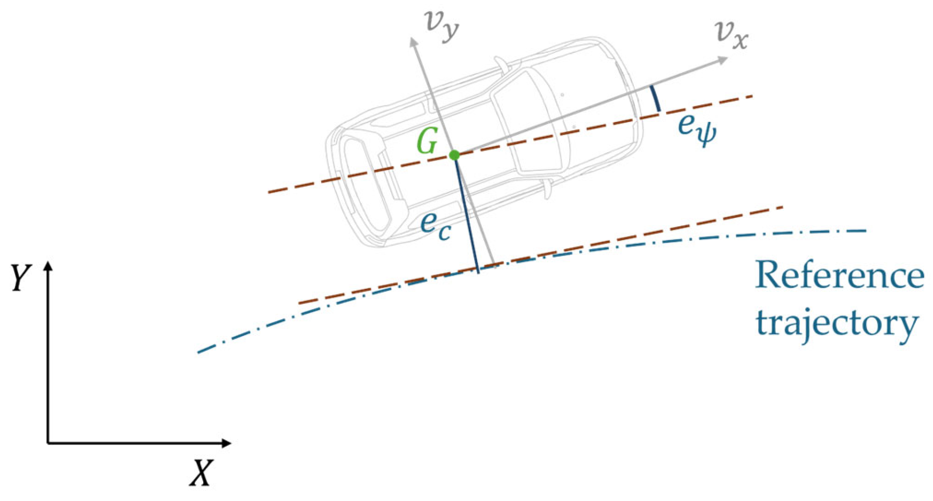
The SC is a geometric path-tracking algorithm commonly employed in autonomous driving applications [55]. Thanks to its simplicity, robustness, and reduced computational demand, it is particularly suitable for real-time implementation on scaled vehicle platforms. This controller determines the steering angle $\delta$ based on the cross-track error $e_c$, and the heading error $e_{\psi }$. As shown in Figure 5, $e_c$ is defined as the perpendicular distance between the vehicle position and the desired path, while $e_{\psi }$ corresponds to the angular deviation between the vehicle orientation and the tangent to the reference trajectory.

Figure 5. Geometric definition of the cross-track and heading errors used in the path-following controllers.

The reference trajectory ($X_r,{ Y}_r$) and orientation (${\psi }_r$) are provided as input to the SBRTM and used as a basis for computing $e_c$ and $e_{\psi }$ from the actual vehicle global position $(X_G,{ Y}_G)$ and yaw angle ($\psi$) estimated by the EKF. The analytical expressions of $e_c$ and $e_{\psi }$ are reported in Equations (A2) and (A3) in Appendix A.3.

$\delta$ is computed according to Equation (13) as the weighted sum of the heading error and the lateral deviation from the reference trajectory. The selection of the gain $k_e$ is crucial for ensuring stable tracking performance: excessively low values lead to slow convergence, while overly high values can induce oscillatory behavior; the selected value is reported in Table A2 within Appendix A.3.

$$\delta =e_{\psi }+\mathrm{atan}\left({\displaystyle \frac{k_e{e}_c}{v_x}}\right)$$

(13)

3.3. LQR Controller

The LQR is a state-feedback control law derived from optimal control theory [56]. The algorithm determines the optimal control input $u\left(t\right)$ by minimizing a quadratic cost function $J$, reported in Appendix A.4, Equation (A4). The resulting state-feedback law is expressed in Equation (14).

$$u\left(t\right)=-\mathit{K}\mathit{x}\left(t\right)$$

(14)

where $\mathit{K}$ is the feedback gain matrix and $\mathit{x}\left(t\right)$ denotes the state vector.

Equation (15) reports the Algebraic Riccati Equation, whose solution is used to compute the feedback gain $\mathit{K}$.

$$\mathit{K}=R^{-1}{\mathit{B}}^{T}P$$

(15)

where $R$ is a scalar weight penalizing the control effort, $\mathit{B}$ is the input matrix of the system and $P$ is the solution of the Algebraic Riccati Equation (ARE). The value of $\mathit{K}$ is reported in Table A3 in Appendix A.4.

In this study, the LQR is designed based on the Dynamic Single-Track Error (DSTE) model as expressed in Equation (16). The cost function is formulated with respect to the trajectory-tracking performance, following the approach demonstrated by Bui et al. and Yang [57,58]. The state vector $\mathit{e}=[e_y,e_{\psi },{\dot{e}}_y,{\dot{e}}_{\psi }{]}^T$ includes the lateral error $e_y$, the relative yaw error $e_{\psi }$, and their time derivatives ${\dot{e}}_y$ and ${\dot{e}}_{\psi }$, whose analytical expressions are reported in Appendix A.4, Equations (A5) and (A6). The steering angle $\delta$ represents the control input $u$(t), while ${\dot{\psi }}_r$ denotes the reference yaw rate. The matrices ${\mathit{A}}_{\mathit{e}}$, ${\mathit{B}}_{\delta }$, and ${\mathit{B}}_{\psi }$ define, respectively, the system dynamics, the influence of $\delta$, and the contribution of ${\dot{\psi }}_r$ to the evolution of the error states.

All vehicle parameters used for the controller synthesis are reported in Table A4 in Appendix A.4, and a detailed formulation of matrices ${\mathit{A}}_{\mathit{e}}$, ${\mathit{B}}_{\delta }$, and ${\mathit{B}}_{\psi }$, is provided in Appendix A.4, Equations (A7)–(A9), as well.

$$\dot{\mathit{e}}={\mathit{A}}_{\mathit{e}}\mathit{e}+{\mathit{B}}_{\delta }\delta +{\mathit{B}}_{\psi }{\dot{\psi }}_r$$

(16)

4. Test Procedure and Data Processing

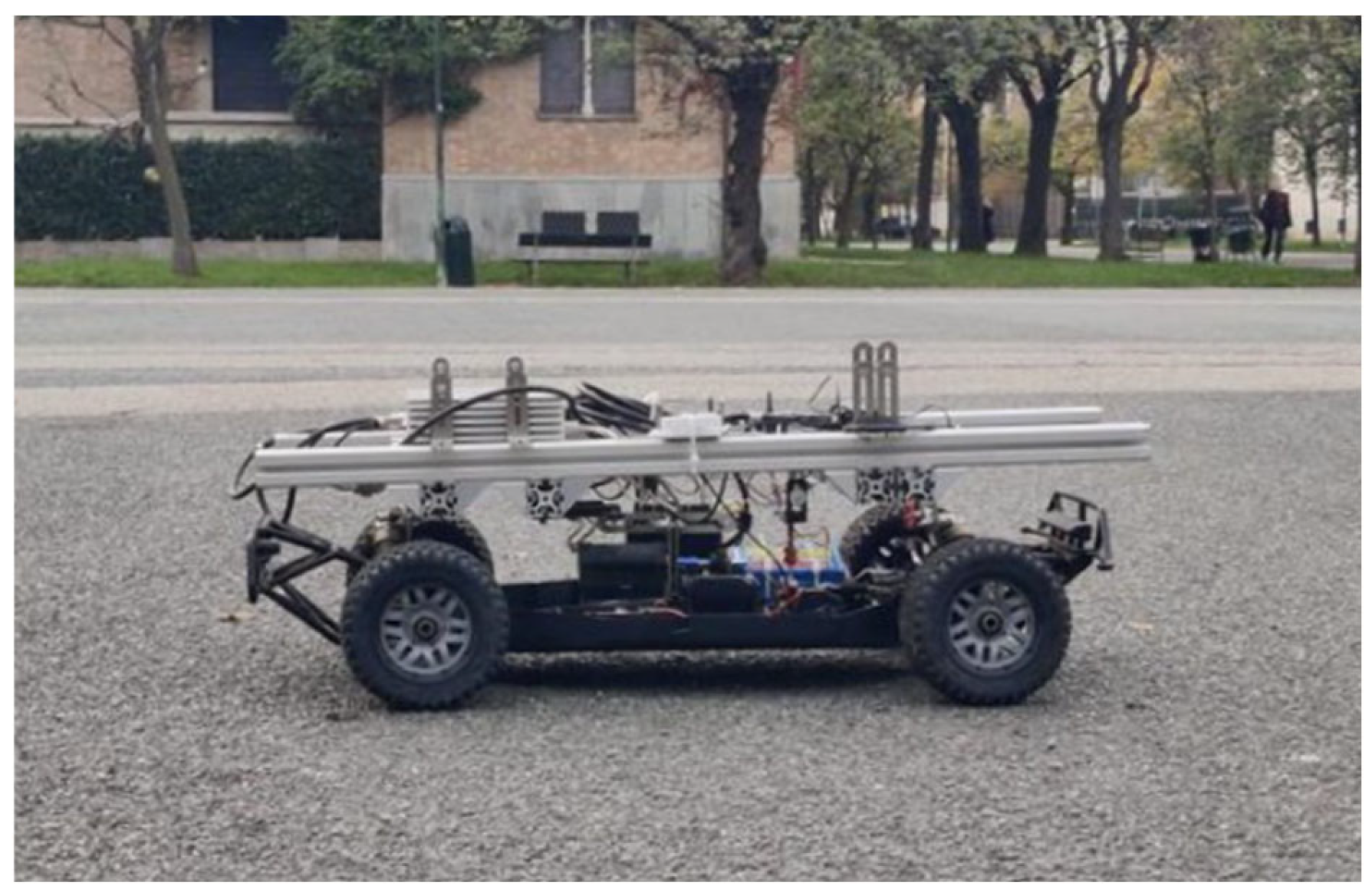
An experimental campaign is conducted to assess the performance of both the state estimator and the path-following controllers. Figure 6 shows the $1:5$ scale vehicle ready for the outdoor test campaign.

Figure 6. The $1:5$ scale vehicle during the outdoor experimental test.

Two reference trajectories are performed at constant speed:

• The first maneuver consists of a $6$ m-radius circular path, in a counterclockwise direction at $6$ km/h;
• The second maneuver is a figure-eight path composed of two adjacent $6$ m-radius circles, the first counterclockwise and the second clockwise, carried at $4$ km/h.

The circular trajectory serves to assess the controllers’ performance under steady-state, constant-curvature conditions, whereas the figure-eight trajectory imposes alternating curvature and short-duration transient dynamics to examine each controller’s capability in managing rapid variations in lateral acceleration and yaw rate. Each test case is repeated three times to check the robustness.

All experimental data are synchronously logged during each run and postprocessed in MATLAB. High-frequency experimental noise components are attenuated using a second-order low-pass Butterworth filter [59] with a cut-off frequency of $10$ Hz.

For each combination of maneuver and controller, Key Performance Indicators (KPIs) are evaluated over the entire test duration, excluding short transient phases at the beginning and end of each run. The metrics adopted for the comparison are the maximum ($\mathrm{M}\mathrm{a}\mathrm{x}$), average ($\mathrm{M}\mathrm{e}\mathrm{a}\mathrm{n}$), and Standard Deviation ($\mathrm{S}\mathrm{t}\mathrm{d}$) of both the cross-track $e_c$ and heading errors $e_{\psi }$. Since the LQR does not compute $e_c$ internally, this quantity is obtained during postprocessing. The $\mathrm{M}\mathrm{a}\mathrm{x}$ value represents the peak magnitude of the error, with its original sign.

5. Results

This section presents the results obtained from experimental tests. A comparative analysis between the two controllers is provided, aiming to assess their accuracy and robustness under real-world operating conditions.

5.1. Circular Trajectory

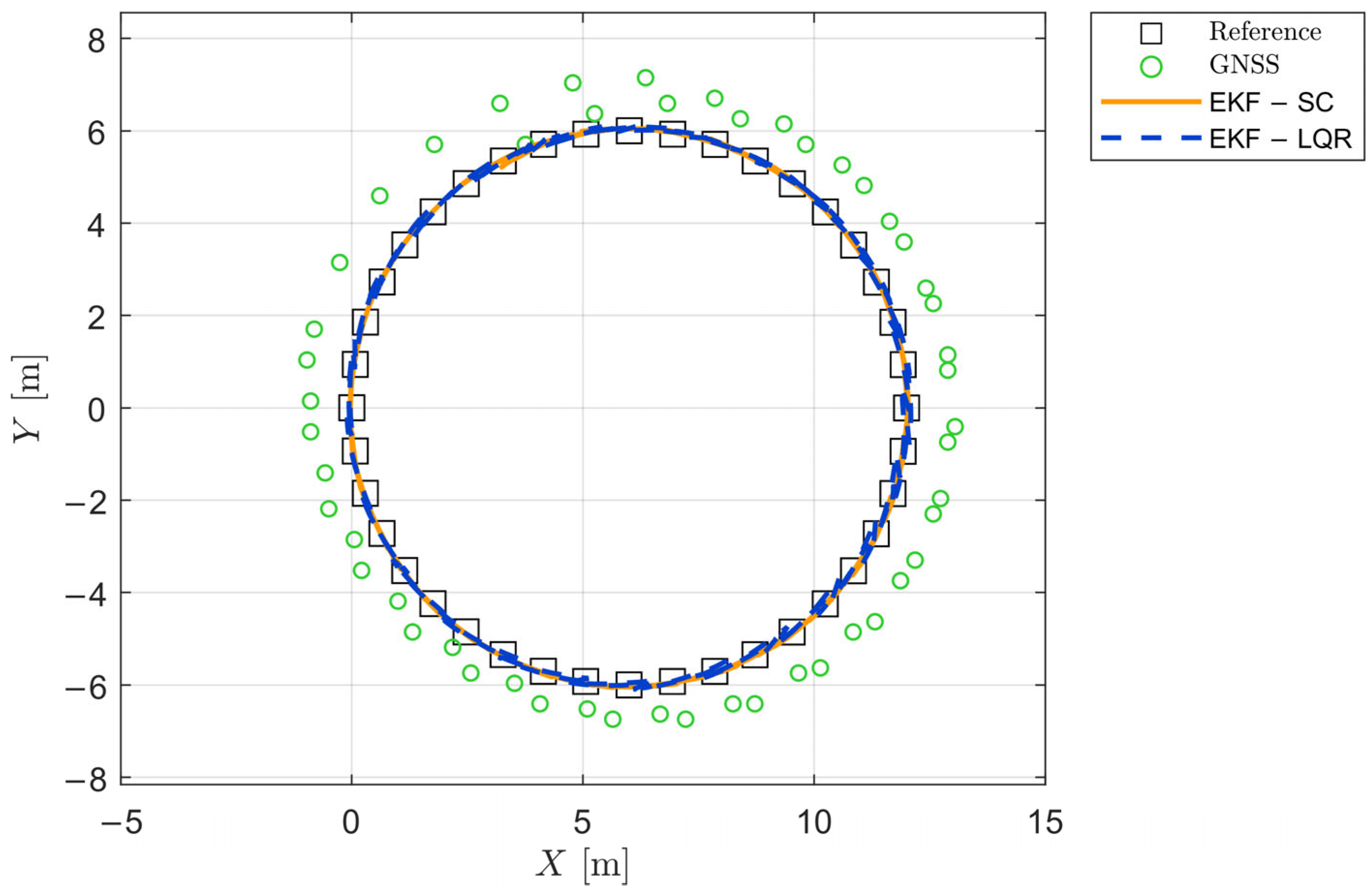
Figure 7 illustrates the comparison between the reference circular path (black squares), the raw GNSS measurements (green circles), and the experimental trajectories obtained with the two controllers, EKF–SC (orange solid line) and EKF–LQR (blue dashed line). The color and line-style convention adopted in this Figure is maintained throughout all the plots in this section. According to Figure 7, a slight offset is visible among the raw GNSS data and the reference trajectory, yet it is consistently corrected in the estimated trajectories.

Figure 7. Comparison between the reference circular trajectory, the raw GNSS data, and the experimental trajectories obtained with the SC and the LQR at $6$ km/h.

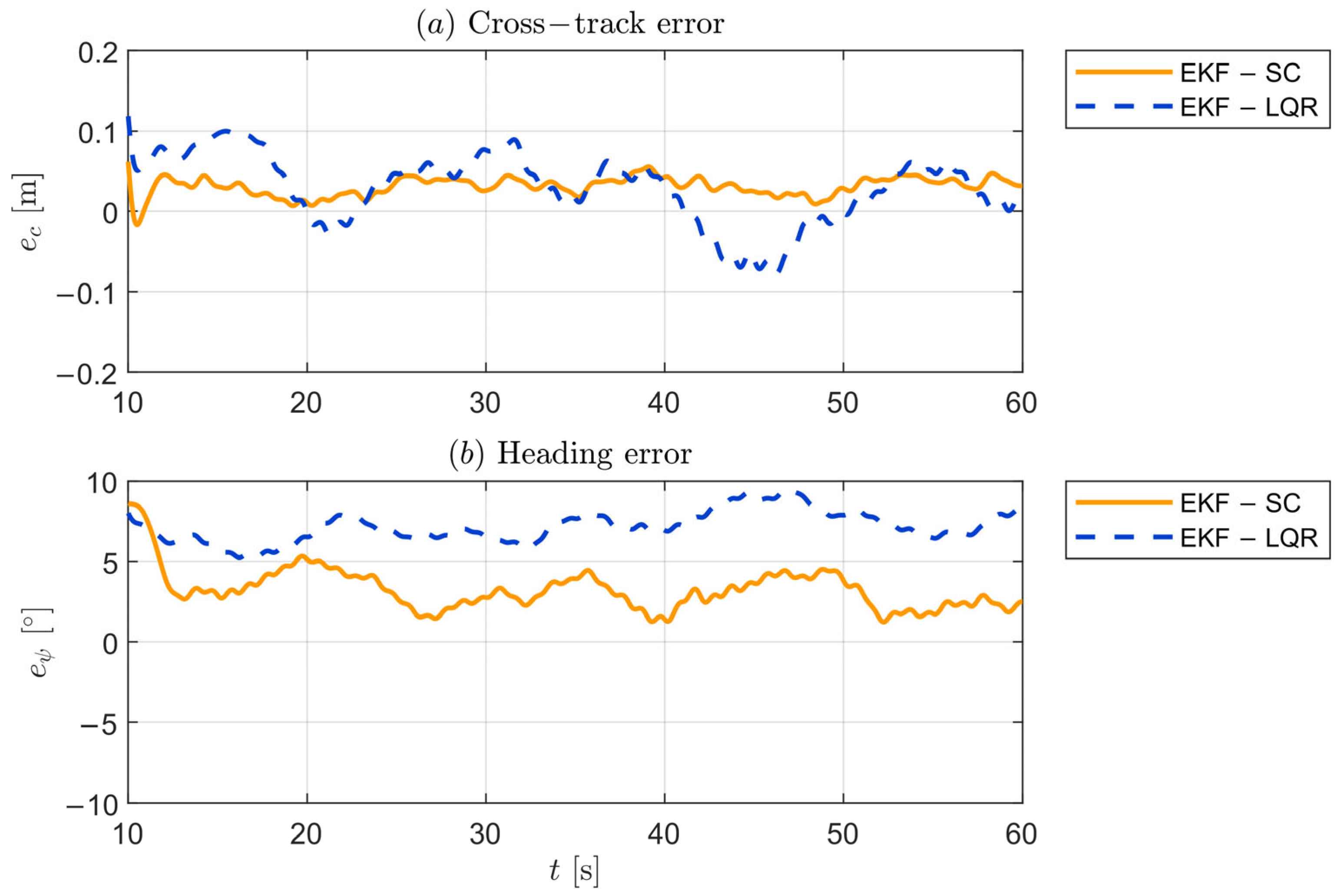
Figure 8 reports the time histories of the control errors, $e_c$ and $e_{\psi }$, during the circular trajectory, while the corresponding KPIs are listed in Table 1. Maximum, mean, and standard deviation of the $e_c$ and $e_{\psi }$ errors obtained during the circular trajectory test at $6$ km/h. The SC achieves smaller cross-track deviations and lower peak amplitudes, ranging from $+0.06$ m to $-0.02$ m, compared with $+0.12$ m to $-0.08$ m for the LQR. The SC $e_c$ maximum deviation is therefore halved with respect to the LQR ($0.06$ m vs. $0.12$ m), the mean error is lower as well ($0.03$ m vs. $0.04$ m). Lastly, the standard deviation is still lower for the SC ($0.01$ m vs. $0.04$ m). Regarding the heading error $e_{\psi }$, the LQR exhibits a gradual drift over time, resulting in a higher maximum ($9.53°$ vs. $8.61°$) and mean value ($7.16°$ vs. $3.24°$), although associated with a smaller standard deviation compared to the SC ($0.96°$ vs. $1.28°$).

Figure 8. Time histories of the cross-track and heading errors during the circular trajectory at $6$ km/h.

Table 1. Maximum, mean, and standard deviation of the $e_c$ and $e_{\psi }$ errors obtained during the circular trajectory test at $6$ km/h.

Cross-Track Error
Controller	$\mathbf{M}\mathbf{a}\mathbf{x}$ [m]	$\mathbf{M}\mathbf{e}\mathbf{a}\mathbf{n}$ [m]	$\mathbf{S}\mathbf{t}\mathbf{d}$ [m]
SC	$0.06$	$0.03$	$0.01$
LQR	$0.12$	$0.04$	$0.04$
Heading error
Controller	$\mathbf{M}\mathbf{a}\mathbf{x}$ [°]	$\mathbf{M}\mathbf{e}\mathbf{a}\mathbf{n}$ [°]	$\mathbf{S}\mathbf{t}\mathbf{d}$ [°]
SC	$8.61$	$3.24$	$1.28$
LQR	$9.53$	$7.16$	$0.96$

The magnitude of the errors remains limited throughout the maneuver, indicating the absence of sharp discrepancies between the two controllers. The SC demonstrates faster convergence towards the reference path, whereas the LQR ensures smoother steering actions. Both controllers exhibit robust and stable performance along the entire circular trajectory.

5.2. Figure-Eight Trajectory

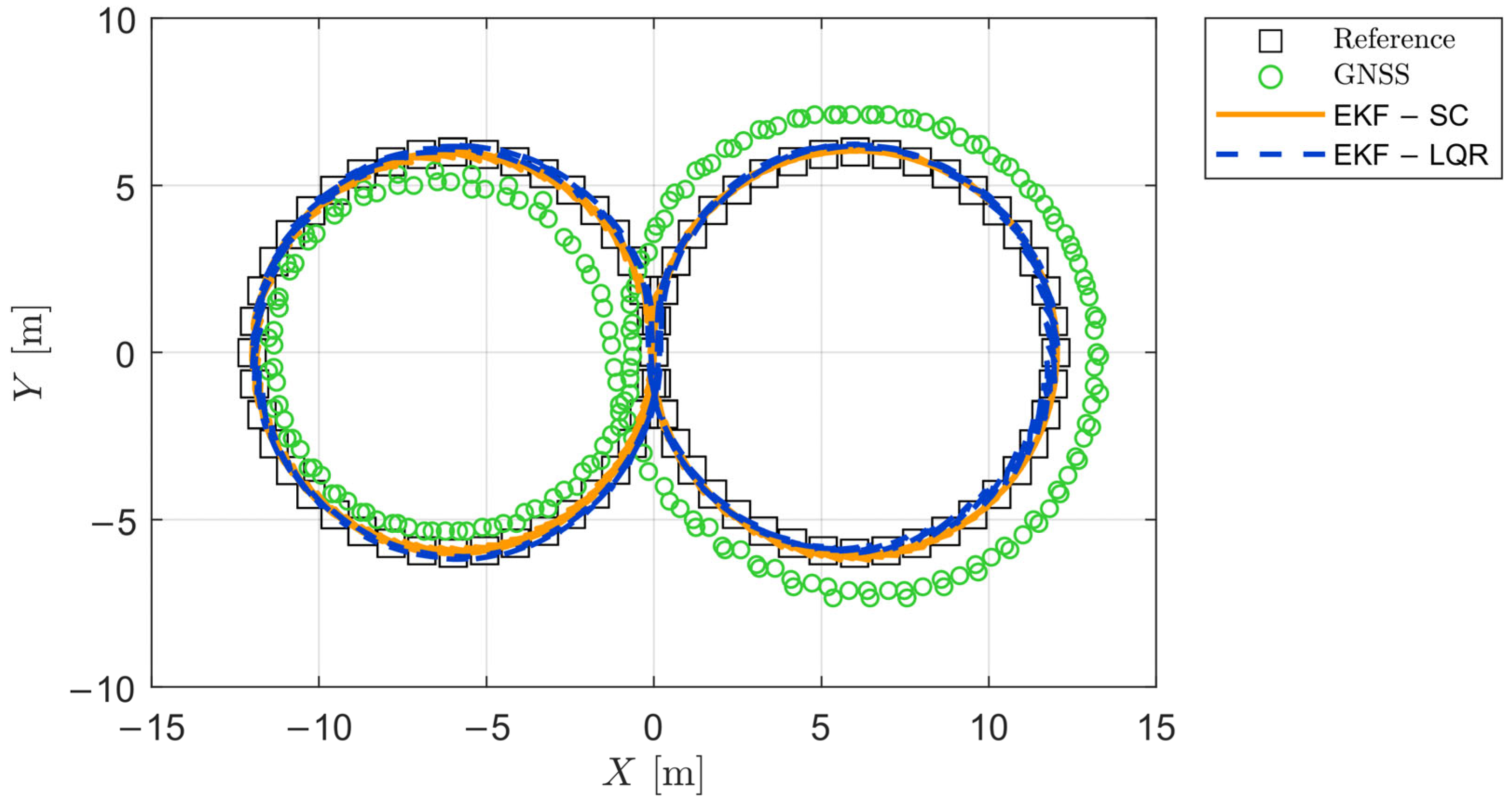
The figure-eight reference trajectory, the raw GNSS measurements, and the experimental results obtained with the EKF–SC and EKF–LQR are illustrated in Figure 9. As already observed in the circular trajectory, the apparent offset among GNSS data and reference trajectory is effectively handled by both controllers.

Figure 9. Comparison between the reference figure-eight trajectory, the raw GNSS data, and the experimental trajectories obtained with the SC and the LQR at $4$ km/h.

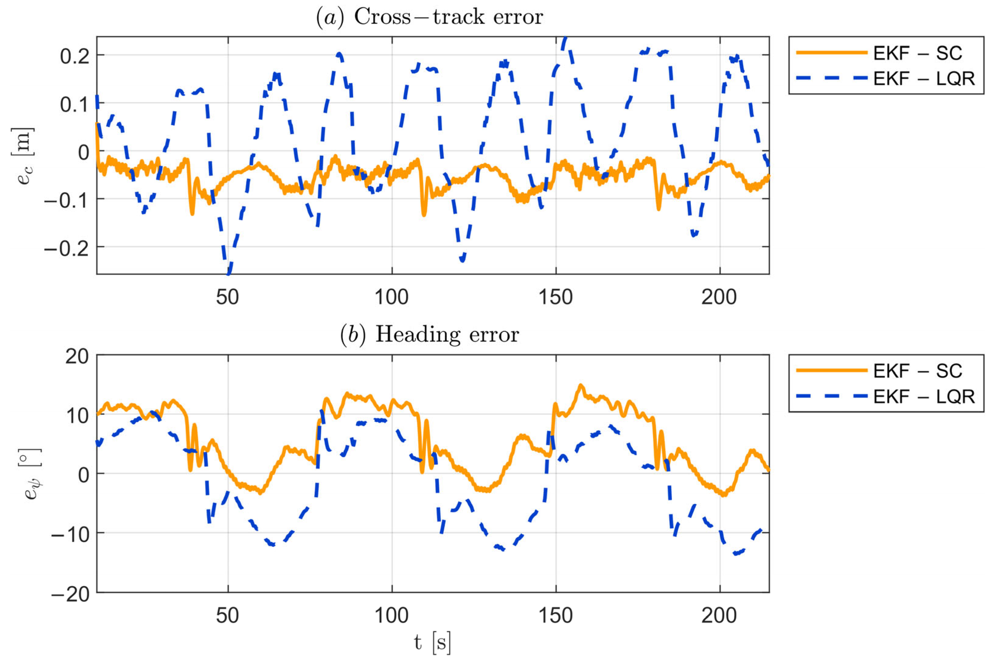
Figure 10 reports the time histories of the control errors, $e_c$ and $e_{\psi }$, during the figure-eight trajectory, while the corresponding KPIs are listed in Table 2. The SC approximately halves the maximum $e_c$ magnitude, compared to the LQR ($-0.13$ m vs. $-0.26$ m) and exhibits a remarkably lower standard deviation, about 80% smaller ($0.02$ m vs. $0.11$ m). The mean values of both controllers are comparable, although the LQR shows a slightly lower value ($-0.03$ m vs. $-0.05$ m). Conversely, regarding the heading error $e_{\psi }$, the LQR exhibits a smaller absolute maximum ($13.60°$ vs. $16.89°$) and mean values ($-1.05°$ vs. $5.64°$), while the SC achieves a lower standard deviation ($5.28°$ vs. $7.44°$). A similar stable behavior observed in the circular test is observed in this maneuver. The KPIs are summarized in Table 2.

Figure 10. Time histories of the cross-track and heading errors during the figure-eight trajectory at $4$ km/h.

Table 2. Maximum, mean, and standard deviation of the $e_c$ and $e_{\psi }$ errors obtained during the figure-eight trajectory test at $4$ km/h.

Cross-Track Error
Controller	$\mathbf{M}\mathbf{a}\mathbf{x}$ [m]	$\mathbf{M}\mathbf{e}\mathbf{a}\mathbf{n}$ [m]	$\mathbf{S}\mathbf{t}\mathbf{d}$ [m]
SC	$-0.13$	$-0.05$	$0.02$
LQR	$-0.26$	$-0.03$	$0.11$
Heading error
Controller	$\mathbf{M}\mathbf{a}\mathbf{x}$ [°]	$\mathbf{M}\mathbf{e}\mathbf{a}\mathbf{n}$ [°]	$\mathbf{S}\mathbf{t}\mathbf{d}$ [°]
SC	$16.89$	$5.64$	$5.28$
LQR	$-13.60$	$-1.05$	$7.44$

6. Conclusions

In this paper, two path-following control strategies, the Linear Quadratic Regulator and the Stanley controller, have been developed, implemented, and experimentally validated on a $1:5$ scale vehicle. The main outcomes of this research activity are summarized below:

• Extension of a previously developed scaled vehicle testbed: the modular and low-cost $1:5$ platform is upgraded with a high-precision IMU-GNSS module, enabling repeatable outdoor testing of autonomous driving algorithms;
• Development of an EKF-based estimator: the algorithm is employed to improve the accuracy of the vehicle states (position, velocity, and orientation) using data measured with different sampling rates. This goal is achieved by fusing high-frequency and noisy inertial data with low-frequency GNSS measurements;
• Experimental validation of path-following controllers: both the LQR and SC ensure accurate and repeatable trajectory tracking in the circular and figure-eight tests. The SC achieves higher lateral accuracy thanks to a more reactive lateral correction, as its proportional gain assigns a strong weight to the cross-track error $e_c$. Conversely, the LQR provides smoother and more stable yaw-error evolution, since it regulates the lateral and yaw errors and their time derivatives. This behavior becomes particularly evident in steady-state cornering, where the $e_{\psi }$ dynamics dominate. The results confirm the robustness and reliability of the proposed control and estimation framework under both steady-state and transient conditions, highlighting the effectiveness of the scaled vehicle testbed for the experimental validation of path-following algorithms;
• Platform suitability for control benchmarking: the proposed testbed proves effective for evaluating and comparing control strategies under outdoor conditions. It offers a cost-efficient alternative to full-scale vehicle and simulation testing, enabling robust and repeatable experimental assessment.

Future developments may focus on enhancing the experimental platform and broadening its testing capabilities. A first step could involve the integration of a dynamic vehicle model with tire-force representation within the EKF framework, enabling a more accurate estimation of lateral dynamics. In addition, the adoption of more advanced control strategies, such as Model Predictive Control (MPC) or robust control approaches, could further improve tracking performance under more demanding operating conditions. Finally, the integration of onboard vision sensors, such as cameras, could enable perception-based control and expand the versatility of the testbed toward more advanced autonomous driving applications, improving path planning capability and obstacle detection.

Appendix A.1

Equation (A1) defines the relationship used to compute the vehicle longitudinal velocity:

$$v_x={\omega }_m i_g r_w$$

(A1)

where $i_g=1/10.25$ is the transmission ratio and $r_w=0.090$ m is the wheel radius.

Appendix A.2

Table A1 reports the covariance values adopted in the EKF formulation.

Table A1. Summary of the EKF covariance matrices.

Quantity	Symbol	Value
GNSS measurement noise covariance	${\mathit{R}}_{\mathrm{G}\mathrm{N}\mathrm{S}\mathrm{S}}$	$\left[\begin{array}{cc}4& 0\\ 0& 4\end{array}\right]$
IMU measurement noise covariance	${\mathit{R}}_{\mathrm{I}\mathrm{M}\mathrm{U}}$	$\left[\begin{array}{ccc}0.1& 0& 0\\ 0& 0.01& 0\\ 0& 0& 1\end{array}\right]$
EKF process noise covariance	$\mathit{Q}$	$\left[\begin{array}{cccccc}1.2891·{10}^{-4}& 0& 0& 0& 0& 0\\ 0& 7.0360·{10}^{-4}& 0& 0& 0& 0\\ 0& 0& 0.0019& 0& 0& 0\\ 0& 0& 0& 7.0839& 0& 0\\ 0& 0& 0& 0& 8.1434·{10}^{-4}& 0\\ 0& 0& 0& 0& 0& 0.0848\end{array}\right]$

Table A1. Summary of the EKF covariance matrices.

Quantity	Symbol	Value
GNSS measurement noise covariance	${\mathit{R}}_{\mathrm{G}\mathrm{N}\mathrm{S}\mathrm{S}}$	$\left[\begin{array}{cc}4& 0\\ 0& 4\end{array}\right]$
IMU measurement noise covariance	${\mathit{R}}_{\mathrm{I}\mathrm{M}\mathrm{U}}$	$\left[\begin{array}{ccc}0.1& 0& 0\\ 0& 0.01& 0\\ 0& 0& 1\end{array}\right]$
EKF process noise covariance	$\mathit{Q}$	$\left[\begin{array}{cccccc}1.2891·{10}^{-4}& 0& 0& 0& 0& 0\\ 0& 7.0360·{10}^{-4}& 0& 0& 0& 0\\ 0& 0& 0.0019& 0& 0& 0\\ 0& 0& 0& 7.0839& 0& 0\\ 0& 0& 0& 0& 8.1434·{10}^{-4}& 0\\ 0& 0& 0& 0& 0& 0.0848\end{array}\right]$

Appendix A.3

The computation of the cross-track $e_c$ and heading $e_{\psi }$ errors is reported in Equations (A2) and (A3):

$$e_c=(Y_r-Y_G)\cos {\psi }_r-(X_r-X_G)\sin {\psi }_r$$

(A2)

$$e_{\psi }={\psi }_r-\psi$$

(A3)

where $(X_r,Y_r,{\psi }_r)$ are the position and orientation of the closest point on the reference trajectory, and $(X_G,Y_G,\psi )$ are the vehicle position and orientation in the global reference frame. The adopted sign convention assumes that $e_c>0$ when the vehicle lies to the right of the reference trajectory, and $e_{\psi }>0$ when $\psi$ is smaller than ${\psi }_r$.

In this work, the gain $k_e$ is set in accordance with [60], as it provided stable and accurate path tracking during the experimental tests. The adopted value is reported in Table A2.

Table A2. Stanley Controller gain.

Quantity	Symbol	Value
Stanley Controller gain	$k_e$	$5$

Table A2. Stanley Controller gain.

Quantity	Symbol	Value
Stanley Controller gain	$k_e$	$5$

Appendix A.4

The cost function considers both state deviations and control effort, as expressed in Equation (A4), where $\mathit{x}\left(t\right)$ denotes the state vector and $u\left(t\right)$ represents the control input.

$$J={\int }_0^{\mathrm{\infty }}\left({\mathit{x}\left(t\right)}^T{\mathit{Q}}_{LQR}\mathit{x}\right(t)+{\mathit{u}\left(t\right)}^T{\mathit{R}}_{LQR}u(t\left)\right) dt$$

(A4)

where ${\mathit{Q}}_{LQR}\in {\mathbb{R}}^{n\times n}$ is a symmetric, positive semi-definite matrix penalizing state deviations, and ${\mathit{R}}_{LQR}\in {\mathbb{R}}^{m\times m}$ is a symmetric, positive definite matrix penalizing control effort.

Table A3 reports the obtained value of the LQR feedback gain $\mathit{K}$.

Table A3. LQR feedback gain.

Quantity	Symbol	Value
LQR feedback gain	$\mathit{K}$	$\left[\begin{array}{cccc}0.4472& 0& 0& 0\\ 0& 0.9373& 0& 0\\ 0& 0& -0.0024& 0\\ 0& 0& 0& 0.0442\end{array}\right]$

Table A3. LQR feedback gain.

Quantity	Symbol	Value
LQR feedback gain	$\mathit{K}$	$\left[\begin{array}{cccc}0.4472& 0& 0& 0\\ 0& 0.9373& 0& 0\\ 0& 0& -0.0024& 0\\ 0& 0& 0& 0.0442\end{array}\right]$

The lateral error $e_y$ is obtained by integrating its time derivative, whereas the cross-track error $e_c$ is purely geometric quantity.

Based on the single-track geometry, the error rates can be expressed according to Equations (A5) and (A6):

$${\dot{e}}_y=v_y+v_x e_{\psi }$$

(A5)

$${\dot{e}}_{\psi }=\psi -{\dot{\psi }}_r$$

(A6)

The state-space matrices of the linearized DSTE model are reported in Equations (A7)–(A9). Matrix ${\mathit{A}}_{\mathit{e}}$ represents the vehicle lateral and yaw dynamics, while ${\mathit{B}}_{\delta }$ and ${\mathit{B}}_{\psi }$ describe the influence of the steering input and of the reference yaw rate, respectively.

$${\mathit{A}}_{\mathit{e}}=\left[\begin{array}{cccc}0& 0& 1& 0\\ 0& 0& 0& 1\\ 0& 2{\displaystyle \frac{C_f+C_r}{m}}& -2{\displaystyle \frac{C_f+C_r}{m{v}_x}}& -2{\displaystyle \frac{C_f{l}_f-C_r{l}_r}{m{v}_x}}\\ 0& 2{\displaystyle \frac{C_f{l}_f+C_r{l}_r}{J_z}}& -2{\displaystyle \frac{C_f{l}_f-C_r{l}_r}{J_z{v}_x}}& -2{\displaystyle \frac{C_f{l}_f^2+C_r{l}_r^2}{J_z{v}_x}}\end{array}\right]$$

(A7)

$${\mathit{B}}_{\delta }=\left[\begin{array}{c}0\\ 0\\ 2{\displaystyle \frac{C_f}{m}}\\ 2{\displaystyle \frac{c_f{l}_f}{J_z}}\end{array}\right]$$

(A8)

$${\mathit{B}}_{\psi }=\left[\begin{array}{c}0\\ 0\\ -v_x-2{\displaystyle \frac{C_f{l}_f-C_r{l}_r}{m{v}_x}}\\ -2{\displaystyle \frac{C_f{l}_f^2-C_r{l}_r^2}{J_z{v}_x}}\end{array}\right]$$

(A9)

Table A4 summarizes the parameters of the scaled vehicle used by the controllers.

Table A4. Scaled vehicle parameters.

Quantity	Symbol	Unit	Value
Mass	$m$	kg	$24.08$
Wheelbase	$l$	m	$0.61$
Front wheelbase	$l_f$	m	$0.34$
Rear wheelbase	$l_r$	m	$0.34$
Yaw moment of inertia	$J_z$	kg m2	$2.08$
Longitudinal velocity	$v_x$	m/s	$4.17$
Front cornering stiffness	$C_f$	N/rad	$27·{10}^3/60$
Rear cornering stiffness	$C_r$	N/rad	$20·{10}^3/60$

Table A4. Scaled vehicle parameters.

Quantity	Symbol	Unit	Value
Mass	$m$	kg	$24.08$
Wheelbase	$l$	m	$0.61$
Front wheelbase	$l_f$	m	$0.34$
Rear wheelbase	$l_r$	m	$0.34$
Yaw moment of inertia	$J_z$	kg m2	$2.08$
Longitudinal velocity	$v_x$	m/s	$4.17$
Front cornering stiffness	$C_f$	N/rad	$27·{10}^3/60$
Rear cornering stiffness	$C_r$	N/rad	$20·{10}^3/60$

The inertial and geometrical parameters are taken from a previously developed CAD model of the vehicle, while the cornering stiffnesses are estimated by scaling typical passenger-car data according to the vehicle mass ratio (≈1/60).

References

- Borneo, A.; Zerbato, L.; Miretti, F.; Tota, A.; Galvagno, E.; Misul, D.A. Platooning Cooperative Adaptive Cruise Control for Dynamic Performance and Energy Saving: A Comparative Study of Linear Quadratic and Reinforcement Learning-Based Controllers. Appl. Sci. 2023, 13, 10459. [Google Scholar] [CrossRef]
- Vella, A.D.; Biondo, L.; Tota, A.; Vigliani, A. Electrification and Control of a 1:5 Scale Vehicle for Automotive Testing Methodologies; SAE Technical Paper 2024-01-2271; SAE: Detroit, MI, USA, 2024. [Google Scholar] [CrossRef]
- Zein, Y.; Darwiche, M.; Mokhiamar, O. GPS Tracking System for Autonomous Vehicles. Alex. Eng. J. 2018, 57, 3127–3137. [Google Scholar] [CrossRef]
- Domberg, F.; Wembers, C.C.; Patel, H.; Schildbach, G. Deep Drifting: Autonomous Drifting of Arbitrary Trajectories Using Deep Reinforcement Learning. In Proceedings of the 2022 International Conference on Robotics and Automation (ICRA), Philadelphia, PA, USA, 23–27 May 2022; IEEE: New York, NY, USA, 2022; pp. 7753–7759. [Google Scholar]
- Masello, L.; Castignani, G.; Sheehan, B.; Murphy, F.; McDonnell, K. On the Road Safety Benefits of Advanced Driver Assistance Systems in Different Driving Contexts. Transp. Res. Interdiscip. Perspect. 2022, 15, 100670. [Google Scholar] [CrossRef]
- Bui, D.-T.; Nguyen, H.D.; Gu, Z.; Eichberger, A. Validation of Adaptive Cruise Control Based on Model Predictive Control for Autonomous Vehicles in Real-Time System. In Proceedings of the 2024 10th International Conference on Control, Decision and Information Technologies (CoDIT), Vallette, Malta, 1–4 July 2024; pp. 2621–2626. [Google Scholar]
- Souders, D.J.; Best, R.; Charness, N. Valuation of Active Blind Spot Detection Systems by Younger and Older Adults. Accid. Anal. Prev. 2017, 106, 505–514. [Google Scholar] [CrossRef]
- Jahoda, P.; Cech, J.; Matas, J. Autonomous Car Chasing. In Computer Vision–ECCV 2020 Workshops; Bartoli, A., Fusiello, A., Eds.; Springer International Publishing: Cham, Switzerland, 2020; pp. 337–352. [Google Scholar]
- De Cristofaro, F.; Lex, C.; Hu, J.; Eichberger, A. Lane Change Intention Prediction of Two Distinct Populations Using a Transformer. arXiv 2025, arXiv:2509.06529. [Google Scholar] [CrossRef]
- Tota, A.; Velardocchia, M.; Güvenç, L. Path Tracking Control for Autonomous Driving Applications. In Advances in Service and Industrial Robotics: In Proceedings of the 26th International Conference on Robotics in Alpe-Adria-Danube Region, RAAD 2017, Torino, Italy; Tota, A., Velardocchia, M., Güvenç, L., Eds.; Mechanisms and Machine Science; Springer International Publishing: Cham, Switzerland, 2017; Volume 49, p. 456. ISBN 978-3-319-61275-1. [Google Scholar]
- Kirovskii, O. Determination of Validation Testing Scenarios for an ADAS Functionality: Case Study; SAE International: Warrendale, PA, USA, 2019. [Google Scholar]
- Son, T.D.; Hubrechts, J.; Awatsu, L.; Bhave, A.; Van der Auweraer, H. A Simulation-Based Testing and Validation Framework for ADAS Development. In Proceedings of the 7th Transport Research Arena (TRA 2018), Vienna, Austria, 16–19 April 2018; Zenodo: Vienna, Austria, 2018. [Google Scholar]
- Xie, Z.; Ramezani, M.; Levinson, D. Reduced-Scale Mobile Robots for Autonomous Driving Research. IEEE Trans. Intell. Transp. Syst. 2024, 25, 15367–15387. [Google Scholar] [CrossRef]
- Lampe, N.; Ziaukas, Z.; Westerkamp, C.; Jacob, H.-G. Analysis of the Potential of Onboard Vehicle Sensors for Model-Based Maximum Friction Coefficient Estimation. In Proceedings of the 2023 American Control Conference (ACC), San Diego, CA, USA, 31 May–2 June 2023; IEEE: San Diego, CA, USA, 2023; pp. 1622–1628. [Google Scholar]
- Paul, D.; Velenis, E.; Cao, D.; Dobo, T. Optimalμ–Estimation-Based Regenerative Braking Strategy for an AWD HEV. IEEE Trans. Transp. Electrif. 2017, 3, 249–258. [Google Scholar] [CrossRef]
- Ribeiro, A.M.; Koyama, M.F.; Moutinho, A.; De Paiva, E.C.; Fioravanti, A.R. A Comprehensive Experimental Validation of a Scaled Car-like Vehicle: Lateral Dynamics Identification, Stability Analysis, and Control Application. Control Eng. Pract. 2021, 116, 104924. [Google Scholar] [CrossRef]
- Vella, A.D.; Tota, A.; Vigliani, A. On the Road Profile Estimation from Vehicle Dynamics Measurements; SAE Technical Paper 2021-01-1115; SAE: Grand Rapids, MI, USA, 2021. [Google Scholar] [CrossRef]
- Kumar, S.; Pasumarthy, R.; Bhatt, N. DEFT–A Scaled Electric Vehicle Platform for Testing Autonomous Driving Algorithm. TechRxiv 2024. [Google Scholar] [CrossRef]
- Becker, D.; Konthala, S.; Eckstein, L. Open-Source Tool Based Framework for Automated Performance Evaluation of an AD Function. In Proceedings of the III. International Conference on Electrical, Computer and Energy Technologies (ICECET 2023), Cape Town, South Africa, 16–17 November 2023; pp. 1–6. [Google Scholar]
- Caleffi, F.; Rodrigues, L.D.S.; Stamboroski, J.D.S.; Pereira, B.M. Small-Scale Self-Driving Cars: A Systematic Literature Review. J. Traffic Transp. Eng. Engl. Ed. 2024, 11, 271–292. [Google Scholar] [CrossRef]
- Gao, L.; Bai, W.; Leary, R.; Varadarajan, K.; Brennan, S. ROS Integration of External Vehicle Motion Simulations with an AIMSUN Traffic Simulator as a Tool to Assess CAV Impacts on Traffic. IFAC-PapersOnLine 2021, 54, 870–875. [Google Scholar] [CrossRef]
- Tajalli, M.; Niroumand, R.; Hajbabaie, A. Distributed Cooperative Trajectory and Lane Changing Optimization of Connected Automated Vehicles: Freeway Segments with Lane Drop. Transp. Res. Part C Emerg. Technol. 2022, 143, 103761. [Google Scholar] [CrossRef]
- Natvig, M.K.; Stav, E.; Stene, T.M. Concepts for Future Traffic Management Supporting Automation, Multimodal Coordination and Resilience. 2023. Available online: https://ssrn.com/abstract=4493781 (accessed on 30 October 2025).
- Tang, X.; Zhong, G.; Li, S.; Yang, K.; Shu, K.; Cao, D.; Lin, X. Uncertainty-Aware Decision-Making for Autonomous Driving at Uncontrolled Intersections. IEEE Trans. Intell. Transp. Syst. 2023, 24, 9725–9735. [Google Scholar] [CrossRef]
- Zeng, T.; Si, B. Mobile Robot Exploration Based on Rapidly-Exploring Random Trees and Dynamic Window Approach. In Proceedings of the 2019 5th International Conference on Control, Automation and Robotics (ICCAR), Beijing, China, 19–22 April 2019; pp. 51–57. [Google Scholar]
- Tai, L.; Yun, P.; Chen, Y.; Liu, C.; Ye, H.; Liu, M. Visual-Based Autonomous Driving Deployment from a Stochastic and Uncertainty-Aware Perspective. In Proceedings of the 2019 IEEE/RSJ International Conference on Intelligent Robots and Systems (IROS), Macau, China, 3–8 November 2019; pp. 2622–2628. [Google Scholar]
- Jiang, Y.; Xu, X.; Zhang, X.; Huang, J.; Gao, S. Reinforcement Learning-Based Drift Control for Autonomous Vehicles. In Proceedings of the 2021 China Automation Congress (CAC), Beijing, China, 22–24 October 2021; IEEE: New York, NY, USA, 2021; pp. 4508–4513. [Google Scholar]
- Nguyen, A.-T.; Rath, J.; Guerra, T.-M.; Palhares, R.; Zhang, H. Robust Set-Invariance Based Fuzzy Output Tracking Control for Vehicle Autonomous Driving Under Uncertain Lateral Forces and Steering Constraints. IEEE Trans. Intell. Transp. Syst. 2021, 22, 5849–5860. [Google Scholar] [CrossRef]
- Bi, D.; Zhao, Y.; Gu, Z.; Mihalj, T.; Hu, J.; Eichberger, A. Toward a Full-Stack Co-Simulation Platform for Testing of Automated Driving Systems. arXiv 2025, arXiv:2507.06884. [Google Scholar]
- Zhang, Y.; Wang, W.; Yang, C.; Ma, M. An Adaptive Model Predictive Control Strategy for Path Following of Autonomous Vehicles Based on Tire Cornering Stiffness Estimation. In Proceedings of the 2021 33rd Chinese Control and Decision Conference (CCDC), Kunming, China, 22–24 May 2021; IEEE: New York, NY, USA, 2021; pp. 1904–1909. [Google Scholar]
- Zheng, L.; Zhu, C.; He, Z.; He, T. Safety Rule-Based Cellular Automaton Modeling and Simulation under V2V Environment. Transp. Transp. Sci. 2021, 17, 81–106. [Google Scholar] [CrossRef]
- Goldfain, B.; Drews, P.; You, C.; Barulic, M.; Velev, O.; Tsiotras, P.; Rehg, J.M. AutoRally: An Open Platform for Aggressive Autonomous Driving. IEEE Control. Syst. 2019, 39, 26–55. [Google Scholar] [CrossRef]
- Verma, R.; Vecchio, D.D.; Fathy, H.K. Development of a Scaled Vehicle with Longitudinal Dynamics of an HMMWV for an ITS Testbed. IEEE/ASME Trans. Mechatron. 2008, 13, 46–57. [Google Scholar] [CrossRef]
- Drews, P.; Williams, G.; Goldfain, B.; Theodorou, E.A.; Rehg, J.M. Vision-Based High-Speed Driving with a Deep Dynamic Observer. IEEE Robot. Autom. Lett. 2019, 4, 1564–1571. [Google Scholar] [CrossRef]
- Bae, I.; Moon, J.; Park, H.; Kim, J.H.; Kim, S. Path Generation and Tracking Based on a Bézier Curve for a Steering Rate Controller of Autonomous Vehicles. In Proceedings of the 16th International IEEE Conference on Intelligent Transportation Systems (ITSC 2013), Hague, The Netherlands, 6–9 October 2013; pp. 436–441. [Google Scholar]
- Odoardi, D. Experimental Analysis of a Car Model in 1 to 5 Scale. Ph.D. Thesis, Politecnico di Torino, Torino, Italy, 2021. [Google Scholar]
- Sivashangaran, S.; Eskandarian, A. XTENTH-CAR: A Proportionally Scaled Experimental Vehicle Platform for Connected Autonomy and All-Terrain Research 2023. In Proceedings of the ASME 2023 International Mechanical Engineering Congress and Exposition, New Orleans, LA, USA, 29 October–2 November 2023. [Google Scholar]
- Kannapiran, S.; Berman, S. Go-CHART: A Miniature Remotely Accessible Self-Driving Car Robot. In Proceedings of the 2020 IEEE/RSJ International Conference on Intelligent Robots and Systems (IROS), Las Vegas, NV, USA, 24 October 2020–24 January 2021; pp. 2265–2272. [Google Scholar]
- Baur, M.; Bascetta, L. An Experimentally Validated LQR Approach to Autonomous Drifting Stabilization. In Proceedings of the 2019 18th European Control Conference (ECC), Naples, Italy, 25–28 June 2019; IEEE: New York, NY, USA, 2019; pp. 732–737. [Google Scholar]
- Lyons, L.; Niesten, T.; Ferranti, L. A Compact Platform for Autonomous Driving Research. In Proceedings of the 2024 IEEE Intelligent Vehicles Symposium (IV), Jeju Island, Republic of Korea, 2–5 June 2024; IEEE: New York, NY, USA, 2024; pp. 129–136. [Google Scholar]
- Baumann, N.; Ghignone, E.; Kühne, J.; Bastuck, N.; Becker, J.; Imholz, N.; Kränzlin, T.; Lim, T.Y.; Lötscher, M.; Schwarzenbach, L.; et al. ForzaETH Race Stack—Scaled Autonomous Head-to-Head Racing on Fully Commercial Off-the-Shelf Hardware. J. Field Robot. 2025, 42, 1037–1079. [Google Scholar] [CrossRef]
- Švec, M.; Ileš, Š.; Matuško, J. Optimizing Vehicle Handling through Koopman-Based Model Predictive Torque Vectoring: An Experimental Investigation. Control Eng. Pract. 2025, 158, 106272. [Google Scholar] [CrossRef]
- Cataffo, V.; Silano, G.; Iannelli, L.; Puig, V.; Glielmo, L. A Nonlinear Model Predictive Control Strategy for Autonomous Racing of Scale Vehicles. In Proceedings of the 2022 IEEE International Conference on Systems, Man, and Cybernetics (SMC), Prague, Czech Republic, 9–12 October 2022; pp. 100–105. [Google Scholar]
- Bohn, C.; Siebenrock, F.; Bosch, J.; Hetzner, T.; Mauch, S.; Reis, P.; Staudt, T.; Hess, M.; Piscol, B.-M.; Hohmann, S. ZeloS–A Research Platform for Early-Stage Validation of Research Findings Related to Automated Driving. In Proceedings of the 2025 IEEE Conference on Control Technology and Applications (CCTA), San Diego, CA, USA, 25–27 August 2025; pp. 63–70. [Google Scholar]
- Zhou, X.; Hu, C.; Duo, R.; Xiong, H.; Qi, Y.; Zhang, Z.; Su, H.; Xie, L. Learning-Based MPC Controller for Drift Control of Autonomous Vehicles. In Proceedings of the 2022 IEEE 25th International Conference on Intelligent Transportation Systems (ITSC), Macau, China, 8–12 October 2022; pp. 322–328. [Google Scholar]
- Park, M.; Kang, Y. Experimental Verification of a Drift Controller for Autonomous Vehicle Tracking: A Circular Trajectory Using LQR Method. Int. J. Control Autom. Syst. 2021, 19, 404–416. [Google Scholar] [CrossRef]
- Tudon-Martinez, J.C.; Fergani, S.; Sename, O.; Morales-Menendez, R.; Dugard, L. Online Road Profile Estimation in Automotive Vehicles. In Proceedings of the 2014 European Control Conference (ECC), Strasbourg, France, 24–27 June 2014; IEEE: New York, NY, USA, 2014; pp. 2370–2375. [Google Scholar]
- Miller, E. Implementation of a Scale Semi-Autonomous Platoon to Test Control Theory Attacks; California Polytechnic State University: San Luis Obispo, CA, USA, 2019. [Google Scholar]
- Mihalič, F.; Truntič, M.; Hren, A. Hardware-in-the-Loop Simulations: A Historical Overview of Engineering Challenges. Electronics 2022, 11, 2462. [Google Scholar] [CrossRef]
- CSS Electronics. CANmod.Gps Module—User Manual and Datasheet, Version 5; CSS Electronics: Copenhagen, Denmark, 2024. [Google Scholar]
- Welch, G.; Bishop, G. An Introduction to the Kalman Filter; Department of Computer Science, University of North Carolina: Chapel Hill, NC, USA, 2006. [Google Scholar]
- Ribeiro, M.; Ribeiro, I. Kalman and Extended Kalman Filters: Concept, Derivation and Properties. Inst. Syst. Robot. 2004, 46, 3736–3741. [Google Scholar]
- Rajamani, R. Vehicle Dynamics and Control. In Mechanical Engineering Series, 2nd ed.; Springer: New York, NY, USA; Dordrecht, The Netherlands; Heidelberg, Germany; London, UK, 2012; ISBN 978-1-4614-1432-2. [Google Scholar]
- Polack, P.; Altché, F.; Novel, B.; de La Fortelle, A. The Kinematic Bicycle Model: A Consistent Model for Planning Feasible Trajectories for Autonomous Vehicles? In Proceedings of the 2017 IEEE Intelligent Vehicles Symposium (IV), Los Angeles, CA, USA, 11–14 June 2017; pp. 812–818. [Google Scholar] [CrossRef]
- Thrun, S.; Montemerlo, M.; Dahlkamp, H.; Stavens, D.; Aron, A.; Diebel, J.; Fong, P.; Gale, J.; Halpenny, M.; Hoffmann, G.; et al. Stanley: The Robot That Won the DARPA Grand Challenge. J. Field Robot. 2006, 23, 661–692. [Google Scholar] [CrossRef]
- Kwakernaak, H. Linear Optimal Control Systems; Wiley Interscience: New York, NY, USA, 1972; ISBN 978-0-471-51110-6. [Google Scholar]
- Bui, D.-T.; Li, H.; De Cristofaro, F.; Eichberger, A. Lateral Control Calibration and Testing in a Co-Simulation Framework for Automated Vehicles. Appl. Sci. 2023, 13, 12898. [Google Scholar] [CrossRef]
- Yang, T.; Bai, Z.; Li, Z.; Feng, N.; Chen, L. Intelligent Vehicle Lateral Control Method Based on Feedforward + Predictive LQR Algorithm. Actuators 2021, 10, 228. [Google Scholar] [CrossRef]
- Butterworth, S. On the Theory of Filter Amplifiers; Experimental Wireless and the Wireless Engineer: London, UK, 1930; Volume 7, pp. 536–541. [Google Scholar]
- Snider, J.M. Automatic Steering Methods for Autonomous Automobile Path Tracking; Carnegie Mellon University, Robotics Institute: Pittsburgh, PA, USA, 2009. [Google Scholar]
Disclaimer/Publisher’s Note: The statements, opinions and data contained in all publications are solely those of the individual author(s) and contributor(s) and not of MDPI and/or the editor(s). MDPI and/or the editor(s) disclaim responsibility for any injury to people or property resulting from any ideas, methods, instructions or products referred to in the content. |
© 2025 by the authors. Licensee MDPI, Basel, Switzerland. This article is an open access article distributed under the terms and conditions of the Creative Commons Attribution (CC BY) license (https://creativecommons.org/licenses/by/4.0/).