Bifurcations, Multistability, and Synchronization in the 7-DOF Electromechanical Stick–Slip System

Abstract

The article presents a numerical analysis of a nonlinear seven-degree-of-freedom mechanical system composed of stick–slip-driven masses and magnetically coupled pendulums, emphasizing the influence of friction and magnetic coupling on the system’s dynamics. The objective is to develop a dynamic model, analyze bifurcation structures and synchronization, and examine multistability and sensitivity to initial conditions. The equations of motion are derived using the Lagrangian formalism and expressed in a dimensionless form. Bifurcation diagrams, phase portraits, spectral diagrams, and attraction basins are used to explore system behavior across parameter ranges. Saddle-node, Neimark–Sacker, and period-doubling bifurcations are observed, along with multiple coexisting attractors—periodic, quasiperiodic, and chaotic—indicating pronounced multistability. Small variations in initial conditions or system parameters lead to abrupt transitions between attractors. It has been shown that the mass of the pendulum strongly affects the system’s synchronization capability.

1. Introduction

A wide range of dynamic phenomena can be identified that promote the emergence of a broad spectrum of distinctive nonlinear effects within the system. Among them, stick–slip systems can certainly be identified—even simple stick–slip systems can produce complex trajectories [1,2,3].

Another class of systems exhibiting complex dynamics is magnetic pendula. Such systems are well-known for multiple coexisting equilibrium states [4,5] and fractal basins of attraction, a signature of sensitive dependence on initial conditions [6,7].

Due to the complexity of behavior, such pendula can be utilized as indicators of the state of the system they are part of [8,9]. Another potential application of such systems, characterized by complex dynamical properties, lies in vibration absorbers [10,11] and energy harvesters [12,13,14].

A natural extension of these studies is the analysis of coupled systems in which stick–slip phenomena coexist with other effects [15,16,17]. Since stick–slip oscillations are often undesirable, research also addresses the possibility of limiting or regularizing them through entrainment with an external signal [18,19].

An important feature of systems exhibiting irregular stick–slip oscillations is their ease of control [20,21]. It should also be noted that increasing the dimension of the phase space by introducing external excitation into a signal already quasiperiodic may further facilitate its controllability [22].

In the analysis of the complex behaviors exhibited by the nonlinear systems mentioned above, standard tools of nonlinear dynamics are often employed, such as phase portraits, Poincaré sections, bifurcation diagrams, and basins of attraction. Increasingly, however, more advanced two-dimensional maps are being introduced, assigning specific qualitative features of the system to corresponding pairs of parameter values [23,24,25,26,27].

Due to stick–slip oscillations, deformations of the conveyor belt may occur. This phenomenon can be naturally related to the broader problem of axial motion. It has been shown that an axially accelerating membrane—regarded as an analog of a conveyor belt—moving with pulsating velocity tends to exhibit irregular vibrations once a certain mean velocity or threshold pulsation amplitude is exceeded. It has also been demonstrated that such a system is sensitive to initial conditions [28]. The irregular membrane oscillations reported there are not an isolated phenomenon. In [29], it was shown that in systems of this type, quasiperiodic and chaotic oscillations are common, and even in complex continuous models, their dynamics can often be represented in reduced-dimensional phase space. That study likewise demonstrated strong sensitivity to initial conditions. Research presented in [30] showed that introducing magnetic damping into an axially moving beam promotes mode synchronization within the system, while also revealing its sensitivity to initial conditions. In investigations of beams subjected to moving loads [31], it was established that divergence velocities—i.e., the velocities at which divergence occurs—can be determined analytically. In [32], it was demonstrated that belt tension intensifies nonlinear effects in the belt’s vibrations, leading to a full spectrum of periodic, quasiperiodic, and chaotic responses as well as sequences of bifurcations. The authors also indicated that adding damping to the system mitigates these effects. A wide variety of qualitatively different belt behaviors may also arise due to internal resonances within the belt [33,34,35].

A natural direction in the analysis of systems is the examination of their capacity for synchronization. In experiments with coupled pendula, both in-phase and anti-phase synchronization have been observed as stable modes, depending on coupling strength and initial conditions [36]. The nature of the magnetic interaction—attractive or repulsive—can determine the preferred phase relationship [37].

Apart from their direct applications to mechanical systems with complex dynamics, it should also be noted that they may serve as models of phenomena observed in neuroscience [38], informatics [39], or chemistry [40].

The present work concerns the analysis of the dynamics of such a complex system and is structured as follows. Section 1 concerns the derivation of the mathematical models Lagrangian formulation for stick and slip phases, the Stribeck friction law, and the magnetic interaction potential, followed by its nondimensional form. The next section analyzes the influence of magnetic coupling on system dynamics through bifurcation diagrams and phase portraits, highlighting amplitude modulation, bifurcations, and synchronization. This is followed by an investigation of sensitivity to initial conditions, where different starting states lead to distinct bifurcation scenarios and multistability, illustrated with attraction basins. The next section explores the effect of pendulum inertia, showing how increasing the pendulum mass ratio enriches the bifurcation scenarios. The paper concludes with a synthesis of the main findings and a discussion of their theoretical and practical implications.

2. Model Description

2.1. Physical Model

The physical model of the system subjected to analysis is presented in Figure 1. It consists primarily of a conveyor belt (1) mounted within a housing (2). The total mass of the conveyor and the housing is denoted by $m_f.$ On the conveyor rest $n=3$ bodies (3), each with mass $m_b$, connected to the housing by elements characterized by a stiffness coefficient $k_b$ and a damping coefficient $c_b$. The displacement of the bodies relative to the housing is described by the generalized coordinates $x_i\left(t\right)=x_i$ with $i=\mathrm{1,2},3$. Friction occurs between the bodies (3) and the conveyor belt, and it will be characterized in more detail in the next subsection. Each body is connected at point $O$ to a pendulum (4) of length $L$, mass $m_p$, and a moment of inertia with respect to the pendulum’s gravity center equal to $J_c$. Viscous damping at the joint $O$ is described by the coefficient $c_p$. Angular displacement of the pendula is described by the generalized coordinates ${\phi }_i\left(t\right)={\phi }_i$. The body connected to the pendulum will be referred to as a subsystem. Magnets (5) are mounted at the free ends of the beams and may interact magnetically with coils (6) attached to the conveyor housing. The nature of this interaction is discussed in the next section. The distance between all coils is identical—denoted by $q$—and matches the spacing between the attachment points of the masses and the housing. The parameter $s$ describes the displacement of the coils in the $X$-direction relative to the positions of the bodies (3) when the springs $k_b$ are undeformed. The distance in the $Y$-direction between the coils and point $O$ is $p$ (see Figure 2). The entire system is mounted on rails (7) within a stationary frame (8) using an element characterized by a stiffness coefficient $k_f$ and a damping coefficient $c_f$. The displacement of the housing relative to the frame is described by the generalized coordinates $\xi \left(t\right)=\xi$.

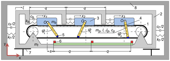
Figure 1. Physical model of the system. 1—conveyor belt, 2—housing, 3—bodies, 4—pendulum, 5—magnets, 6—coils, 7—rails, 8—frame.

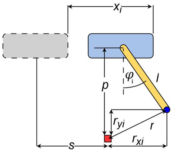
Figure 2. Distance between magnet and coil.

Starting the conveyor causes the upper branch of the belt to move in the X-direction at velocity v. As a result of friction between the bodies (3) and the conveyor belt, the system exhibits a dynamic response—its components begin to move. This response can be divided into two distinct phases: stick, during which a body does not move relative to the upper branch of the belt, and slip, during which the body moves relative to the upper branch of the belt. Let this motion be described by the following generalized coordinates: $x_i\left(t\right)= x_i$—the displacement of the $i$-th body relative to the housing, equivalent to the deflection of the spring $k_b$, ${\phi }_i\left(t\right)= {\phi }_i$—the angular displacement of the $i$-th pendulum relative to the vertical axis; $\xi \left(t\right)=\xi$—the displacement of the conveyor housing relative to the frame. The system thus has $2n+1=7$ degrees of freedom.

2.2. Mathematical Modeling

With $i=\mathrm{1,2},3,$ the equations of motion of the studied system in the slip phase can be derived using Lagrange’s equations of the second kind. The total kinetic energy $T$ of the system consists of the partial kinetic energies of the bodies $T_b$, the pendula $T_p$, and the frame $T_f$. These are given as follows:

$$T=T_b+T_p+T_f,$$

(1)

$$T_b={\displaystyle \frac{1}{2}}{m}_b{\sum }_{i=1}^3{\left(\dot{\xi }+{\dot{x}}_i\right)}^2,$$

(2)

$$T_p={\displaystyle \frac{1}{2}}{J}_c{{\dot{\phi }}_i}^2+{\displaystyle \frac{1}{2}} m_p\sum _{i=1}^3\left({\left(\xi +{\dot{x}}_i+{\displaystyle \frac{1}{2}}l \mathrm{c}\mathrm{o}\mathrm{s}\left({\phi }_i\right){\dot{\phi }}_i\right)}^2+{\left({\displaystyle \frac{1}{2}}l \mathrm{s}\mathrm{i}\mathrm{n}\left({\phi }_i\right){\dot{\phi }}_i\right)}^2\right),$$

(3)

$$T_f={\displaystyle \frac{1}{2}}{m}_f{\dot{\xi }}^2.$$

(4)

The total potential energy $V$ of the system consists of the potential energies of the body springs $V_b$, the pendula $V_p$, the housing springs $V_f$, and the energy of magnetic interaction between the coils and the magnets at the ends of the beams $V_e$, namely:

$$V=V_b+V_f+V_p+V_e,$$

(5)

$$V_b={\displaystyle \frac{1}{2}}{k}_b\sum _{i=1}^3{x_i}^2,$$

(6)

$$V_p={\displaystyle \frac{1}{2}}gl{m}_p\sum _{i=1}^3\left(1-\mathrm{c}\mathrm{o}\mathrm{s}\left({\phi }_i\right)\right),$$

(7)

$$V_f={\displaystyle \frac{1}{2}}{k}_f{\xi }^2.$$

(8)

The model of the electromagnetic interaction potential was adopted based on studies of pendula with magnetic interactions [4,5,6].

$$V_e=a\sum _{i=1}^3\exp \left({\displaystyle \frac{-{r_i}^2}{b}}\right).$$

(9)

It should be emphasized, however, that in the cited works the interaction energy was expressed as a function of the pendulum’s rotation angle. Here, a direct measure of the distance between the coil and the magnet—$r_i$—is used, as defined in Figure 2:

$$r_i=\sqrt{{r_{xi}}^2+{r_{yi}}^2},$$

(10)

where:

$$r_{xi}=l \mathrm{s}\mathrm{i}\mathrm{n}\left({\phi }_i\right)+x_i-s,$$

(11)

$$r_{yi}=p-l \mathrm{c}\mathrm{o}\mathrm{s}\left({\phi }_i\right).$$

(12)

The quantities $a$ [$\mathrm{N}\mathrm{m}$] and $b$ [${\mathrm{m}}^2$] are coefficients describing the maximum interaction energy and the rate of field decay, respectively. Their values can be determined experimentally.

The analyzed system is not idealized; therefore, energy dissipation $D$ also occurs. Dissipation takes place in the viscoelastic element connecting the body to the housing—$D_b$, in the viscoelastic element connecting the housing to the frame—$D_f$, and in the joint $O$ of the pendula—$D_p$. The components of the dissipation functions are as follows:

$$D=D_b+D_f+D_p,$$

(13)

$$D_b={\displaystyle \frac{1}{2}}{c}_b\sum _{i=1}^3{{\dot{x}}_i}^2,$$

(14)

$$D_p={\displaystyle \frac{1}{2}}{c}_p\sum _{i=1}^n{{\dot{\phi }}_i}^2,$$

(15)

$$D_f={\displaystyle \frac{1}{2}}{c}_f{\dot{\xi }}^2.$$

(16)

The system is subjected to friction forces between the bodies and the conveyor belt $F_i$. They take the general form:

$$F_i=f_i{P}_i.$$

(17)

The first coefficient in the above expression is the Stribeck friction model, given in the form:

$$f_i={\mu }_s\mathrm{t}\mathrm{a}\mathrm{n}\mathrm{h}\left({\displaystyle \frac{v-{\dot{x}}_i}{ϵ}}\right)-\alpha \left(v-{\dot{x}}_i\right)+\beta {\left(v-{\dot{x}}_i\right)}^3.$$

(18)

The coefficients ${\mu }_s$,$\alpha ,$ and $\beta$ are parameters characterizing the Stribeck friction curve and are determined experimentally for a given friction pair [15]. For a sufficiently small value of the parameter $ϵ\ll 1$, the $\mathrm{t}\mathrm{a}\mathrm{n}\mathrm{h}$ function is used as a continuous alternative to the discontinuous $\mathrm{s}\mathrm{i}\mathrm{g}\mathrm{n}$ function. An example of its behavior is shown in Figure 3.

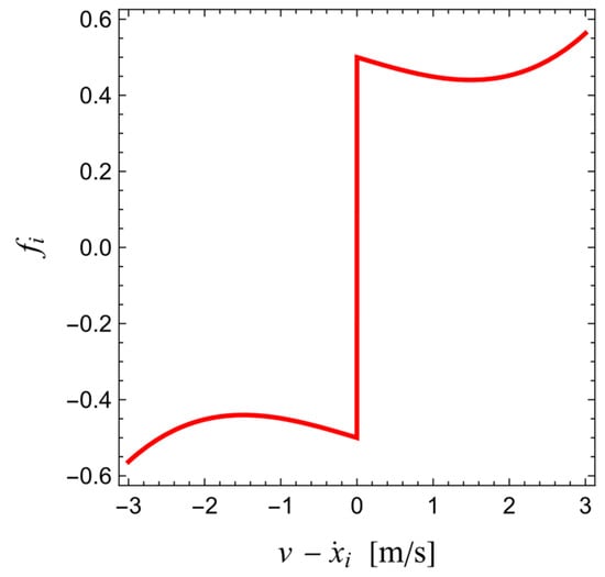
Figure 3. Exemplary Stribeck friction graph given by Equation (18) for ${\mu }_s=0.5, \alpha =0.060,\beta =0.009, \mathrm{a}\mathrm{n}\mathrm{d} ϵ=0.0001$.

The second term—$P_i$, is the force acting on the mass in the $Y$-direction. It is the sum of the gravitational force, the inertial force of the pendulum, the centrifugal force generated by it, and the vertical component of the magnetic interaction between the magnet and the coil:

$$P_i=-g\left(m_b+m_p\right)-{\displaystyle \frac{1}{2}}l{m}_p\left(\mathrm{s}\mathrm{i}\mathrm{n}\left({\phi }_i\right){\ddot{\phi }}_i+\mathrm{c}\mathrm{o}\mathrm{s}\left({\phi }_i\right){{\dot{\phi }}_i}^2\right)+\sum _{i=1}^3{E}_{yi},$$

(19)

where $E_{yi}$ is the $Y$-component of the magnetic interaction force between the magnet and the coil:

$$E_{yi}=2{\displaystyle \frac{a}{b}}\mathrm{e}\mathrm{x}\mathrm{p}\left(-{\displaystyle \frac{1}{b}}\left({\left(p-l \mathrm{c}\mathrm{o}\mathrm{s}\left({\phi }_i\right)\right)}^2+{\left(l \mathrm{s}\mathrm{i}\mathrm{n}\left({\phi }_i\right)+x_i-s\right)}^2\right)\right)\left(p-l \mathrm{c}\mathrm{o}\mathrm{s}\left({\phi }_i\right)\right).$$

(20)

Substituting the above expressions into Lagrange’s equation of the second kind results in the derivation of the equations of motion of the system in the slip phase. In the considered model, the belt velocity is $v=const.$; therefore, in the stick phase, the equation of motion of the body relative to the conveyor must take the following form:

$${\ddot{x}}_i=0.$$

(21)

The stick phase is observed as long as the velocity of the body is equal to the velocity of the belt, and the friction force ensures the static equilibrium of the body on the belt. Therefore, the following conditions must be satisfied:

$${\dot{x}}_i-v=0 \cap \left|H_i\right|\le \mu s P_i,$$

(22)

where:

$$H_i= -k{x}_i+E_{xi}-c{\dot{x}}_i+{\displaystyle \frac{1}{2}}l m_p\left(\mathrm{s}\mathrm{i}\mathrm{n}\left({\phi }_i\right){{\dot{\phi }}_i}^2-\mathrm{c}\mathrm{o}\mathrm{s}\left({\phi }_i\right){\ddot{\phi }}_i\right)-\left(m_b+m_p\right)\ddot{\xi },$$

(23)

$$E_{xi}={\displaystyle \frac{2a}{b}}\mathrm{e}\mathrm{x}\mathrm{p}\left({\displaystyle \frac{1}{b}}\left({\left(l \mathrm{c}\mathrm{o}\mathrm{s}\left({\phi }_i\right)-p\right)}^2+{\left(l \mathrm{s}\mathrm{i}\mathrm{n}\left({\phi }_i\right)+x_i-s\right)}^2\right)\right)\left(l \mathrm{s}\mathrm{i}\mathrm{n}\left({\phi }_i\right)+x_i-s\right)$$

(24)

The complete mathematical model of the studied system is therefore given by a system of equations:

$$\left(m_b+m_p\right){\ddot{x}}_i=\left\{\begin{array}{ccc}{H}_i-F_i& \mathrm{f}\mathrm{o}\mathrm{r}& \left|H_i\right|>\mu s{P}_i\\ 0& \mathrm{f}\mathrm{o}\mathrm{r}& {\dot{x}}_i-v=0\cap \left|H_i\right|\le \mu s{P}_i\end{array}\right.,$$

(25)

$$\left(J_c+{\displaystyle \frac{1}{4}}{l}^2 m_p\right){\ddot{\phi }}_i=-{\displaystyle \frac{\partial Ve}{\partial {\phi }_i}}-{\displaystyle \frac{1}{2}}gl m_{p}sin\left({\phi }_i\right)-c_p{\dot{\phi }}_i-{\displaystyle \frac{1}{2}}l m_{p}cos\left({\phi }_i\right)\left(\ddot{\xi }+{\ddot{x}}_i\right),$$

(26)

$$\left(3 m_b+m_f+3 m_p\right)\ddot{\xi }=-k_f\xi -c_f\dot{\xi }+\sum _{i=1}^3\left(H_i-\left(m_b+m_p\right){\dot{x}}_i\right),$$

(27)

or in dimensionless form:

$${\ddot{X}}_i=\left\{\begin{array}{ccc}\overline{H_i}-\overline{F_i}& \mathrm{f}\mathrm{o}\mathrm{r}& \left|\overline{H_i}\right|>\mu s\overline{P_i}\\ 0& \mathrm{f}\mathrm{o}\mathrm{r}& {\dot{X}}_i-\overline{v}=0\cap \left|\overline{H_i}\right|\le \mu s\overline{P_i}\end{array}\right.,$$

(28)

$$\begin{gathered} \overline{H_i}=-X_i-\overline{c_b}{\dot{X}}_i+{\displaystyle \frac{1}{2}}\overline{M_1}\overline{L_s}\left({\left({\dot{\Phi }}_i\right)}^2\sin \left({\Phi }_i\right)-{\ddot{\Phi }}_i\cos \left({\Phi }_i\right)\right)+ \\ 2\overline{a}\left(\overline{L_s}\sin \left({\Phi }_i\right)+X_i-1\right)\exp \begin{array}{c}\left(\overline{b_2}{\left(\overline{L_s}\sin \left({\Phi }_i\right)-X_i+1\right)}^2-\overline{b_1}{\left(1-\overline{L}\cos \left({\Phi }_i\right)\right)}^2\right)-\ddot{\Psi }\#\end{array} \end{gathered}$$

(29)

$$\begin{gathered} {\ddot{\Phi }}_i=2\kappa \overline{a}\overline{b_2}\overline{L_s}\left({\displaystyle \frac{\overline{L_s}}{\overline{L}}}\sin \left({\Phi }_i\right)-\left(1-X_i\right)\cos \left({\Phi }_i\right)\right) \\ \begin{array}{c}exp\left(\overline{b_2}{\left(\overline{L_s}\sin \left({\Phi }_i\right)-X_i+1\right)}^2+\overline{b_1}{\left(\overline{L}\cos \left({\Phi }_i\right)-1\right)}^2\right)\\ -\overline{c_p}{\dot{\Phi }}_i-{\displaystyle \frac{1}{2}}\overline{M_2}\cos \left({\Phi }_i\right)\left({\ddot{X}}_i+\ddot{\Psi }\right)-{\Omega }_2\sin \left({\Phi }_i\right),\end{array} \end{gathered}$$

(30)

$$\ddot{\Psi }=-\Psi {\Omega }_3-\dot{\Psi }\overline{c_b}+\sum _{i=1}^3{\displaystyle \frac{1}{2}}\gamma \overline{M_3}\overline{L_s}\left({\left({\dot{\Phi }}_i\right)}^2\sin \left({\Phi }_i\right)-{\ddot{\Phi }}_i\cos \left({\Phi }_i\right)\right)+\overline{M_3}\left(\gamma +1\right)\left(\overline{f_i}-{\ddot{X}}_i\right).$$

(31)

Functions $\overline{P_i}$, $\overline{f_i}$ and $\overline{F_i}$ are governed by the following expressions:

$$\overline{P_i}=2{\displaystyle \frac{\overline{L_s}}{\overline{L}}}\overline{a}\left(1-\overline{L}\cos \left({\Phi }_i\right)\right)\exp \left(-\overline{b_2}{\left(\overline{L_s}\sin \left({\Phi }_i\right)+X_i-1\right)}^2-\overline{b_1}{\left(1-\overline{L}\cos \left({\Phi }_i\right)\right)}^2\right)-\overline{g}-{\displaystyle \frac{1}{2}}\overline{M_1}\overline{L_s}\left({\left({\dot{\Phi }}_i\right)}^2\cos \left({\Phi }_i\right)+{\ddot{\Phi }}_i\sin \left({\Phi }_i\right)\right)$$

(32)

and dimensionless parameters are defined in the following way:

$$\begin{array}{c}{X}_i={\displaystyle \frac{x_i\left(\tau \right)}{s}},\Phi ={\phi }_i\left(\tau \right),\Psi ={\displaystyle \frac{\xi \left(\tau \right)}{s}},\tau =t{\omega }_1,\gamma ={\displaystyle \frac{m_b}{m_p}},\overline{b_1}={\displaystyle \frac{p^2}{b}},{{\omega }_1}^2={\displaystyle \frac{k_b}{m_b\left(1+\gamma \right)}},{{\omega }_2}^2={\displaystyle \frac{1}{2}}{\displaystyle \frac{gl\gamma m_b}{J_p+\frac{1}{4}{l}^2{m}_p}},\\ \overline{a}={\displaystyle \frac{a}{b{{\omega }_1}^2{m}_b\left(\gamma +1\right)}}, \overline{L}={\displaystyle \frac{l}{p}},\overline{b_2}={\displaystyle \frac{s^2}{b}},\overline{c_b}={\displaystyle \frac{c}{{\omega }_1{m}_b\left(\gamma +1\right)}},\overline{M_1}={\displaystyle \frac{\gamma }{\gamma +1}},\overline{v}={\displaystyle \frac{v}{s{\omega }_1}},\overline{\alpha }=\alpha s{\omega }_1,\overline{\beta }=\beta s^3{{\omega }_1}^3,\\ {\Omega }_2={\displaystyle \frac{{{\omega }_2}^2}{{{\omega }_1}^2}},{\Omega }_3={\displaystyle \frac{{{\omega }_3}^2}{{{\omega }_1}^2}},\overline{c_p}={\displaystyle \frac{c_p}{{\omega }_1\left(J_p+\frac{1}{4}\gamma l^2{m}_b\right)}},\overline{M_2}={\displaystyle \frac{\gamma \mathrm{l}{m}_b\mathrm{s}}{J_p+\frac{1}{4}\gamma l^2{m}_b}},\overline{c_b}={\displaystyle \frac{c_p}{{\omega }_1\left(m_{b}3\left(\gamma +1\right)+m_f\right)}},\\ \overline{M_3}={\displaystyle \frac{m_b}{m_{b}3\left(\gamma +1\right)+m_f}},\overline{g}={\displaystyle \frac{g}{s{{\omega }_1}^2}},\overline{ϵ}={\displaystyle \frac{ϵ}{s{\omega }_1}},\kappa ={\displaystyle \frac{J_p+\frac{1}{4}\gamma l^2{m}_b}{b\left(\gamma +1\right)m_b}}.\end{array}$$

(33)

3. The Influence of Magnetic Interaction

The analysis of the rich spectrum of dynamic phenomena occurring in the described system is conveniently conducted using bifurcation diagrams of the individual generalized coordinates. Due to the asymmetry of stick–slip oscillations, both extrema of the amplitude–time response—namely maxima $d_{max}$ and minima $d_{min}$—are shown on the bifurcation diagram. Here, the amplitude $∆d$ is defined as the difference between the maximum and minimum displacement (see Figure 4).

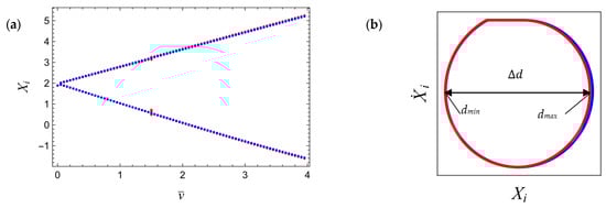
Figure 4. Bifurcation diagram (a) and phase portrait (b) of $X_i$ coordinate for $\overline{a}=0.03$ (red dots) and $\overline{a}=0$ (blue dots).

Such diagrams allow observation of the evolution of oscillation amplitudes for individual degrees of freedom as a result of increasing the belt velocity from zero. The belt velocity was incremented in steps of 0.05 velocity units $\overline{v}$. To eliminate the influence of transient processes on the obtained results, amplitudes were recorded after 50,000 units of dimensionless time $\tau$, over a period of 500 $\tau$ units. Numerical computations were carried out in the Wolfram Mathematica 14.2 environment. The discontinuous transitions between sticking and slipping were implemented using the WhenEvent construct with “RestartIntegration” and “StepBegin” options, ensuring that the integration restarts locally whenever a contact regime changes. This approach allows the solver to capture instantaneous changes in velocity or force without introducing unphysical oscillations or numerical artifacts. The computations employed the IDA solver based on the implicit BDF method for differential-algebraic systems, with equation simplification performed through residual analysis and the maximum differentiation order limited to three.

Let us now examine the influence of the magnetic interaction force on the system’s behavior, assuming that the mass of the pendulum is small in relation to the mass of the body, i.e., $\gamma =0.1$. To this end, bifurcation diagrams and phase portraits of the coordinates $X_i$ (Figure 4), $\Psi$ (Figure 5), and ${\Phi }_i$(Figure 6) are presented for two variants of the system parameters: one with $\overline{a}=0.03$ (red) and the other with $\overline{a}=0$ (blue). The remaining parameter values are as follows:

$$\begin{gathered} \overline{L_s}=7.42,\overline{b_1}=48.0,\overline{L}=0.98,\overline{b_2}=0.65,\overline{c_1}=0.0067, \\ \overline{v}=2.6876,\overline{\alpha }=0.011,\overline{\beta }=0.0000579,\overline{g}=3.968,{\Omega }_2=0.4, \\ \overline{c_p}=0.01,{\Omega }_3=0.106,\overline{c_b}=0.043,\overline{M_2}=0.2, \\ \overline{M_4}=0.08, {\mu }_s=0.5,\gamma =0.1,\kappa =2.50,\overline{ϵ}=0.00053. \end{gathered}$$

(34)

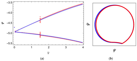
Figure 5. Bifurcation diagram (a) and phase portrait (b) of $\Psi$ coordinate for $\overline{a}=0.03$ (red) and $\overline{a}=0$ (blue).

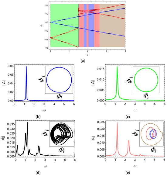
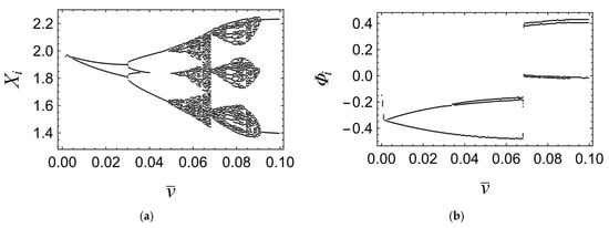
Figure 6. Bifurcation diagram (a) of ${\Phi }_i,$ coordinate for $\overline{a}=0.03$ (red dots) and $\overline{a}=0$ (blue dots). Phase portraits and corresponding frequency spectra below: (b) for the system with $\overline{a}=0,$ (c–e)—for the system with $\overline{a}=0.03$. Color of the phase portrait corresponds to the belt velocity $\overline{v}$ range marked on the bifurcation diagram.

All initial conditions rest to zero, i.e., we have:

$$\begin{gathered} X_1\left(0\right)=X_2\left(0\right)=X_3=\left(0\right)={\Phi }_1\left(0\right)={\Phi }_2\left(0\right)={\Phi }_3\left(0\right)=\Psi \left(0\right)= \\ {\dot{X}}_1\left(0\right)={\dot{X}}_2\left(0\right)={\dot{X}}_3\left(0\right)={\dot{\Phi }}_1\left(0\right)={\dot{\Phi }}_2\left(0\right)={\dot{\Phi }}_3\left(0\right)=\dot{\Psi }\left(0\right)=0 \end{gathered}$$

(35)

Given that the initial conditions of all subsystems are identical, it is to be expected that $X_1=X_2=X_3$ and ${\Phi }_1={\Phi }_2={\Phi }_3$. In this part of the study, we will therefore use the general notation $X_i$ and ${\Phi }_i$ accordingly.

The presented maps indicate that the magnetic interaction of the specified magnitude exerts a marginal influence on the oscillations of the bodies on the belt as well as on the vibrations of the frame and frequencies of the system. However, its qualitative impact on the pendulum position is evident—for low belt velocities, the pendulum, repelled by the coil, oscillates around negative positions (green domain). An increase in belt velocity leads to an increase in the amplitude of body vibrations, and with a sufficiently large deflection, the pendulum jumps to the other side of the magnetic field—a saddle-node bifurcation occurs, thereby changing the position about which it oscillates for velocities $\overline{v}>1.502$. It should be noted that this transition is accompanied by irregular oscillations observable in all coordinates (black domain), but ultimately a limit cycle is formed, whose character alternates with increasing velocity (red and blue domain), eventually leading to uniform oscillations (brown domain). It is also worth noting that in all ranges, except for the irregular (black) one, the main frequencies remain identical and equal to ${\omega }_m = 1.13$. This indicates that the oscillations of the system remain unsynchronized only in the neighborhood of the saddle-node bifurcation velocity. This conclusion is also supported by the Lissajous diagrams shown in Figure 7.

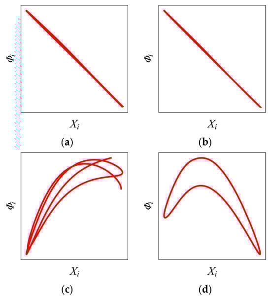
Figure 7. Lissajous diagrams showing synchronization of $X_i$ and ${\Phi }_i$ for different belt velocities. (a) $\overline{v}=0.15$, (b) $\overline{v}=1.11$, (c) $\overline{v}=1.51$, (d) $\overline{v}=2.25$.

It is also important to note that in the case of the system subject to magnetic interaction, the amplitude of pendulum oscillations is non-monotonic with respect to belt velocity—in the case of $\overline{a}=0.03$, a distinct decrease in amplitude is observed in blue and red regions, which suggests that the pendulum experiences levitation within the magnetic field and remains close to static equilibrium. The effect of increasing the magnetic interaction parameter $\overline{a}$ on the extent of this phenomenon is conveniently visualized using a two-dimensional map (Figure 8), where the horizontal axis represents the belt velocity $\overline{v}$, the vertical axis denotes the value of $\overline{a}$, and the difference between the maximum and minimum displacement is represented by the corresponding color. The map also indicates the parameter regions corresponding to specific types of solutions—single-period (1T), period-doubled (2T), and chaotic (C) behavior.

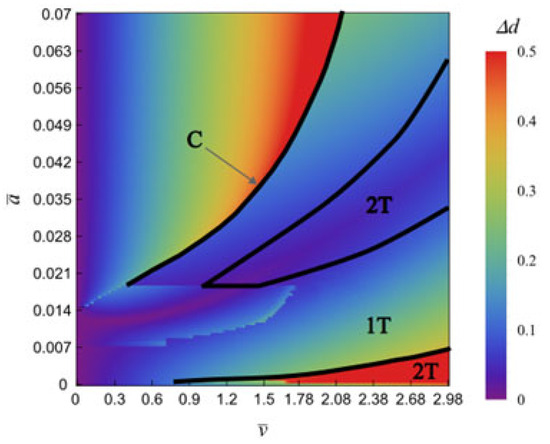
Figure 8. Two-dimensional bifurcation diagram of ${\Phi }_i$ coordinate. Black lines delimit areas with specific types of solutions: 1T—single-period, 2T—period-doubled, C—chaos.

The figure clearly shows a tongue of low amplitudes stretching across the map. This indicates that the amplitude minimum is reached at progressively higher belt velocities as the magnetic interaction parameter $\overline{a}$ increases. Moreover, the value of this minimum grows with increasing belt velocity.

The map also reveals two additional phenomena that were not visible in the previously presented bifurcation diagrams. For small values of $\overline{a}$, a sudden increase in the amplitude of pendulum oscillations is observed at a certain belt velocity. This corresponds to a period-doubling of the orbit (Figure 9), for a set of parameters for which the pendulum enters the bifurcation scenario “behind” the coil. The map (Figure 8) also displays a tongue of elevated amplitudes that penetrates the diagram as a horizontal band for $0.0076<\overline{a}<0.1821$ and belt velocities not exceeding $1.73$. Within this region, a local minimum in pendulum oscillation amplitude can be observed, but it occurs prior to the bifurcation of the limit cycle (Figure 10).

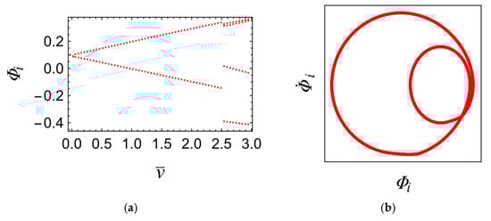
Figure 9. Bifurcation diagram of ${\Phi }_i$ coordinate for $\overline{a}=0.005$ (a) and the corresponding phase portrait for $\overline{v}=2.38$ (b).

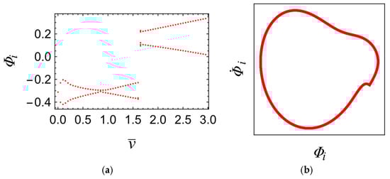
Figure 10. Bifurcation diagram of ${\Phi }_i$ coordinate for $\overline{a}=0.015$ (a) and the corresponding phase portrait for $\overline{v}=0.58$ (b).

The analysis of the map presented in Figure 8 thus leads to the conclusion that, by means of the magnetic interaction force, it is possible to control not only the equilibrium position of the pendula but also the amplitude of their oscillations—up to an almost complete suppression of these oscillations. It should be emphasized, however, that no significant qualitative or quantitative influence of the pendula behavior on the behavior of the remaining elements of the system has been demonstrated. Therefore, it cannot be stated that the coil–pendulum–body interaction enables control of stick–slip oscillations, at least within the system characterized by the parameters specified in (33) and (34). Such a pendulum may serve as an analog carrier of information about the body’s limit cycle—a qualitative change in the pendulum’s behavior or its synchronization with another pendulum may convey information that the body has exceeded a certain vibration amplitude [6,7], while the moment of detection can be adjusted through the magnetic interaction force.

4. Effect of Initial Conditions

The investigated system consists, among other components, of three identical oscillators connected via joints to pendula. Until now, the initial conditions of these subsystems have been identical, and thus, no differences in their behavior could be observed. Let us now examine the system with the same set of parameters (34), but with different initial conditions, namely:

$$\begin{gathered} X_1\left(0\right)=2 \\ \begin{array}{c}{X}_2\left(0\right)=X_3=\left(0\right)={\Phi }_1\left(0\right)={\Phi }_2\left(0\right)={\Phi }_3\left(0\right)=\Psi \left(0\right)={\dot{X}}_1\left(0\right)=\\ {\dot{X}}_2\left(0\right)={\dot{X}}_3\left(0\right)={\dot{\Phi }}_1\left(0\right)={\dot{\Phi }}_2\left(0\right)={\dot{\Phi }}_3\left(0\right)=\dot{\Psi }\left(0\right)=0\end{array} \end{gathered}$$

(36)

Such a set of initial conditions justifies the assumption that $X_2=X_3=X_j$ and ${\Phi }_2={\Phi }_3={\Phi }_j$. The bifurcation diagrams in Figure 11 compare systems with initial conditions (35) (blue) and (36) (red).

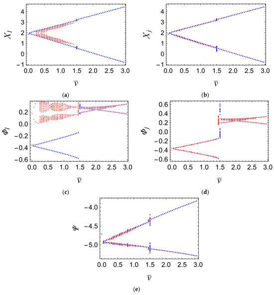
Figure 11. Bifurcation diagrams for $X_1\left(0\right)=2$ (red) and $X_1\left(0\right)=0$ (blue) of coordinates: (a) $X_1$, (b) $X_j$, (c) ${\Phi }_1$, (d) ${\Phi }_j$, (e) $\Psi$.

Although the influence of the change in initial condition is noticeable in each of the generalized coordinates, it is naturally most pronounced in the first subsystem, whose initial condition was altered. A qualitative change is particularly evident in the angular displacement ${\Phi }_1$—the pendulum of the first subsystem oscillates around a positive position, exhibiting qualitatively different behavior. For belt velocities $\overline{v}<0.32$, the pendulum reaches a limit cycle (Figure 12), whereas upon exceeding this velocity, a subcritical Neimark–Sacker bifurcation occurs, followed by the emergence of quasiperiodic oscillations (Figure 13). It is worth noting that the amplitude of these oscillations decreases with increasing belt velocity until the remaining two pendula undergo a saddle-node bifurcation. It should be emphasized that the belt velocity at which this transition occurs is lower than in the previously studied case for $X_1\left(0\right)=0.$

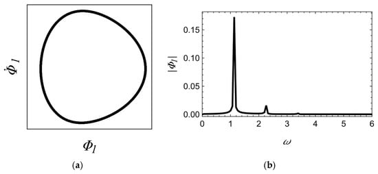
Figure 12. Phase portrait (a) and frequency spectrum (b) of ${\Phi }_1$ corresponding to the bifurcation map, Figure 11c at $\overline{v}=0.15$.

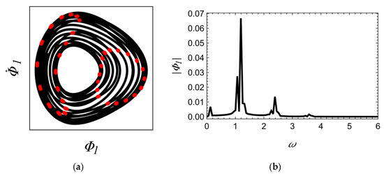
Figure 13. Phase portrait of ${\Phi }_1$ (a) and frequency spectrum (b) corresponding to the bifurcation map, Figure 11c at $\overline{v}=0.15$. Red dots create a Poincaré section. Sampling moments were determined as the times at which ${\dot{X}}_1=0$.

It is therefore justified to conclude that the behavior of the pendulum may also serve as an indicator of the initial condition imposed on the body to which the pendulum is attached. The pendulum may oscillate “in front of” or “behind” the coil, depending on the initial condition specified for the body to which it is fixed. According to the conclusions drawn in the previous chapter, the position of the mass at which the pendulum transitions between these two configurations can be adjusted by varying the intensity of the magnetic interaction. It should be noted that inducing oscillations of the pendulum “behind” the coil at low belt velocities, by prescribing an appropriate initial condition of the body, leads to the onset of quasiperiodic oscillations—whereas when such a state is induced by tuning the magnetic interaction force (Figure 9), this effect does not occur. This phenomenon can therefore be regarded, on the one hand, as an additional diagnostic indicator, and on the other, as an undesirable effect resulting in an unacceptable interference with the behavior of the primary system.

Notably, within the belt velocity range in which the pendulum of the first subsystem exhibits regular oscillations ($\overline{v}<0.32$), $X_1$ remains synchronized with ${\Phi }_1$, whereas $X_j$ and ${\Phi }_j$ move asynchronously. In the quasiperiodic oscillation region ($0.32<\overline{v}<1.49$), this pattern is reversed—$X_j$ and ${\Phi }_j$ are synchronized, while $X_1$ and ${\Phi }_1$ are not.

Synchronization also occurs between the responses $X_1$ and $X_j$ at belt velocity $0.32<\overline{v}<1.49$. Moreover, full system synchronization takes place in the post saddle-node bifurcation region. Consequently, it can be concluded that the analysis of synchronization among individual segments of the system may provide valuable insights not only into the initial conditions but also into the belt velocity, which is strongly correlated with the vibration amplitudes of the bodies. The discussed sequence of phenomena is illustrated by the Lissajous figures shown in Figure 14.

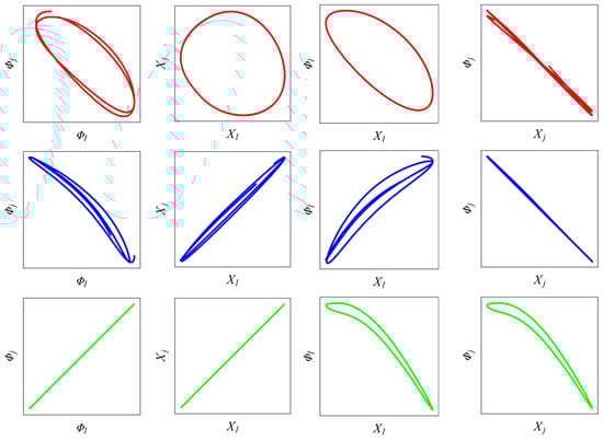
Figure 14. Lissajous diagrams corresponding to bifurcation maps in Figure 11. Colors distinguish different belt velocities: red—$\overline{v}=0.15$, blue—$\overline{v}=1.11$, green—$\overline{v}=1.51$.

A natural extension of such analysis is to investigate the influence of a wide range of initial conditions $X_1\left(0\right)$ and ${\dot{X}}_2\left(0\right)$ on the system’s behavior. However, exploration of the initial condition space did not reveal any set of conditions that would lead to qualitatively different behavior than those discussed so far—manipulation of the initial position and velocity of the body affects only the attractor to which the pendulum is drawn at low belt velocity. This attractor may correspond to positions “in front of” or “behind” the coil. Both motion variants are illustrated in Figure 11c, marked in blue and red, respectively.

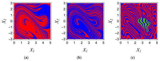
It should be noted, however, that the system is sensitive to initial conditions. An example of the basin of attraction in $X_1- {\dot{X}}_1$ space is shown in Figure 15. The fractal structure of the basin of attraction partially limits the ability to diagnose the body’s initial condition based on the range of pendulum oscillations, as it indicates the unpredictability of the equilibrium position to which the pendulum will be drawn. However, it should be noted that the fractal structure of these basins is observed mostly when approximately $\left|{\dot{X}}_1\right|<1$; therefore, for small initial velocities of the body, it is possible to predict the equilibrium position around which the pendulum will oscillate.

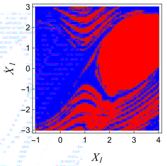
Figure 15. Basin of attraction of ${\Phi }_1$ in $X_1- {\dot{X}}_1$ space and with the remaining boundary conditions set to 0. Blue—in front of the coil, red—behind the coil.

An additional variation in one of the initial conditions of the remaining masses, e.g., $X_2\left(0\right)$, affects to some extent the attraction of the pendulum toward a given equilibrium position (Figure 16), but this change is sufficiently small that there is no basis to conclude that the pendulum’s behavior can also be used to diagnose the initial condition imposed on a body not directly coupled with the observed pendulum.

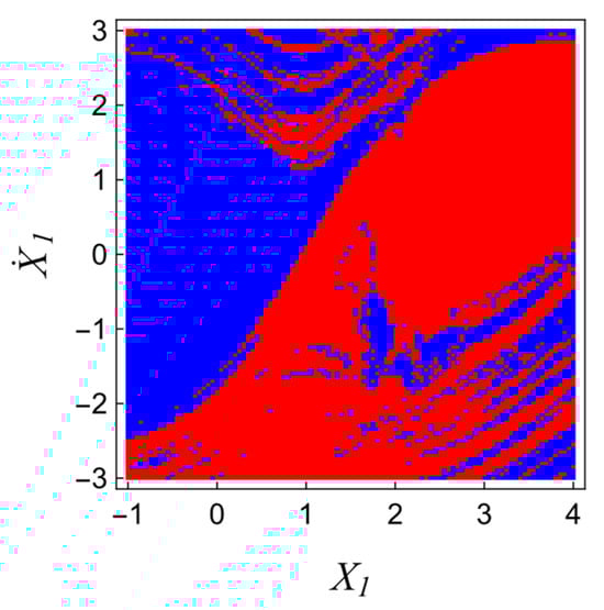
Figure 16. Basin of attraction of ${\Phi }_1$ in $X_1- {\dot{X}}_1$ space with $X_2\left(0\right)=2$ and the remaining boundary conditions set to 0. Blue—in front of the coil, red—behind the coil.

Thus far, it has been demonstrated that by manipulating the initial conditions of the bodies, one can induce one of two bifurcation patterns of the pendula. In the first pattern, the pendulum oscillates “in front of” the coil at low belt velocities and subsequently bifurcates “behind” it, whereas in the alternative bifurcation scenario, the pendulum remains “behind” the coil throughout the entire range of belt velocities. However, by altering the initial conditions of individual pendula, it is possible to induce alternative scenarios of amplitude variation of pendulum oscillations with changing belt velocity. Through manipulation of the initial conditions ${\Phi }_1\left(0\right)$ and ${\dot{\Phi }}_1\left(0\right)$, six distinct bifurcation maps describing the evolution of pendulum oscillation amplitudes were identified. These are presented in Figure 17.

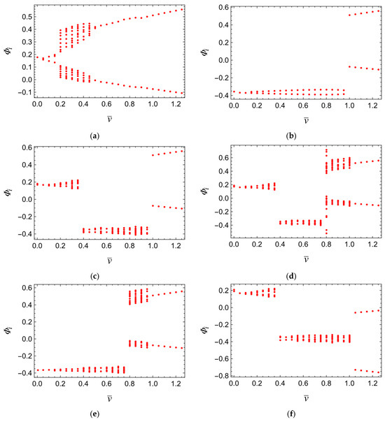
Figure 17. Identified bifurcation patterns.

The presented bifurcation maps indicate that the bifurcation scenarios of the pendula are not determined solely by the oscillation position relative to the coil at low belt velocities. After assuming the initial position, the pendulum may transition to the opposite side of the coil at different belt velocities or may not undergo such a transition at all. This phenomenon is well illustrated by the comparison of scenarios (c) and (f). Up to the belt velocity $v \approx 0.95$, both exhibit qualitatively similar quasiperiodic oscillations. Above this velocity, a reverse Neimark–Sacker bifurcation occurs, leading to the appearance of 1T oscillations, with the distinction that in scenario (c) this transition is accompanied by a jump “behind” the coil, whereas in scenario (f) the pendulum remains “in front of” the coil. This behavior demonstrates the system’s significant sensitivity, as even a small quantitative change in the system’s state—typical for quasiperiodic oscillations—may determine whether or not a bifurcation takes place.

The multitude of bifurcation patterns that the system can exhibit opens up the possibility for each subsystem to display different behavior during the operation of the conveyor. This is indeed the case, as illustrated by the distinct basins of attraction for each pendulum, shown in Figure 18.

Figure 18. Attraction maps to bifurcation patterns shown in Figure 17: (a) ${\Phi }_1$, (b) ${\Phi }_2$, (c) ${\Phi }_3$. Blue—(Figure 17a), Red—(Figure 17b), Green—(Figure 17c), Yellow—(Figure 17d), White—(Figure 17e), Black—(Figure 17f).

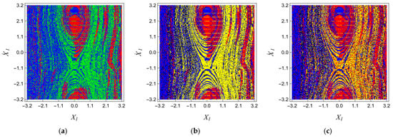
The complex, irregular structure of the maps illustrates the relationship between the initial conditions $X_1-{\dot{X}}_1$ and the bifurcation scenario of individual pendula indicates a strong sensitivity of the system to its initial conditions. This fact, combined with the previously discussed instability of each bifurcation scenario, leads to the conclusion that assigning nonzero initial conditions to the generalized coordinates describing the pendula results in significant unpredictability of their behavior. Similar results have been presented in [6,15,19]. Such a property of the system complicates its control through parameter adjustment. On the other hand, the multitude of possible states attainable by the system, when combined with external control ensuring stabilization [18,19], may provide the versatility desired in systems designed for energy recovery or vibration damping [10,11,12,13,14].

5. The Effect of Pendula Inertia Parameters

It should be emphasized at the outset that the analyses presented in the earlier sections of this study were carried out under the assumption that the pendulum mass was relatively small when compared to the total mass of the body ($\gamma =0.1$). This assumption, corresponding to the parameter configuration reported in dataset (34), implied that the oscillatory contribution of the pendulum could be treated essentially as a weak perturbation of the body’s overall motion. In practical terms, the trajectories of the body on the conveyor belt, as well as the oscillatory response of the supporting frame, were only marginally affected by the pendulum’s swinging motion. The body and the frame have therefore exhibited relatively simple dynamical patterns, which, while already non-trivial, did not capture the full richness of nonlinear phenomena possible in such a coupled mechanical arrangement.

In the present section, we abandon this restrictive assumption and consider instead the case where the ratio of the pendulum mass to the body mass is substantially larger, namely, $\gamma =0.5$. Additionally, the magnetic force multiplayer $\overline{\alpha }$ has been set to $\overline{\alpha }=0.02$. The rest of the values of the system parameters, together with the set of initial conditions employed, remained as provided in Equations (34) and (35). This change has profound dynamical consequences: it enhances the degree of coupling between the pendulum and the translational motion of the body, and as a direct result, the pendulum oscillations exert a much more pronounced influence on the global behavior of the system. Under these conditions, a considerably more intricate bifurcation structure emerges, and the system becomes capable of displaying a wide spectrum of nonlinear responses, ranging from regular single-period, multi-period motion, through to quasiperiodic oscillations.

To systematically illustrate these new dynamical regimes, bifurcation diagrams corresponding to the individual generalized coordinates of the system are presented in Figure 19. These diagrams provide an overview of how the qualitative nature of the attractors evolves as the control parameter, namely the belt velocity $\overline{v}$, is gradually increased. In addition, to enable a clearer resolution of the fine details of the transitions, magnified views of selected portions of the bifurcation are displayed in Figure 20.

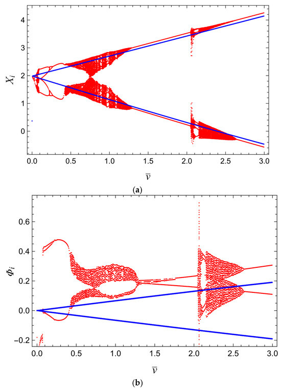
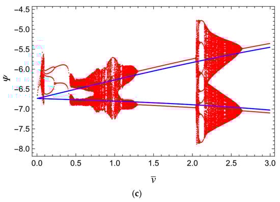
Figure 19. Bifurcation diagrams of (a) $X_i$, (b) ${\Phi }_i$, (c) $\Psi$. Blue—$\overline{\alpha }=0.02$, red—$\overline{\alpha }=0$.

Figure 20. Enlarged view of (a) Figure 19a, (b) Figure 19b.

These enlarged representations allow for a precise identification of critical thresholds, subtle stability changes, and the emergence of new oscillatory modes that are less apparent in the global diagrams. A qualitative change in the system’s behavior becomes evident even at relatively low belt velocities when the pendulum mass is increased. For values of $\overline{v}\le 0.0295$, the system exhibits a single-loop periodic trajectory. This orbit with frequency ${\omega }_m\approx 1.32$ originates from a grazing–sliding bifurcation, as depicted in Figure 21a. In the spectrum, we can also observe an incommensurate frequency ${\omega }_n=3.89$ of small amplitude, which indicates that the system exhibits nearly periodic oscillations. As the belt velocity is further increased $\overline{v}=0.0301$, the single-period solution loses stability through a period-doubling bifurcation. Beyond this point, the system develops a trajectory of the splitting–merging type [19], characterized by the emergence of a subharmonic loop with doubled period (see Figure 21b). In the spectrum, we can now observe harmonic frequencies at ${\omega }_s= 0.65$. Given that ${\omega }_n/{\omega }_s \approx 6$, the subharmonic loop synchronizes the previously incommensurate frequency, and the system thus exhibits periodic behavior.

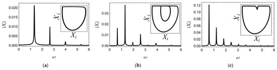
Figure 21. Phase portraits and corresponding frequency spectra of $X_i$ coordinate for (a) $\overline{v}=0.0295$, (b) $\overline{v}=0.0351$, (c) $\overline{v}=0.0455$.

With further growth of the control parameter, the subharmonic loop evolves in such a way that its period effectively decreases. Eventually, at a velocity of $\overline{v}=0.0405$, the loop collapses, which in the phase space corresponds to the division of the sliding surface, as illustrated in Figure 21c. This division persists to $\overline{v}=0.0501$ until the corresponding orbit ultimately loses stability. The destabilization occurs via a supercritical Neimark–Sacker bifurcation, beyond which the dynamics no longer remain confined to a single closed loop. Instead, an invariant complex torus is created, leading to quasiperiodic oscillations. It should be noted that the stroboscopic points on the Poincaré section form a very complex closed structure, but the trajectories do not indicate any symptoms of a chaotic attractor (Figure 22a). At higher velocities, an additional qualitative change occurs in the pendulum’s motion. At $\overline{v}=0.06515,$ a saddle-node bifurcation is triggered when the pendulum begins to oscillate on the opposite side of the coil. This transition is captured clearly in the bifurcation diagram of the ${\phi }_i$ coordinate presented in Figure 20b. After this jump, the body continues to display quasiperiodic motion; however, these oscillations are now clearly attracted by a nearby subharmonic orbit (Figure 22b). It should be noted that the complex structure of the curves visible in the Poincaré section indicates the complexity of the phase space of these trajectories.

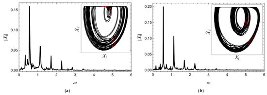
Figure 22. Phase portraits and corresponding frequency spectra of $X_i$ coordinate for (a) $\overline{v}=0.06301$, (b) $\overline{v}=0.08551$. Red dots create a Poincaré section whose sampling moments were determined as the times at which $\dot{\Psi }=0$.

Further along the parameter axis, at belt velocity $\overline{v}=0.0915,$ the system undergoes another significant transition. The quasiperiodic motion gives way to a single-period orbit, analogous to the one presented in Figure 21c, emerging through a subcritical Neimark–Sacker bifurcation. This event marks the restoration of periodic motion. At this stage, the pendulum is observed to cross the zero position during its oscillations, which indicates that the motion has re-entered an intrawell regime. As illustrated in Figure 19a, up to $\overline{v}=0.4331$, the body displays both 1T and 2T oscillations. These periodic responses are indicative of synchronized or mode-locked states between the pendulum and the translational motion of the body. Beyond the belt velocity $\overline{v}=0.4332$, when the pendulum exhibits interwell oscillations, we again observe quasiperiodic motion of the body and a sequence of both supercritical and subcritical Neimark–Sacker bifurcations. Similar sequences have also been observed in [15,19]. The bifurcation map (Figure 23) may suggest the emergence of periodic windows; however, spectral analysis indicates that what actually occurs is a sequence of increases and decreases in the torus dimension—the number of incommensurate frequencies in the spectrum is changing, but at least two presets remain (Figure 24). The system, therefore, remains unsynchronized. Such behavior persists until $\overline{v}=1.3416$ when the pendulum ultimately achieves a quasi-levitation state within the coil’s magnetic field, as discussed previously in Section 3. Up to $\overline{v}=2.0036$, the pendulum executes small-amplitude oscillations that exert minimal perturbation on the body and the frame.

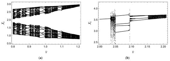
Figure 23. Enlarged view of Figure 19a for: (a) $\overline{v}\in \left(0.8, 1.2\right),\left(\mathbf{b}\right)\overline{v}\in (2.0, 2.2)$.

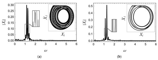
Figure 24. Phase portraits of $X_i$ coordinate for (a) $\overline{v}=0.8001$, (b) $\overline{v}=0.9151$.

Consequently, the body’s motion is simplified to 1T periodic orbits. However, once the belt velocity surpasses this range, Neimark–Sacker bifurcation is encountered, followed by torus breakdown, which again introduces quasiperiodic oscillations into the system’s dynamics, riffled with manifolds with almost-periodic 4T orbits (Figure 23 and Figure 25). Such behavior remains until $\overline{v}=2.6531$. Above that belt velocity, the system continues following a simple, almost-periodic 1T orbit.

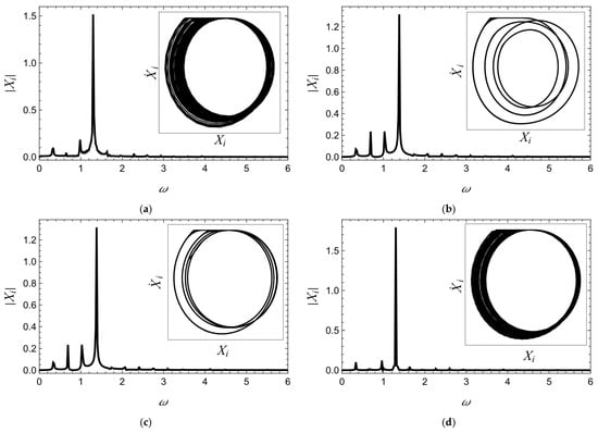
Figure 25. Phase portraits and corresponding frequency spectra of $X_i$ coordinate for (a) $\overline{v}=2.0361$, (b) $\overline{v}=2.0521$, (c) $\overline{v}=2.1191$, (d) $\overline{v}=2.2061$.

In the case of a pendulum system with large relative masses, numerous bifurcations are observed as the belt velocity increases. These bifurcations are not solely the result of changes in the equilibrium positions around which the pendulum oscillates—bifurcations also occur when the pendulum maintains the same oscillation position. It should be emphasized that such behavior arises exclusively from the variation of the pendulum’s inertial parameters. If the coil’s interaction with the body through the pendulum, via a normal force affecting the friction between the body and the belt, played a significant role, the magnetic interaction magnitude would have a greater influence on the body’s behavior in the cases discussed in Section 3 and Section 4, where $\gamma = 0.1$.

Within the analyzed range of belt velocities, the system exhibits both periodic and quasiperiodic oscillations of varying complexity. As illustrated in Figure 26, the belt velocities at which specific types of attractors emerge can be influenced by adjusting the electromagnetic interaction coefficient $\mathrm{a}$. Therefore, the system can be tuned to exhibit quasiperiodic oscillations at a selected belt velocity and subsequently stabilized, through appropriate control [20,21], to achieve the desired modal characteristics at that velocity. The ability to perform such operations is highly desirable in the design of vibration absorber systems [10,11], as well as in energy harvesting systems [12,13,14].

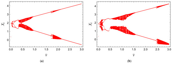
Figure 26. The influence of the magnetic interaction force coefficient a on the bifurcation scenario: (a $)\overline{a}=0.15,$ (b) $\overline{a}=0.25$.

The system, therefore, demonstrates highly intricate dynamical behavior. Moreover, depending on the choice of initial conditions, the evolution of the system as the belt velocity is varied may be represented by different bifurcation patterns—in the explored space: $X_i\in \left[-1, 4\right],{\dot{X}}_i\in \left[-3, 3\right], {\Phi }_i\in \left[-\pi ; \pi \right], {\dot{\Phi }}_i \in \left[-\pi , \pi \right],\Psi \in \left[-3, 3\right]$,$\dot{\Psi }\in \left[-3, 3\right],$ two alternative bifurcation patterns were identified. One of them corresponds to the case in which the pendulum oscillates “in front of” the coil throughout the entire range of belt velocities. When the system is initialized in this alternative configuration, the body’s motion at low velocities, specifically for $\overline{v}<0.4332$ is characterized by a simple single-periodic orbit. As the velocity surpasses this threshold, the system undergoes a Neimark–Sacker bifurcation, beyond which the qualitative behavior closely resembles that of the previously analyzed scenario (Figure 27).

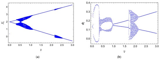
Figure 27. Bifurcation diagram—second variant. (a) $X_i$ coordinate, (b) ${\Phi }_i$ coordinate.

A distinctive feature of the third bifurcation pattern is that, in this case, for belt velocities $v¯ < 0.06515$, the pendulum does not oscillate but rotates—there is no amplitude record in the given range on the bifurcation diagram. After exceeding this velocity, the system bifurcates into behavior qualitatively identical to that described above. It should be emphasized that, whether the pendulum oscillates “behind” the coil or rotates at low belt velocities, the body’s behavior remains qualitatively the same (Figure 28).

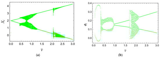
Figure 28. Bifurcation diagram—third variant. (a) $X_i$ coordinate, (b) ${\Phi }_i$ coordinate.

The relationship between the initial conditions and the bifurcation pattern of the system as the belt velocity varies is most conveniently characterized using basins of attraction. Figure 29 presents maps that assign a specific set of initial conditions on the $X_1 - X_2$ plane to the corresponding bifurcation pattern exhibited by each of the three subsystems. The values of the remaining initial conditions, which do not constitute the domain of the basins, were chosen arbitrarily. These are $X_3\left(0\right)=1.11,{\dot{X}}_3\left(0\right)=-0.58, {\mathsf{\Phi }}_3\left(0\right)=-0.72, {\dot{X}}_1\left(0\right)={\dot{X}}_2\left(0\right)={\mathsf{\Phi }}_1\left(0\right)={\dot{\mathsf{\Phi }}}_1\left(0\right)={\mathsf{\Phi }}_2\left(0\right)={\dot{\mathsf{\Phi }}}_2\left(0\right)={\dot{\mathsf{\Phi }}}_3\left(0\right)=\mathsf{\Psi }\left(0\right)=\dot{\mathsf{\Psi }}\left(0\right)=0$.

Figure 29. Maps of attraction to bifurcation patterns. Subsystems: (a) $1$, (b) $2$, (c) $3$. Red—(Figure 19a), Blue—(Figure 27), Green—(Figure 28).

As shown in Figure 29, the basins of attraction associated with subsystems 1 and 2—that is, the two elements whose initial conditions are being varied—exhibit qualitatively similar features. Their boundaries are relatively regular, in contrast to analogous diagrams mapping the bifurcation courses of a system with light pendula (Figure 18). Nonetheless, the basin of attraction corresponding to the third subsystem differs qualitatively from the former two. It lacks the same degree of regularity, but more importantly, we can observe a small but clearly identifiable region of attraction in the third scenario. The basins also indicate that by appropriately selecting the boundary conditions, it is possible to induce qualitatively different behavior in each of the three subsystems, at least for belt velocities sufficiently low for the differences between scenarios 2 and 3 to be observable.

Although the system with heavy pendula proves to be multistable and sensitive to initial conditions, it should be emphasized that the differences between the presented bifurcation patterns are limited to low belt velocities. This implies that, in a broader sense, the system maintains a high degree of predictability.

6. Summary

The analyzed system exhibits a rich dynamical landscape. Numerical analysis identified saddle-node, Neimark–Sacker, period-doubling, and other bifurcations, yielding multiple coexisting periodic, quasiperiodic, and chaotic attractors. Bifurcation diagrams illustrated how these attractors evolve with belt speed: at low speeds, the system settles into low-amplitude periodic motion, then undergoes bifurcations as speed increases. Such observation is consistent with earlier friction–pendulum and drill-string models [15,19], which reported similar irregular multi-period stick–slip responses. We also observed that the basins of attraction are highly fractal, indicating extreme sensitivity to initial conditions, typical for stick–slip systems [3,16] and axially moving masses in general [28,29,30].

The magnetic coupling strongly influenced synchronization. With pendula of small mass ratio, each pendulum readily phase-locks to the body motion, producing simple 1:1 or 1:2 mode-locked oscillations in each body–pendulum pair. This frequency entrainment result parallels previously studied forced and autonomous stick–slip systems [15,19]. In contrast, pendula of greater mass ratio become significant drivers and do not allow synchronization. Instead, the system develops a quasiperiodic attractor and undergoes sequences of bifurcations as belt velocity increases. Heavier pendula thus resist synchronization and effectively break the simple lock-in. It should be noted that partial synchronization has been observed: in some velocity ranges, the system demonstrated almost-periodic oscillations. This behavior suggests that changing pendulum inertia is akin to varying the forcing amplitude.

It should be emphasized that, when light pendula are used, the body motion remains essentially unaffected by the magnetic coupling during stick–slip. In contrast, with heavier pendula, the same magnetic interaction markedly alters the body’s oscillatory regime—a behavior analogous to coupled-oscillator experiments [17,26], where added inertia or increased coupling strength produces new synchronization and bifurcation patterns. This mass dependence arises because heavier pendula prolong the stick phases, whereas light-mass configurations can safely ignore such coupling.

Abrupt jumps in oscillation amplitude also occurred, mirroring transitions seen in experimental studies [4,5,6,23]. Because many attractors coexist, slight changes in belt speed or initial conditions can trigger sudden mode switches. From an application standpoint, this extreme sensitivity can be either an advantage or a drawback: it enables multiple operational modes that can be stabilized [20,21], but also risks detrimental behavior from small disturbances.

Presented these results confirm and extend known stick–slip phenomenology. The coexistence of periodic and nonperiodic attractors and fractal basins of attraction matches prior friction-oscillator studies, yet the strong dependence of synchronization on pendulum inertia is a new insight. Light pendula synchronize easily, whereas heavy pendula disrupt simple phase-locking. Thus, magnetic coupling can be treated as a significant design parameter, allowing global phase-locking with light pendula or inducing complex nonregular behavior. Adding magnetic pendula enriches the dynamics beyond purely mechanical models, with practical implications for vibration control [10,11] and energy harvesting [12,13,14]. Research shows that magnetic coupling and pendulum inertia can be used as effective control parameters to achieve either stable lock-in or enhanced multistability, depending on the application.

References

- Feeny, B.; Guran, A.; Hinrichs, N.; Popp, K. A historical review on dry friction and stick-slip phenomena. Appl. Mech. Rev. 1998, 51, 321–345. [Google Scholar] [CrossRef]
- Awrejcewicz, J.; Olejnik, P. Occurrence of stick-slip phenomenon. J. Theor. Appl. Mech. 2007, 45, 33–40. [Google Scholar]
- Popp, K.; Stelter, P. Stick–slip vibrations and chaos. Philos. Trans. R. Soc. A 1990, 332, 89–105. [Google Scholar] [CrossRef]
- Nana, B.; Yamgoué, S.B.; Woafo, P. Nonlinear dynamics of a sinusoidally driven lever in repulsive magnetic fields. Nonlinear Dyn. 2018, 91, 55–66. [Google Scholar] [CrossRef]
- Wijata, A.; Polczyński, K.; Awrejcewicz, J. Theoretical and numerical analysis of regular one-side oscillations in a single pendulum system driven by a magnetic field. Mech. Syst. Signal Process. 2021, 150, 107229. [Google Scholar] [CrossRef]
- Nana, B.; Polczyński, K.; Awrejcewicz, J. Nonlinear dynamics of a vertical pendulum driven by magnetic field provided by two coils: Analytical, numerical and experimental studies. Nonlinear Dyn. 2025, in press. [Google Scholar] [CrossRef]
- Qin, B.; Zhang, Y. Comprehensive analysis of the mechanism of sensitivity to initial conditions and fractal basins of attraction in a novel variable-distance magnetic pendulum. Chaos Solitons Fractals 2024, 183, 114933. [Google Scholar] [CrossRef]
- Kulke, V.; Ostermeyer, G.-P. Energy transfer through parametric excitation to reduce self-excited drill-string vibrations. J. Vib. Control 2021, 27, 2104–2118. [Google Scholar] [CrossRef]
- Awad, S.V.; Orozco, J.F.; Hoyos, F.E. Measurement of low-frequency mechanical vibrations based on an inverted magnetic pendulum. Int. J. Electron. Comput. Eng. 2019, 9, 3480–3487. [Google Scholar] [CrossRef]
- He, B.; Ouyang, H.; He, S.; Ren, X. Stick–slip vibration of a friction damper for energy dissipation. Adv. Mech. Eng. 2017, 9, 1687814017713921. [Google Scholar] [CrossRef]
- Niknam, A.; Farhang, K. Friction-induced vibration in a two-mass damped system. J. Sound Vib. 2019, 456, 454–475. [Google Scholar] [CrossRef]
- Chen, W.; Mo, J.; Ouyang, H.; Zhao, J.; Xiang, Z. Suppressing friction-induced stick-slip vibration through a linear PZT-based absorber and energy harvester. Friction 2024, 12, 1449–1468. [Google Scholar] [CrossRef]
- Miles, J.W. Resonance and symmetry breaking for the pendulum. Physica D 1988, 31, 252–266. [Google Scholar] [CrossRef]
- Helseth, L.E. Excitation of energy harvesters using stick–slip motion. Smart Mater. Struct. 2014, 23, 085024. [Google Scholar] [CrossRef]
- Sani, G.; Balaram, B.; Awrejcewicz, J. Nonlinear interaction of parametric excitation and self-excited vibration in a 4-DOF discontinuous system. Nonlinear Dyn. 2023, 111, 2203–2218. [Google Scholar] [CrossRef]
- Olejnik, P. Influence of weak structural vibrations on a machine-driven chain of mechanical oscillators with friction under varying normal forces. Machines 2023, 11, 760. [Google Scholar] [CrossRef]
- Żur, K.; Stefanovska, A.; McClintock, P.V.E.; Martens, U.; García-Ojalvo, J. Chaos on the conveyor belt. Phys. Rev. E 2013, 87, 042920. [Google Scholar] [CrossRef] [PubMed]
- Lin, W.; Páez Chávez, J.; Liu, Y.; Yang, Y.; Kuang, Y. Stick-slip suppression and speed tuning for a drill-string system via proportional-derivative control. Appl. Math. Model. 2020, 82, 487–502. [Google Scholar] [CrossRef]
- Balaram, B.; Santhosh, B.; Awrejcewicz, J. Frequency entrainment and suppression of stick–slip vibrations in a 3-DOF discontinuous disc brake model. J. Sound Vib. 2022, 538, 117224. [Google Scholar] [CrossRef]
- Galvanetto, U. Flexible control of chaotic stick–slip mechanical systems. Comput. Methods Appl. Mech. Eng. 2001, 190, 6075–6087. [Google Scholar] [CrossRef]
- Lin, B.-C.; Chang, S.-C.; Hu, J.-F.; Lue, Y.-F. Controlling chaos for automotive disc brake squeal suppression. J. Mech. Sci. Technol. 2015, 29, 2313–2322. [Google Scholar] [CrossRef]
- Pervozvanski, A.A.; Canudas-de-Wit, C. Asymptotic analysis of the dither effect in systems with friction. Automatica 2002, 38, 105–113. [Google Scholar] [CrossRef]
- Luo, Y.; Fan, W.; Feng, C.; Wang, S.; Wang, Y. Subharmonic frequency response in a magnetic pendulum. Am. J. Phys. 2020, 88, 115–123. [Google Scholar] [CrossRef]
- Oden, J.T.; Martins, J.A.C. Models and computational methods for dynamic friction phenomena. Comput. Methods Appl. Mech. Eng. 1985, 52, 527–634. [Google Scholar] [CrossRef]
- Pedersen, L.Q.; Baker, J.; Koss, L.; Myers, R. An experimental system for studying the plane pendulum in physics laboratory teaching. Eur. J. Phys. 2020, 41, 015701. [Google Scholar] [CrossRef]
- Pilipchuk, V.N.; Olejnik, P.; Awrejcewicz, J. Transient friction-induced vibrations in a 2-DOF model of brakes. J. Sound Vib. 2015, 344, 297–312. [Google Scholar] [CrossRef]
- Pilipchuk, V.N. Application of special nonsmooth temporal transformations to linear and nonlinear systems under discontinuous and impulsive excitation. Nonlinear Dyn. 1999, 18, 203–234. [Google Scholar] [CrossRef]
- Shao, M.; Wang, J.; Wu, J.; Qing, J.; Xue, Z. Nonlinear parametric vibration and chaotic behaviors of an axially accelerating moving membrane. Shock Vib. 2019, 2019, 6294814. [Google Scholar] [CrossRef]
- Pellicano, F. On the dynamic properties of axially moving systems. J. Sound Vib. 2005, 281, 593–609. [Google Scholar] [CrossRef]
- Wang, J.; Hu, Y.; Su, Y.; Gong, L.; Zhang, Q. Magneto-elastic internal resonance of an axially moving conductive beam in the magnetic field. J. Theor. Appl. Mech. 2019, 57, 179–191. [Google Scholar] [CrossRef]
- Migliaccio, G.; Ferretti, M.; Di Nino, S.; Luongo, A. Analytical prediction of the dynamics of beams under traveling loads and external resonance phenomena. J. Sound Vib. 2024, 634, 117909. [Google Scholar] [CrossRef]
- Sahoo, B. Nonlinear dynamics of a viscoelastic beam traveling with pulsating speed, variable axial tension under two-frequency parametric excitations and internal resonance. Nonlinear Dyn. 2020, 99, 945–979. [Google Scholar] [CrossRef]
- Sahoo, B.; Panda, L.N.; Pohit, G. Stability, bifurcation and chaos of a traveling viscoelastic beam tuned to 3:1 internal resonance and subjected to parametric excitation. Int. J. Bifurc. Chaos 2017, 27, 1750017. [Google Scholar] [CrossRef]
- Sahoo, B.; Panda, L.N.; Pohit, G. Combination, principal parametric and internal resonances of an accelerating beam under two-frequency parametric excitation. Int. J. Non-Linear Mech. 2016, 79, 48–63. [Google Scholar] [CrossRef]
- Zhu, B.; Dong, Y.; Li, Y. Nonlinear dynamics of a viscoelastic sandwich beam with parametric excitations and internal resonance. Nonlinear Dyn. 2018, 94, 2575–2612. [Google Scholar] [CrossRef]
- Dudkowski, D.; Czołczyński, K.; Kapitaniak, T. Multistability and synchronization: The co-existence of synchronous patterns in coupled pendula. Mech. Syst. Signal Process. 2021, 166, 108446. [Google Scholar] [CrossRef]
- Siahmakoun, A.; French, V.A.; Patterson, J. Nonlinear dynamics of a sinusoidally driven pendulum in a repulsive magnetic field. Am. J. Phys. 1997, 65, 393–400. [Google Scholar] [CrossRef]
- Byrne, A.J. Analog resonance computation: A new model for human cognition. Front. Psychol. 2020, 11, 2080. [Google Scholar] [CrossRef]
- Li, X.; Beal, A.N.; Dean, R.; Perkins, E. Chaos in a pendulum adaptive frequency oscillator circuit experiment. Chaos Theory Appl. 2023, 5, 11–19. [Google Scholar] [CrossRef]
- Li, Y.; Qian, H.; Yi, Y. Oscillations and multiscale dynamics in a closed chemical reaction system: Second law of thermodynamics and temporal complexity. J. Chem. Phys. 2008, 129, 154505. [Google Scholar] [CrossRef]
Disclaimer/Publisher’s Note: The statements, opinions and data contained in all publications are solely those of the individual author(s) and contributor(s) and not of MDPI and/or the editor(s). MDPI and/or the editor(s) disclaim responsibility for any injury to people or property resulting from any ideas, methods, instructions or products referred to in the content. |
© 2025 by the authors. Licensee MDPI, Basel, Switzerland. This article is an open access article distributed under the terms and conditions of the Creative Commons Attribution (CC BY) license (https://creativecommons.org/licenses/by/4.0/).