Abstract
As a key component in robots, the harmonic drive directly impacts the reliability and lifespan of the whole system. Due to the cyclic inertial loading and installation errors, the harmonic drive possesses unique but complicated vibration features. This study proposes a novel dynamic modeling method for the harmonic drive to unravel its coupled vibration mechanism and frequency distribution characteristics. To represent the gear meshing force between flexspline and circular spline, as well as the contact roller forces of the thin-wall bearing, two contact mechanics models are developed. Actual excitations are modeled by considering installation errors and cyclic inertial loading. A dynamic model considering translational and torsional directions is then established to unravel the coupled vibration of the primary components in the harmonic drive. Through theoretical and simulation analyses, the vibration features of the harmonic drive exhibit almost no meshing frequency components. Experiments under different transmission ratios and input speeds confirm the effectiveness of the proposed dynamic model. The verified theoretical interpretation of vibration features has provided fundamental insights into the dynamic behavior of harmonic drive.
1. Introduction
As advanced transmission equipment, the harmonic drive is widely used in industrial robots because of its small size, high reduction ratio, and outstanding transmission performance [1,2]. For safe and reliable system operation, accurately characterizing the health state of harmonic drives is essential. Vibration analysis plays a vital role in its condition monitoring [3], with research methods categorized into two fields: quasi-static research and dynamic analysis.
Quasi-static analysis elucidates the interaction characteristics between the components of the harmonic drive. Since the conception of harmonic drive proposed in 1955, its quasi-static characteristics have been studied in various areas, such as kinematic error, torsional stiffness, and tooth profile design [4,5,6,7,8,9]. Ghorbel et al. [10] explained the mechanism of motion error by decomposing the pure motion error (machining error and assembly error) into non-uniform motion components and hysteresis components. Xiong et al. [11] applied the correlation coefficient method to acquire the load distribution of the rollers by considering the effects of cam and flexspline (FS). Yague-Spaude et al. [12] analyzed the influence of the type of wave generators (WGs) on the gear teeth stress in the transmission process. These studies help reveal the contact mechanism. Further, studies are put forward from quantitative perspectives [13,14]. Zhang et al. [15] established an improved analytical model of meshing stiffness based on the energy method. Tang et al. [16] designed double-circular-arc tooth profiles and investigated the impact of tooth profile parameters on the performance of the harmonic drive. Numerous studies contribute to the parameter determination of the harmonic drive system.
On the other hand, dynamic analysis gains insights into the dynamic behaviors or characteristics during the operation of the harmonic drive. Few studies have addressed dynamic modeling and vibration analysis of harmonic drives [17,18,19]. Regarding the harmonic drive as a black box, Hu et al. [20] established a nonlinear torsional vibration model to reflect the relationship between the input and output of the harmonic drive. Masoumi et al. [19] constructed the vibration equations for FS and circular spline (CS) based on the thin-walled theory. Zhao et al. [21] proposed a kinematic model of the flexible bearing to analyze the rollers’ motion trajectory and velocity distribution. These studies did not comprehensively consider the whole system of the harmonic drive, and the conclusions cannot reflect the coupled vibration from all components. To reproduce the dynamic behavior of the harmonic drive, Zhang et al. [22] portrayed the rotational motion of a harmonic drive as translational motion and built a lumped-parameter model. Yang et al. [23] introduced a dynamic model of the harmonic drive and further developed a digital twin for real-time tracking of its operational state. Gu et al. [24] considered the influence of manufacturing errors on the time-varying stiffness and simulated the rotational vibration response by a forced vibration model with inertial load.
Existing research on dynamic behavior has conducted limited analysis of vibration features. However, two key challenges remain: First, the vibration mechanism of the harmonic drive has not fully considered the interactions among the components during transmission, making it difficult to explain the frequency features in vibration responses. Second, a multi-degree-of-freedom dynamic model for the harmonic drive in all directions has not yet been established. Taking [24] as an example, the torsional vibration is explored while the dynamic behavior in translational directions is not considered. If the key vibration features of the harmonic drive acquire incomplete representation, the fault diagnosis accuracy will be influenced. Hence, it is necessary to represent the vibration along all directions of the harmonic drive and explain the frequency features.
Installation errors and backlash are known to affect the time-varying mesh stiffness and dynamic stability of gear transmission systems. Shi et al. [25] reported that center-distance deviations caused by installation errors significantly modify the meshing parameters and may induce nonlinear vibration responses. In this study, the harmonic drive operates in a fully engaged state without intermittent contact; thus, backlash effects are not considered. Installation errors are modeled as equivalent eccentric excitations influencing the global dynamic response, while their detailed impact on local mesh parameters is beyond the current scope.
This article establishes a dynamic model to simulate the vibration of a harmonic drive system along translation and rotation. It describes and explains the vibration features of the harmonic drive. The main contributions of this study can be summarized as follows:
- The system is equated as a combination of primary components, among which the contact mechanism and interaction force are modeled to establish the system dynamic model. This model characterizes the coupled vibration response of the entire harmonic drive, enabling comprehensive dynamic performance analysis.
- Installation errors and cyclic inertial loading are considered in the proposed model, allowing the model to capture key vibration responses observed in field applications.
- The sideband distribution of the harmonic drive has been revealed through simulation analysis and compared with experiment signals. The results have verified the fidelity of the proposed dynamic harmonic drive model and experimental measurements.
The rest of this article is organized as follows. Section 2 introduces the equivalence structure of the harmonic drive. Section 3 and Section 4 present the dynamic modeling methodology and conduct characteristic analysis of vibration responses. Section 5 and Section 6 validate the proposed model through comprehensive simulations and experimental investigations. The conclusions are summarized in Section 7.
2. Framework of the Novel Harmonic Drive Model
2.1. Kinematic Relation
A harmonic drive consists of three components—WG, FS, and CS, as shown in Figure 1. The WG assembly includes a cam and a thin-wall bearing. Distinct from conventional rolling bearings, thin-wall bearings feature flexible and thin inner and outer rings. The inner ring is assembled into the cam by interference fit, which deforms the inner ring into an ellipse. The outer ring is deformed by the squeezing of the rigid rollers. The deformation is related to the shape of the cam and changes periodically as the cam rotates. The FS is a thin-walled flexible cup with external gear teeth, while the CS is approximately rigid and has internal gear teeth. The number of teeth on the FS is commonly two fewer than that on the CS [4]. As the WG squeezes, the FS deforms into an elliptical shape, with both ends of its major axis aligning and meshing with the CS in the meantime. Therefore, the meshing position varies periodically as the major axis of the cam rotates.
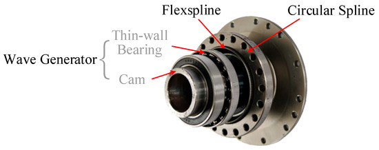
Figure 1.
Scheme of a general harmonic drive.
For a general harmonic drive, the WG serves as the input, either the FS or the CS is the output, and the other one is fixed to the ground. When the FS is fixed, the CS outputs in the same direction as the WG, with its angular velocity [5]; when the CS is fixed, the FS rotates in the direction opposite to the WG, with its angular velocity given by , where ωn is the angular velocity of the WG, and nf and nc are the numbers of teeth on the FS and CS, respectively [5]. Referring to the above equations of angular velocity, closely matched tooth numbers nf and nc lead to a high instantaneous transmission ratio. Without loss of generality, the case where the FS is fixed is considered.
2.2. Equivalence of the Harmonic Drive
To address the modeling complexity, some reasonable equivalences are applied to reduce the degrees of freedom (DoFs) of the harmonic drive, guided by the kinematic relation among its five components (cam, rings of bearing, rollers, FS, and CS). Due to the interference fit effect, the inner ring of the bearing and the cam are treated as a single rigid body, called “equivalent cam (EC)”. In addition, the bearing rollers roll without sliding, and there is no relative sliding on the outer ring. Likewise, there is no relative sliding between the outer race of the thin-wall bearing and the FS, so they are regarded as a single entity, called an “equivalent FS (EFS)”.
Based on the equivalence, the EC contacts with the EFS through rollers, while the EFS further interacts with the CS through multi-tooth engagement. The interactions between EC-EFS and EFS-CS are treated as equivalent stiffness damping, thus obtaining the lumped-parameter model of the harmonic drive, as shown in Figure 2.
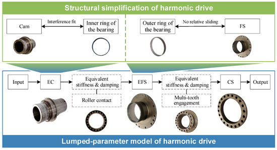
Figure 2.
Framework of the novel harmonic drive model.
3. Contact Mechanics Modeling
Two kinds of contact forces are analyzed in the simplified harmonic drive. One is the meshing force between the EFS and the CS, and the other originates from rollers located between the EFS and the EC. The EFS is simultaneously subjected to the two forces, as shown in Figure 3. An absolute coordinate system OXY and a rotating coordinate system OX’Y’ are marked. The OY-axis is fixed to the ground, and the OY’-axis coincides with the major axis of the EC. With the rotation of the major axis, the OX’Y’ changes an angle of ωnt relative to the OXY. Although the EFS is fixed to the ground, the meshing position changes periodically with the rotation of the EC, so the major axis of the EFS is also rotating. The meshing force is distributed across several gear teeth, where its radial and tangential components are denoted as qr and qt, respectively. The contact force Fri is the radial force applied on the EFS through the i-th roller.
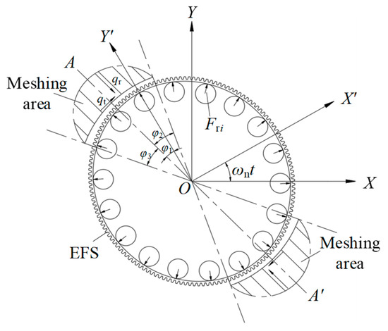
Figure 3.
Forces imposed on EFS.
3.1. Model of Meshing Force
3.1.1. Derivation of Continuously Distributed Meshing Force
As illustrated in Figure 4a, where the red dots represent the meshing points, the meshing force is distributed across the meshing area and nearly symmetrically separated by the AA’-axis. φ1 denotes the angle by which the AA’-axis lags behind the OY’-axis in the clockwise direction; φ2 and φ3 correspond to the half angle of the meshing area. It is assumed that an arbitrarily distributed meshing force is located at a position that lags φ in the clockwise direction from the OY’-axis. According to the previous research, φ2 approximates to φ3, and the distributed meshing forces qt and qr are [26]
where ; and denote the tooth width and the pitch diameter of the CS, respectively; α is the tooth profile angle; and T is the load of the harmonic drive.
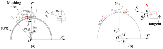
Figure 4.
Contact force between EFS and CS: (a) continuous form; (b) discretized form.
Based on Equation (1), the meshing force along the normal direction of the tooth face can be obtained by
Note that the meshing force described by Equations (1) and (2) is continuously distributed across the meshing area. However, the load is only applied on one side of the gear tooth, and the mesh force is not distributed continuously, as shown in Figure 4b. The mesh force of the ith tooth is obtained by an integration of the distributed force along one tooth pitch, expressed as [27]
where ϕi denotes the angle between the ith tooth and the OY’-axis; ∆ϕ is the angle covered by the i-th tooth.
3.1.2. Composition of Discretely Distributed Meshing Forces
To compose all mesh forces, forces around one end of the major axis are equivalent to a virtual force applied at the end point of the axis. An additional torque M1 is then generated. Assume that the virtual force can be decomposed into two components Fx1 and Fy1, along the OX’ and OY’-axis, respectively. Therefore, Fx1, Fy1, and M1 can be determined by
where xi1 and yi1 are the coordinates of the ith tooth in OX’Y’; βi is the angle between the meshing force of the ith tooth and OX’-axis; and m is the number of the engaged teeth. According to the geometric relation, βi can be calculated by the following equations:
where a and b are defined as the half-length of the major and minor axes, respectively; θ is the angular position of the gear tooth in OX’Y’; ρ is the distance between the gear tooth and the circle center; x denotes the coordinate of the gear tooth along OX’-axis; and h is the slope of tangent from the position of the gear tooth on the EFS.
3.1.3. Equivalent Meshing Stiffness Between EFS and CS
According to the above analysis, the meshing force between the EFS and the CS is modeled as a spring–damper system, as illustrated in Figure 5. By combining Equations (3)–(5), the following equations are obtained:
where δfc is the spring displacement caused by the equivalent force loaded on the spring. Then, the parameters of the spring-damper system, including statistical gear mesh stiffness kfc, the angle αfc of the equivalent virtual force, and the effective radius rfc can be solved.
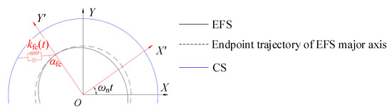
Figure 5.
An equivalent model of the mesh effect.
In Equation (6), kfc is constant as it is solved under a quasi-static condition. Under the circumstances where the harmonic drive operates or the load changes, kfc becomes variable [14]. To accurately describe the dynamic features of a harmonic drive, an in-depth discussion of meshing stiffness should be carried out.
Harmonic drives are frequently utilized in industrial robot joints, where a cyclic inertial load is imposed. The load is time-varying, i.e.,
Parameters related to the meshing area (e.g., φ1, φ2, φ3) and the shape of the EFS also change. Furthermore, how these parameters change over time is hard to express. Seeking the precise expression of the time-varying meshing stiffness kfc(t) is challenging. However, due to the periodicity of T(t), the meshing stiffness should be periodic. Then, kfc(t) can be expanded to the Fourier series with the fundamental frequency of the output frequency fc, expressed as
where km and ψm denote the Fourier coefficient and phase of the mth harmonic, respectively; the static meshing stiffness kfc obtained by Equation (6) is the mean value of kfc(t).
3.2. Model of Roller Contact Forces
The EC contacts with the EFS through rollers, as shown in Figure 6a. When operating, the EFS is deformed to the position of the solid line in Figure 6a, and its major axis rotates with the EC. It is assumed that the angular position of the roller remains the same in the absolute coordinate system, no matter whether the EFS is deformed.
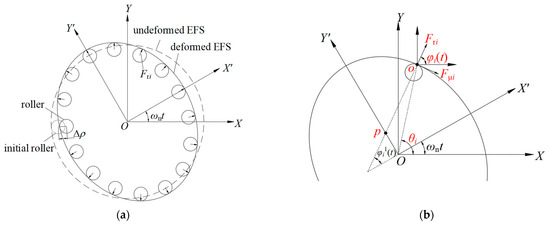
Figure 6.
Contact of EFS and rollers: (a) roller forces; (b) geometric relation of roller forces.
3.2.1. Contact Force Derivation of One Roller
Based on the assumption of rolling without sliding, the radial support force Fri(t) and the tangential friction force Fμi(t) at roller i are written as
where ∆ρi(t) denotes the deformation of the EFS at roller i; kf is the elastic stiffness of the EFS, which is determined by the material and shape; and μ denotes the friction coefficient between the roller and the EFS. The operation max [∆ρi(t),0] means that roller i, which disengages away from the raceway, bears no load when the corresponding part of the EFS is under-stretched and deformed [i.e., ∆ρi(t) < 0].
According to the polar coordinate equation of the ellipse, ∆ρi(t) can be calculated by
where R is the radius of the undeformed EFS and θi denotes the angular position of the center of the ith roller in OXY, as shown in Figure 6b.
The radial and tangential friction forces Fri(t) and Fμi(t) of a single roller are symbolized in Figure 6b. The roller contacts the EFS at point “o”, and the radial force meets the OY-axis at point “p”. The point “p” is the center of curvature of the arc length located by the roller; φi(t) is Fri(t). When the EFS is undeformed, the point “p” coincides with the origin of the coordinate system, and φi(t) equals θi. In Figure 6b, φi(t) does not equal θi because of the deformed EFS.
3.2.2. Contact Force Composition of Rollers
All contact forces of the rollers are equivalent to a composite force and torque at the origin of OXY. The forces Fx(t) and Fy(t) projected to the coordinate axes and the torque M(t) satisfy
where m is the number of rollers; xi(t) and yi(t) are the absolute coordinates of the i-th roller, expressed as
The parameter φi(t) in Equation (11) can be derived by the geometric analysis, which is
where xi1(t) and yi1(t) are the coordinates of the ith roller in the OX’Y’; hi1(t) is the slope of the radial support force of the ith roller in the OX’Y’; and Γ(yi1) denotes a piecewise function, defined as .
3.2.3. Equivalent Stiffness of Roller Contact Between EFS and EC
The composite contact forces of rollers between the EFS and the EC can be regarded as spring–damper systems in 3 DoFs, as shown in Figure 7. Referring to Equation (11), the stiffnesses kwfx(t), kwfy(t), and kwfτ(t) of the three equivalent springs are
where rwf is the effective radius of the torsional spring; is the average deformation of the circumferential points of the EFS, obtained via geometric analysis:
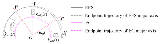
Figure 7.
An equivalent model of contact between EFS and EC.
The three stiffnesses are related to the position of the EC, as shown in Figure 7. Due to the centrosymmetric structure of the cam, the EC meets the initial position after half a rotation, and the stiffness can be described by a function with a period of 1/(2fn). Therefore, kwfx(t), kwfy(t), and kwfτ(t) are expressed as Fourier series, i.e.,
where fn is the input frequency; kln and ψl (l = x, y, or τ) denote the Fourier coefficient and the phase of the nth harmonic, respectively; and kl0 is the mean value of the equivalent stiffness.
4. Dynamic Model of the Harmonic Drive
Building on the contact force models between the components established in Section 3, their equivalent stiffnesses kfc(t), kwfx(t), kwfy(t), and kwfτ(t) are marked in green in Figure 8. Then, the entire harmonic drive is considered as a lumped-parameter model with 9 DoFs, corresponding to the three components (EC, EFS, and CS), as shown in Figure 8. Each component possesses 3 DoFs: two translational (X- and Y-axes) and one rotational (about Z-axis). The three components are supported by housing through bearings and connected to the load or motor by elastic connectors. Each of them can be considered as two perpendicular spring–damper systems and one torsional spring–damper system, whose parameters are symbolled in black in Figure 8.

Figure 8.
Lumped-parameter model of harmonic drive (the dashed lines indicate the trajectories of the rotating major axes).
In the rotating meshing area, gear meshing is modeled as a spring–damper system fixed in the rotating coordinate system OX’Y’, as the red lines illustrated in Figure 8. The rest of the spring–damper systems are fixed in the absolute coordinate system. Installation errors efc1 and efc2 indicate the deviation originated from the manufacturing and assembly process, as symbolized in red in Figure 8. Note that the installation error constitutes one of the excitation sources in the following analysis.
4.1. Excitation Analysis on Installation Errors
It is assumed that the eccentricity occurs in the assembly process and causes installation errors. It differs in the meshing states of the ends of the major axis. For instance, when the eccentricity happens along the direction of the major axis, the EFS will mesh more tightly on one side and more loosely on the other. As the EC rotates, the meshing state transitions back and forth between the two sides. During this process, the contact force between the EFS and CS changes periodically, which can be attributed to the variation in the installation error. Next, the relationship between the eccentricity and the installation error is analyzed. Considering that the eccentricity might happen on the EFS or the CS, it should be discussed in two cases.
- (1)
- Case 1: installation error induced by eccentric EFS
The EFS deviates a length e from the circle center of the EC, as shown in Figure 9a. In the rotating meshing area, an additional displacement eY’(t) is caused by the eccentricity, which is
where the eccentricity is projected to the OY’-axis of the rotating coordinate system.
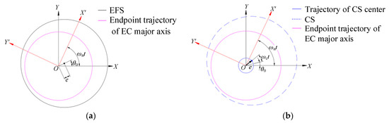
Figure 9.
Equivalent eccentricity of EFS and CS: (a) eccentric EFS; (b) eccentric CS.
Note that the displacement eY’ does not equal the installation error along the direction of tooth engagement. Let their implicit relation be described by a real function f(·) to hold the expression of the installation error at one end of the major axis
Owing to the centrosymmetry of the meshing areas, ef2(t) is opposite to ef1(t) as presented in Figure 8, and there should be a phase lag of π/ωn for ef1(t) to ef2(t):
Referring to Equation (17), and ef1(t) remains periodic, since
Likewise, ef1(t) obeys Therefore, the relation in Equation (18) can be expressed by a periodic function with a minimum period of 2π/ωn, and then be expanded as
where Efn and ϕn denote the Fourier coefficient and the phase of the nth harmonic, respectively; Ef0 is the mean value of the installation error.
- (2)
- Case 2: installation error induced by eccentric CS
It is assumed that the center of the CS is offset by an angle θ0 and a distance e, as illustrated in Figure 9b. Considering the relative angular velocity between the CS and the rotating coordinate system, the additional displacement eY’(t) along the OY’-axis can be described by
Similarly to Case 1, the displacement errors ec1(t) and ec2(t) along the meshing direction are periodic functions with a period of 2π/(ωn − ωc). Therefore, they can be expanded into a Fourier series:
If the EFS and CS become eccentric at the same time, the installation errors efc1(t) and efc2(t) along the meshing direction (shown in Figure 8) are obtained by superimposing Equations (21), (22), (24), and (25),
4.2. Dynamics Differential Equation
According to Newton’s second law, the differential equations of motion of a harmonic drive are derived in the absolute coordinate system. The motion equation of the EC is
The motion equation of the EFS is
The motion equation of the CS is
where xp, yp, and θp (p = w, f, c) represent the translational and rotational coordinates of the equivalent cam, equivalent flexspline, and circular spline in the absolute coordinate system, respectively.
The relative displacement between the EFS and the CS is projected along the direction of the equivalent meshing stiffness, expressed by
Then,
When substituting Equation (30) into Equations (27)–(29), the torsional vibration does not create force in the translational DoF. In other words, torsional and translational vibrations are decoupled. It can be attributed to the structure of the harmonic drive: two centrosymmetric meshing areas are around the rotation center (shown in Figure 9b), and the meshing force induced by translation is centrosymmetric, rendering the equivalent torque to equal 0 in theory
4.3. Characteristics of Vibration Response
In Equations (27)–(29), the motion equations described in translational DoFs possess identical form but different coefficients. Therefore, the responses in the direction of horizontal and vertical present the same frequency characteristics but different amplitudes. Without loss of generality, the motion in the direction of the OY-axis is analyzed. Its motion equation of the EFS satisfies
Substitute Equation (30) into Equation (31), ignore the damping, and decompose Equation (31) into
where excitation sources of the system are moved to the right side of the equation. Specifically, the first term, denoted by f1(t), represents the cyclic load and eccentricity excitation, while the others are derived from the response of the second-order system. To obtain the approximate solution of Equation (31), it is necessary to separately analyze the response under the four excitations in Equation (32).
4.3.1. Cyclic Load and Eccentricity Excitation
When an industrial robot grabs or releases an object, a cyclic inertial load will be applied to the harmonic drive inside the arm of the robot. On one hand, according to Section 3.1, this time-varying load T(t) described by Equation (7) drives kfc(t) to be periodic as Equation (8), acting as an excitation of the harmonic drive; on the other hand, the displacement of kfc(t) represents excitation from the eccentricity. Then, the cyclic load and eccentricity excitation are rewritten as
with which the Fourier transform of f1(t) yields
where denotes convolution. According to Equation (8), Kfc(f) is
where δ(·) is the Dirichlet function. Kfc(f) contains a direct component and multiple harmonics with the output frequency fc as the fundamental frequency, as shown in Figure 10a.
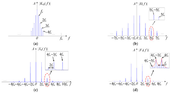
Figure 10.
Frequency characteristics of eccentricity excitation under time-varying load: (a) Kfc(f); (b) E(f); (c) Xe(f); (d) F1(f).
Assume e(t) = efc1(t) − efc2(t), and according to Equation (26), e(t) is then rewritten as
Performing a Fourier transform on Equation (36) yields
Therefore, the Fourier transform of Xe(f) reads
According to Equation (37), E(f) contains two groups of frequency components, as shown in Figure 10b. One is the sum of the odd-order harmonics with the input frequency, fn, as the fundamental frequency; the other is the sum of the odd-order harmonics, with fn − fc as the fundamental frequency, representing the difference between the input and output frequencies. As the order rises, the amplitude of the components decreases rapidly, but the interval between the two groups of frequency components becomes larger. It makes them distinguishable. The convolution in Equation (38) has the spectral line of a single harmonic to be reconstructed around the components of E(f). As a result, the frequency components originally distributed at the odd multiples of fn shift to the even ones, with components at nfn, nfn − (n − 1)fc, and nfn − (n + 1)fc in Xe(f) (n is even), as shown in Figure 10c.
The cyclic load and eccentricity excitation F1(f) is equal to the convolution between the Kfc(f) and Xe(f). The carrier frequency is the component of Xe(f) located at nfn, nfn − (n − 1)fc, and nfn − (n + 1)fc (n is even), while the modulation frequency is a multiple of the output frequency. The characteristic of F1(f) is obtained and presented in Figure 10d. The sidebands around the even-order input frequency comprise a double-peak shape, which is more obvious in the higher-order frequency band. It is caused by the modulation of Kfc(f) around Xe(f), and Xe(f) has two groups of components [nfn and nfn − (n − 1)fc] with a large interval in the high-order frequency band.
4.3.2. Feedback Excitation
In general, the unknown high-frequency components induced by nonlinear behavior exhibit no definitive physical significance. Given that this investigation focuses on revealing the dynamic behavior and frequency distribution of the harmonic drive within the frequency range relevant to practical engineering applications, those high-frequency components caused by nonlinear vibration response have been disregarded [28]. The nonlinear vibration feedback from the other DoFs is treated as 0, and only the known vibration response of the DoF yf is considered. Thus, the 4th excitation term is not concerned. According to Equation (32), the nonlinear excitation induced by the feedback from yf is
When only the linear excitation force f1(t) is applied to the system, the response shows the same features as F1(t) according to the frequency response characteristic of the linear vibration system. Therefore, the Fourier transforms of nonlinear excitations can be expressed as
Based on Equation (16), the Fourier series of kwfy(t) can be expressed as
Hence, the equivalent stiffness kwfy(t) between the EFS and the EC contains a direct component and multiple even-order harmonics with the fundamental frequency of the input frequency fn, as shown in Figure 11a.
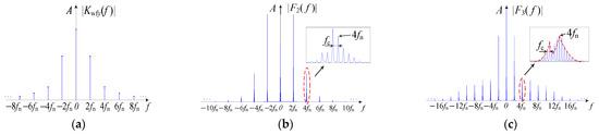
Figure 11.
Frequency characteristic of nonlinear excitation under time-varying load: (a) Kwfy(f); (b) F2(f); (c) F3(f).
The frequency characteristics of F2(f) and F3(f) are manifested in Figure 11b,c, respectively. Both of their sidebands are spaced by fc around nfn, nfn − (n − 1)fc, and nfn − (n + 1)fc (n is even). Due to the feedback vibration, the components of F2(f) and F3(f) are distributed in a wider range than F1(f) but with a smaller amplitude.
Overall, the translational vibration response of the EFS includes the modulation at multiples of the output frequency around nfn, nfn − (n − 1)fc, and nfn − (n + 1)fc (n is even). In Figure 11c, there are only two groups of sidebands presented by the double-peak shape. This is because the components nfn − (n − 1)fc and nfn − (n + 1)fc are very close to each other, and their interval does not change with the order.
5. Simulation
5.1. Parameter Settings of the Proposed Dynamic Model
The FS and CS have 200 and 202 teeth, respectively. It is worth mentioning that revealing the frequency distribution of the vibration response in the frequency domain is more significant instead of their ranges or amplitude. Therefore, some constant simulation parameters are set manually, and some time-varying parameters are determined by selecting the coefficients and orders of the Fourier series. The specific value is explained as follows.
The pitch circle of the CS is 0.0647 m. After the assembly, the major axis of the FS is measured as 0.062 m, and the minor axis is 0.057 m. The effective radius of the contact force between the EFS and EC, namely rwf, is measured as 0.048 m. The material of the model is assigned as steel, and the inertia parameters are listed in Table 1. For the Fourier series of installation errors, the order is set as 10, and the Fourier coefficients are listed in Table 2. The parameters of the spring–damper system connected to housing are presented in Table 3 and Table 4.

Table 1.
Inertia parameters of the simulated harmonic drive.
Table 2.
Fourier coefficient of installation error.
Table 3.
Stiffness of the spring connected to the housing.
Table 4.
Damping of the damper connected to the housing.
Based on Equation (14), the equivalent stiffnesses of EFS-EC are acquired with an input speed of 3000 rpm, as illustrated in Figure 12. Within 700 Hz, there are direct components and harmonics of seven orders whose fundamental frequency is twice the input frequency. Some harmonics are not shown in Figure 12a,c due to the small amplitude. It is consistent between the simulation calculation and theoretical analysis that the equivalent stiffness between EFS-EC mainly contains the even order of the input frequency.
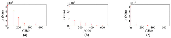
Figure 12.
Equivalent stiffnesses of EFS-EC with input speed of 3000 rpm: (a) kwfx; (b) kwfy; (c) kwft.
Under the condition of a time-varying load, the output load is described by 80 cos(2πfct) N·m. Assume that the static displacement δfc along the equivalent stiffness of EFS-CS is 0.001 m. Based on Equation (6), kfc, αfc, and rfc are calculated as 241,890 N/m, 0.025 rad, and 0.0603 m. The meshing damping is set as 0.1. Hence, the meshing stiffness is expressed by
5.2. Result Analysis
The vibration response of the simulated harmonic drive under the time-varying load is solved via the Runge–Kutta method. As shown in Figure 13, it is composed of two groups of components:
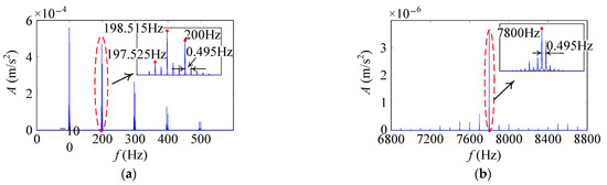
Figure 13.
Translational vibration response of the EFS (time-varying load, input speed 3000 rpm): (a) low frequency components; (b) high frequency components.
- (i)
- the carrier frequencies of nfn, nfn − (n − 1)fc and nfn − (n + 1)fc;
- (ii)
- the modulation frequencies of integer multiple orders of fc.
In Figure 13a, the amplitude of the sidebands in the low-frequency domain decreases with increasing frequency. In the high-frequency domain shown in Figure 13b, the sidebands are amplified immediately because of the resonant peaks in the frequency response function.
To manifest the influence of the vibration feedback, the frequency spectrum with a logarithmic amplitude scale is presented in Figure 14. The result indicates that the spectrum is almost occupied by the sidebands located around the even orders of the input frequency. The sidebands have a more complex distribution, and their amplitude decreases with the increase in order. That is because the components originated from the cyclic load and eccentricity excitation expand to a higher order under the effect of feedback.
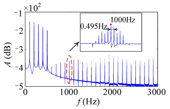
Figure 14.
Log-spectrum of translational vibration response.
In general, the simulation results are consistent with the conclusion of the theoretical analysis.
6. Experiment
To verify the effectiveness of the model, experiments under four different conditions are conducted on the test rig shown in Figure 15, with the experimental conditions listed in Table 5. The test rig contains a harmonic drive, a servo motor for driving, and several mass blocks for loading. The experimental setup employs a DHSG-17-100-U-H19 harmonic drive with a reduction ratio of 100:1, consisting of a circular spline with 202 teeth and a flexspline with 200 teeth. The drive system is actuated by a Delta ECMA-CA0807RS AC servo motor controlled through a Delta ASD-A2-0721-M driver, with control implemented using ASDA-Soft-V5.5.0.0 software. The motor is set to a constant speed. Mass blocks are connected to the CS by a swing arm so that a time-varying inertial load can act on the harmonic drive during operation. An acceleration sensor is located at the top of the harmonic drive housing and collects the vertical vibration with a sampling frequency of 51,200 Hz.
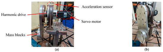
Figure 15.
Harmonic drive test rig: (a) front view; (b) side view.
Table 5.
Four sets of experimental conditions.
6.1. Vibration Signal Analysis
- (1)
- Vibration response in Exp. 1
The vibration signal acquired in Exp. 1 is presented in Figure 16a. Its frequency spectrum in Figure 16b deviates from empirical expectation, as there are almost no components located around the meshing frequency of the harmonic drive (meshing frequency is 10,000 Hz). This phenomenon validates the meshing stiffness model described in Section 3.1. Distinct from traditional gear systems, where meshing-frequency components dominate vibration spectra, the harmonic drive exhibits negligible responses at its meshing frequency. This is because meshing stiffness variation influenced by the number of meshing tooth pairs is not the main internal excitation of the harmonic drive.
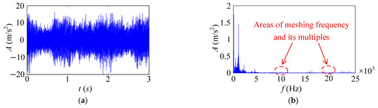
Figure 16.
Vibration signal of Exp. 1: (a) time domain; (b) frequency domain.
The frequency spectrum of the vibration signal is enlarged to manifest the details of the sideband distribution, as shown in Figure 17. The figures reveal that the vibration response is occupied by components located at the even orders of input the frequency, such as 100 Hz, 200 Hz, and 300 Hz. In addition, there are clusters of sidebands gathered around each even order of the input frequency. The carrier frequencies are nfn (200.05 Hz, 400.05 Hz, and 500.05 Hz), nfn − (n − 1)fc (198.52 Hz, 396.59 Hz, and 495.60 Hz), and nfn − (n − 1)fc (197.53 Hz, 395.60 Hz, and 494.61 Hz). The modulation frequencies are fc (0.495 Hz) and its harmonics. However, there are some components distributed around the odd order of the input frequency, which is different from the simulation one. The reason is that manufacturing errors exist in the actual scene, and the two meshing regions are not strictly centrosymmetric to offset the odd-order frequencies. In Equation (16), if the angle between ef1(t) and ef2(t) is not π rad, the relative installation error e(t) in Equation (36) will contain other components besides the odd order of the input frequency. Therefore, these additional components will be modulated by a single harmonic in the cyclic load and eccentricity excitation, and moved to the odd-order input frequency again.
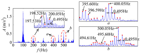
Figure 17.
Enlarged view of the signal in Exp. 1.
- (2)
- Vibration response in Exp. 2
In addition, Exp. 2 with an input speed of 4000 rpm was conducted, and the vibration signal is shown in Figure 18. Similarly, frequency components with sizable amplitudes appear at the carrier frequency of nfn (266.67 Hz, 533.33 Hz and 666.67 Hz), nfn − (n − 1)fc (264.69 Hz, 528.75 Hz and 660.78 Hz) and nfn − (n − 1)fc (263.37 Hz, 527.43 Hz and 659.46 Hz), as well as the modulation frequency of 0.66 Hz. Due to the increase in input speed, both the input and output rotational frequencies varied compared to the signals in Exp. 1, but the frequency distribution pattern remained unchanged.
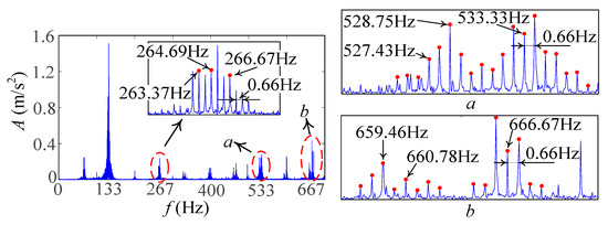
Figure 18.
Enlarged view of the signal in Exp. 2.
- (3)
- Vibration responses in Exp. 3 and Exp. 4
To further validate the reliability of the model, Exp. 3 and Exp. 4 have been conducted on harmonic drives of different transmission ratios. The acquired vibration signals are shown in Figure 19 and Figure 20, respectively. Since the input speed remains constant, the carrier frequencies of both are the same as those in Exp. 1, while the modulation frequencies are 0.98 Hz, 0.41 Hz, with their multiples.
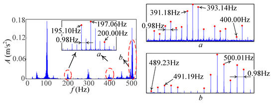
Figure 19.
Enlarged view of signal in Exp 3.
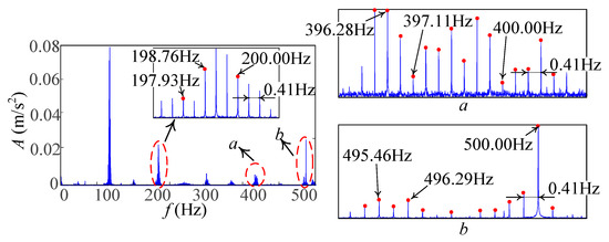
Figure 20.
Enlarged view of the signal in Exp. 4.
In general, an intriguing discovery is that the vibration response caused by the variation in meshing stiffness is slight, which differs in its frequency distribution characteristics from that of common gear systems. In addition, regardless of variations in rotational speed or transmission ratio, the key frequency components of the harmonic drive vibration response include nfn, nfn − (n − 1)fc and nfn − (n + 1)fc, as well as sidebands modulated by fc and its harmonics. Therefore, the experimental signals under different conditions contain key vibration features consistent with those in the simulation and theoretical analyses.
6.2. Discussion
In the vibration signals of the same harmonic drive in Exp. 1 and Exp. 2, the amplitude of the sidebands around 1000 Hz abruptly increases, as shown in Figure 21. This phenomenon is not influenced by operation speed and can be attributed to the feedback amplified around the resonance peak near 1000 Hz.
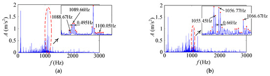
Figure 21.
Frequency spectra of experimental signals: (a) Exp. 1: under the input speed of 3000 rpm; (b) Exp. 2: under the input speed of 4000 rpm.
To verify the correctness of the attribution, the transfer function of the tested harmonic drive has been measured, as shown in Figure 22a, and Figure 22b shows the corresponding coherence coefficients. A natural frequency at 1008 Hz is observed, confirming the accuracy of the analysis. Since the excitation point was arbitrarily chosen and cannot represent the actual operating conditions, Figure 22 only reveals the natural frequencies and does not reveal that higher natural frequency amplitudes correspond to larger vibration response amplitudes.
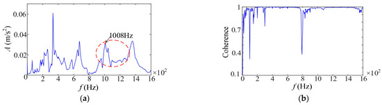
Figure 22.
Test rig frequency response function and coherence coefficients: (a) frequency response function; (b) coherence coefficients.
7. Conclusions
In this study, a dynamic modeling method is proposed to explore the vibration features of the actual harmonic drive response. The proposed method includes three parts: structural simplification, contact mechanics analysis, and system dynamics modeling. The contact mechanics analysis constructs two force models to reflect important features of the interaction among the components. A dynamic model of the whole harmonic drive system is established based on the lumped-parameter method, by considering the installation errors caused by assembly eccentricity as an important excitation. Under time-varying load conditions, the vibration signal of the harmonic drive is simulated, whose significant vibration features are outlined as follows.
- (1)
- There is little meshing component in the vibration response of the harmonic drive. The reason is that many teeth participate in the meshing process, and the meshing stiffness changes little as the tooth alternates.
- (2)
- Under time-varying load, the vibration response contains the carrier frequency located at nfn, nfn − (n − 1)fc, and nfn − (n + 1)fc, as well as the modulation frequency of multiple output frequencies.
These findings provide promising insights into the fault diagnosis of harmonic drives. It is worth further studying the dynamic behavior of the harmonic drive by considering the flexible transfer path of the system and the influence of under-faulty states.
Although the simplified model retains the main interaction characteristics of the original system, the approximate equivalent calculations lead to certain numerical deviations between the simulation and experimental results. Accurate quantification of the equivalent stiffness among components to achieve better consistency between simulation and experimental results requires further investigation. Moreover, the effect of meshing point distance variation on meshing parameters under assembly errors has not been considered, which may influence the vibration response characteristics under normal conditions. This limitation will be addressed in future studies. In addition, the influence of eccentricity on the meshing regions at both ends of the major axis of flexspline has not been fully analyzed, which may explain the response components at odd multiples of the input rotational frequency. This aspect will be further investigated in future studies.
Author Contributions
Conceptualization, G.H.; methodology, G.H. and L.X.; software, B.Z. and Z.Z.; validation, B.Z.; resources, G.H.; writing—original draft preparation, Z.Z.; writing—review and editing, G.H., B.Z. and Y.Z.; visualization, B.Z. and Y.Z.; supervision, H.L.; project administration, H.L. and L.X.; funding acquisition, G.H. All authors have read and agreed to the published version of the manuscript.
Funding
This research was partly supported by the National Key Research and Development Program of China, grant number 2024YFB4709200, the National Natural Science Foundation of China, grant number 52575112, and the Natural Science Foundation of Guangdong Province-China, grant number 2025A1515011145.
Data Availability Statement
The raw data supporting the conclusions of this article will be made available by the authors on request.
Conflicts of Interest
The authors declare no conflicts of interest.
Abbreviations
The following abbreviations are used in this manuscript:
| FS | flexspline |
| WG | wave generator |
| CS | circular spline |
| DoF | degrees of freedom |
| EC | equivalent cam |
| EFS | equivalent flexspline |
Nomenclature
The following symbols are used in this article:
| ωn | Angular velocity of the wave generator (WG). |
| nf, nc | Tooth numbers of the flexspline (FS) and circular spline (CS). |
| a, b | Half-lengths of the major and minor axes of the flexspline ellipse. |
| R | Radius of the undeformed equivalent flexspline (EFS). |
| OXY | Absolute coordinate system fixed to the ground. |
| OX’Y’ | Rotating coordinate system whose Y’-axis coincides with the major axis of the equivalent cam (EC). |
| θi, ϕi | Angular positions of the i-th roller or tooth in the coordinate system. |
| hi | Slope of the tangent at the i-th contact point on the EFS. |
| xp, yp, θp | Translational and rotational displacements of component p (p = w, f, c: EC, EFS, CS). |
| rwf, rfc | Effective radii of roller contact and meshing contact. |
| α | Pressure angle of the tooth profile. |
| qt, qr, qz | Tangential, radial, and normal components of distributed meshing force. |
| qt,max | Maximum tangential component of distributed meshing force. |
| fi | Meshing force acting on the i-th tooth. |
| Fx1, Fy1 | Equivalent force components along the X’- and Y’-axes. |
| M1 | Equivalent torque generated by discretely distributed meshing forces. |
| Fri(t) | Radial contact force on the i-th roller between the EFS and EC. |
| Fμi(t) | Tangential friction force on the i-th roller. |
| Fx(t), Fy(t), M(t) | Resultant forces and torque obtained by superimposing all roller forces. |
| ∆ρi(t) | Radial deformation of the EFS at the i-th roller. |
| Average deformation of the circumferential points of the EFS. | |
| μ | Friction coefficient between the roller and the EFS. |
| kf | Elastic stiffness of the EFS material. |
| kfc(t) | Time-varying meshing stiffness between EFS and CS. |
| kwfx(t), kwfy(t), kwfτ(t) | Equivalent stiffnesses of the roller contact between EFS and EC in X, Y, and torsional directions. |
| kpl | Support stiffness of component p (p = w, f, c) in direction l (l = x, y, τ). |
| cpl | Damping coefficient of the support damper for component p in direction l. |
| δpl | Displacement along the direction of the equivalent meshing stiffness. |
| km, ψm | Fourier coefficient and phase of the m-th harmonic of meshing stiffness. |
| kln, ψl | Fourier coefficient and phase of the n-th harmonic for stiffness kwfl(t) (l = x, y, τ). |
| mp | Mass of component p (p = w, f, c). |
| Ip | Rotational inertia of component p (p = w, f, c) about the Z-axis. |
| fn | Input frequency of the wave generator (rotation frequency). |
| fc | Output frequency of the circular spline. |
| fs | Sampling frequency of the experimental data acquisition system. |
| T(t) | Time-varying transmitted torque or cyclic inertial load. |
| e(t) | Installation error or eccentric displacement along the meshing direction. |
| efc1(t), efc2(t) | Periodic installation errors on both ends of the major axis. |
| efn, ecn | Fourier coefficients of installation error harmonics. |
| ϕn | Phase angles of the n-th harmonic in Fourier series expansions. |
| Kfc(f) | Frequency-domain expression of time-varying meshing stiffness. |
| Kfc(f), E(f) | Fourier transforms of excitation displacement and installation error. |
| F1(f), F2(f), F3(f) | Frequency spectra of cyclic load, nonlinear feedback, and overall excitation. |
| rwf | Effective radius of roller contact. |
| bR | Tooth width of the circular spline. |
| dg | Pitch diameter of the circular spline. |
References
- Wang, J.; Wan, Z.; Dong, Z.; Li, Z. Research on Performance Test System of Space Harmonic Reducer in High Vacuum and Low Temperature Environment. Machines 2020, 9, 1. [Google Scholar] [CrossRef]
- Li, F.; Li, X.; Guo, Y.; Shang, D. Analysis of Contact Mechanical Characteristics of Flexible Parts in Harmonic Gear Reducer. Shock. Vib. 2021, 2021, 5521320. [Google Scholar] [CrossRef]
- Mongia, C.; Goyal, D.; Sehgal, S. Vibration Response-Based Condition Monitoring and Fault Diagnosis of Rotary Machinery. Mater. Today Proc. 2022, 50, 679–683. [Google Scholar] [CrossRef]
- Jia, H.; Li, J.; Xiang, G.; Wang, J.; Xiao, K.; Han, Y. Modeling and Analysis of Pure Kinematic Error in Harmonic Drive. Mech. Mach. Theory 2021, 155, 104122. [Google Scholar] [CrossRef]
- Understanding and Modeling the Behavior of a Harmonic Drive Gear Transmission. Available online: https://dspace.mit.edu/handle/1721.1/6803 (accessed on 2 January 2025).
- Li, X.; Song, C.; Zhu, C.; Song, H. Load Analysis of Thin-Walled Flexible Bearing in Harmonic Reducer Considering Assembly with Flexspline and Cam. Mech. Mach. Theory 2023, 180, 105154. [Google Scholar] [CrossRef]
- Trang, T.; Pham, T.; Hu, Y.; Li, W.; Lin, S. A Quick Stress Calculation Method for Flexspline in Harmonic Actuators Based on the Finite Element Method. Cogent Eng. 2022, 9, 2138123. [Google Scholar] [CrossRef]
- Hu, Q.; Li, H.; Wang, G.; Li, L. Research on Torsional Stiffness of Flexspline-Flexible Bearing Contact Pair in Harmonic Drive Based on Macro-Micro Scale Modeling. Front. Mater. 2023, 10, 1211019. [Google Scholar] [CrossRef]
- Li, R.; Zhou, G.; Li, D. Structural Design of Flexible Wheel of Harmonic Reducer Based on Efficiency Improvement. Mech. Syst. Signal Process. 2023, 201, 110677. [Google Scholar] [CrossRef]
- Ghorbel, F.H.; Gandhi, P.S.; Alpeter, F. On the Kinematic Error in Harmonic Drive Gears. J. Mech. Des. 2001, 123, 90–97. [Google Scholar] [CrossRef]
- Xiong, Y.; Zhu, Y.; Yan, K. Load Analysis of Flexible Ball Bearing in a Harmonic Reducer. J. Mech. Des. 2020, 142, 022302. [Google Scholar] [CrossRef]
- Yague-Spaude, E.; Gonzalez-Perez, I.; Fuentes-Aznar, A. Stress Analysis of Strain Wave Gear Drives with Four Different Geometries of Wave Generator. Meccanica 2020, 55, 2285–2304. [Google Scholar] [CrossRef]
- Song, C.; Li, X.; Yang, Y.; Sun, J. Parameter Design of Double-Circular-Arc Tooth Profile and Its Influence on Meshing Characteristics of Harmonic Drive. Mech. Mach. Theory 2022, 167, 104567. [Google Scholar] [CrossRef]
- Ma, J.; Li, C.; Luo, Y.; Cui, L. Simulation of Meshing Characteristics of Harmonic Reducer and Experimental Verification. Adv. Mech. Eng. 2018, 10, 1687814018767494. [Google Scholar] [CrossRef]
- Zhang, Y.; Pan, X.; Li, Y.; Wang, G.; Wu, G. Meshing Stiffness Calculation of Disposable Harmonic Drive under Full Load. Machines 2022, 10, 271. [Google Scholar] [CrossRef]
- Tang, T.; Li, J.; Wang, J.; Xiao, K.; Han, Y. Double-Circular-Arc Tooth Profile Design and Parametric Analysis on the Comprehensive Performance of the Harmonic Drive. Proc. Inst. Mech. Eng. Part. J. J. Eng. Tribol. 2022, 236, 480–498. [Google Scholar] [CrossRef]
- Raviola, A.; De Martin, A.; Guida, R.; Jacazio, G.; Mauro, S.; Sorli, M. Harmonic Drive Gear Failures in Industrial Robots Applications: An Overview. PHM Soc. Eur. Conf. 2021, 6, 11. [Google Scholar] [CrossRef]
- Zhao, J.; Yan, S. Coupling Vibration Analysis for Harmonic Drive in Joint and Flexible Arm Undergoing Large Range Motion. In Proceedings of the 2016 International Symposium on Flexible Automation (ISFA), Cleveland, OH, USA, 1–3 August 2016; IEEE: Cleveland, OH, USA; pp. 442–449. [Google Scholar]
- Masoumi, M.; Alimohammadi, H. An Investigation into the Vibration of Harmonic Drive Systems. Front. Mech. Eng. 2013, 8, 409–419. [Google Scholar] [CrossRef]
- Hu, R.; Zhou, G.; Li, J. A Nonlinear Torsional Vibration Model of Harmonic Gear Reducer and the Effect of Various Factors on Torsional Vibration during Start and Stop. J. Vib. Control 2022, 28, 1536–1549. [Google Scholar] [CrossRef]
- Zhao, X.Z.; Guo, Y.Y.; Li, Z.; Ye, B.Y.; Chen, T.J. Injury Characteristic Frequency Analysis of Flexible Thin-Wall Bearing. J. Vib. Eng. 2020, 33, 1313–1323. [Google Scholar]
- Zhang, X.; Tao, T.; Jiang, G.; Mei, X.; Zou, C. A Refined Dynamic Model of Harmonic Drive and Its Dynamic Response Analysis. Shock. Vib. 2020, 2020, 1841724. [Google Scholar] [CrossRef]
- Yang, X.; Qiang, D.; Chen, Z.; Wang, H.; Zhou, Z.; Zhang, X. Dynamic Modeling and Digital Twin of a Harmonic Drive Based Collaborative Robot Joint. In Proceedings of the 2022 International Conference on Robotics and Automation (ICRA), Philadelphia, PA, USA, 23 May 2022; IEEE: Philadelphia, PA, USA; pp. 4862–4868. [Google Scholar]
- Gu, J.; Tong, T.; Huang, D.; Li, M. Study on Torsional Vibration of a Harmonic Driver Based on Time-Varying Stiffness Caused by Manufacturing Error. J. Vibroengineering 2021, 23, 619–631. [Google Scholar] [CrossRef]
- Shi, J.F.; Han, C.; Chen, L.X.; Jin, W.Y. Investigating Wear-Induced Health-Instability Dynamics in Spur Gear Systems with Installation Error. Nonlinear Dyn. 2025, 113, 22701–22722. [Google Scholar] [CrossRef]
- Ivanov, M.N. The Harmonic Drive; National Defense Industry Press: Beijing, China, 1987. [Google Scholar]
- Zhang, X.; Zhang, C.; Wang, P.; Yang, F.; Peng, C. Stiffness Reliability Analysis of Harmonic Drive Considering Contact Pairs Wear. Eng. Comput. 2024, 41, 1327–1352. [Google Scholar] [CrossRef]
- Li, Y.; Ding, K.; He, G.; Lin, H. Vibration Mechanisms of Spur Gear Pair in Healthy and Fault States. Mech. Syst. Signal Process. 2016, 81, 183–201. [Google Scholar] [CrossRef]


Disclaimer/Publisher’s Note: The statements, opinions and data contained in all publications are solely those of the individual author(s) and contributor(s) and not of MDPI and/or the editor(s). MDPI and/or the editor(s) disclaim responsibility for any injury to people or property resulting from any ideas, methods, instructions or products referred to in the content. |
© 2025 by the authors. Licensee MDPI, Basel, Switzerland. This article is an open access article distributed under the terms and conditions of the Creative Commons Attribution (CC BY) license (https://creativecommons.org/licenses/by/4.0/).