Classification Scheme for the Three-Point Dubins Problem

Abstract

This paper proposes an optimal path type classification scheme for the three-point Dubins problem. It allows us to directly extract the shortest path type from a Dubins set, evaluating only the relative initial and final configurations with the via point position using a suitable partition of the Cartesian plane. Two alternative approaches are proposed to address the problem: an analytical approach and a heuristic one. The latter is revealed to be much faster from a computational point of view. The proposed classification logic makes the path planning for the three-point Dubins problem much more effective and suitable for real-time applications. Numerical examples are provided to show the efficiency of the proposed strategy.

1. Introduction

The technological advances of recent years opened up astonishing possibilities for research. From virtual reality to artificial intelligence and self-driving cars, the promise of a future world where such technologies permeate human society is exciting, and it drives the research in these fields with a renewed and powerful thrust. Among the most fascinating topics, the goal of designing mobile devices that are autonomously able to safely handle human mobility is advancing every day to reality.

In this latter scenario, and other similar ones, a central theme is the autonomy of a device for decision-making, ensuring that robots are able to find feasible paths in various environments, avoiding obstacles and minimizing travel time or energy consumption. For this reason, the challenging problem of safe and autonomous navigation surged as a central topic in robotics and autonomous systems. Overall, path planning is a foundational aspect of robotic vehicle that impacts the performance, safety, and effectiveness of robotic systems across a wide range of applications [1]. In recent years, there has been an impressive surge of research from the AI community (see, e.g., the overview papers [2,3] and references therein).

One key aspect of path planning is producing feasible reference paths for robots, namely, paths that are compliant with robots’ kinematics so that the robots are able to track the paths without jumps or errors.

A fundamental kinematic model that has been extensively explored in path planning applications is the ‘Dubins vehicles’ [4]. Basically, it refers to a point moving in the plane at a constant forward speed and bounded curvature, while the Dubins path refers to the shortest path between two poses of a Dubins vehicle [4]. It is well suited to represent the movement of vehicles that do not require hard braking, slowdown, or stopping; common examples are airplanes or marine crafts. For these reasons, since the milestone contribution by Dubins [5], the Dubins vehicle has been constantly studied over the years, as witnessed by the works in [6,7,8,9]. In these works, Dubins paths are obtained through necessary optimality conditions derived by exploiting the theoretical framework based on Pontryagin’s Maximum Principle. However, this approach results in solutions that are computationally demanding and not readily applicable to real-time applications. A significant contribution to overcome this issue is the work in [10], where the computational complexity is reduced by selecting the optimal path type based only on the initial and final poses (namely, position and orientation) in the Cartesian plane. In recent years, the application of machine learning techniques to the Dubins path planning problem has also been explored [11,12]. Other research areas that have emerged over the years are related to the generalizations of the Dubins problem through N points, as the Dubins Traveling Salesman Problem (DTSP) [13,14,15,16].

Several contributions on this subject [17] have shown that when the order of via points is fixed, the solution of the DTSP can be decomposed at each step in sub-problems, known as the three-point Dubins problem (3PDP), namely the path planning problem for a Dubins vehicle with an intermediate via point [18,19,20].

The three-point Dubins problem leads to efficient navigation solutions in different application domains including air, ground, and marine environments. In the field of Unmanned Aerial Vehicles (UAVs), solving the 3PDP is essential for optimizing flight paths when navigating through constrained environments or for executing complex missions. This can be particularly important in surveillance, reconnaissance, and delivery operations [21]. Even drones used in precision agriculture often need to navigate specific via points. In [22], for example, a variation of the Traveling Salesman Problem (TSP) solver, which is an extension of the 3PDP, is proposed to investigate optimal trajectories in order to visit a specific number of plants that require intervention. Aircraft, especially those with limited maneuverability, may encounter the 3PDP during specific flight scenarios [23], such as air-to-air refueling or navigating airspace restrictions. Efficient path planning is crucial for ensuring safe and precise movements in these situations.

In scenarios where search and rescue missions involve aerial or ground vehicles with Dubins motion constraints, solving the 3PDP with fast algorithms can be a key tool for safe and length-optimal reference path generation. Indeed, these applications often require real-time path planning to reach a target location with an intermediate point, optimizing the trajectory for a quick and effective response [24]. Moreover, Dubins vehicles, such as autonomous cars and ground robots, encounter the 3PDP when planning paths that involve navigating obstacles or following specific via points. Solving this problem is vital for ensuring safe and efficient transportation in urban environments or other constrained spaces [25,26]. In automated warehouses, multiple robots may need to navigate through narrow aisles and around obstacles while efficiently reaching intermediate points for picking or restocking purposes. Solving the 3PDP is a relevant basis for optimizing the movement of robotic vehicles in such environments [27].

Also, autonomous underwater vehicles (AUVs) face challenges in path planning, especially when they need to travel from one point to another with an intermediate via point. The solution of the 3PDP and its extension, Multiple Traveling Sales Person (MTSP), can be applied to optimize their trajectories and conserve energy during underwater missions [28].

In summary, the significance of solving the three-point Dubins problem  (shortened to 3PDP hereafter) lies in its potential to enhance the performance, safety, and efficiency of various autonomous systems operating in diverse real-world applications. This has motivated recent studies on developing increasingly faster and more efficient methods to address the 3PDP [17,18,29]. The solution proposed in [17] is based on inversive geometry. Two methods are presented: an “Approximate Method” that, while computationally efficient, provides an approximate optimal heading at the via-point, and an “Iterative Method” that recursively converges to the exact heading by iterative corrections, thus achieving greater accuracy at the cost of increased computational resources. A significant contribution is found in the work of [18], which utilizes the Pontryagin principle and optimality criteria. This research offers a solution encompassing all possible cases. The method requires solving polynomial equations, ensuring an accurate/exact solution by construction. A promising solution was proposed recently [29]; it is based on novel methodologies related to optimal properties of conic sections. The solution can be computed either graphically or analytically by utilizing the matrix description of conic sections. It provides solutions with an adequate level of accuracy as well as a reduced computational effort. Overall, any existing approach to the 3PDP, despite its peculiar methodology, selects the minimum length path through an exhaustive search among all possible path type combinations. This is detrimental to the run time, and it is a significant drawback for these methodologies when dealing with the applications described above. The main goal of this paper is to remove this bottleneck, thus extending the classification rules from [10] to the 3PDP. This would allow for the direct determination of the optimal path type based on the initial and final poses and the intermediate via point only. As a result, the results of this paper can be applied in conjunction with any algorithm to obtain solutions in real-time applications.

2. Problem Formulation

In the following subsections, we introduce the logical framework of the problem, and we briefly summarize some classical results that are the basis of our analysis, together with the notation that we adopt along the paper.

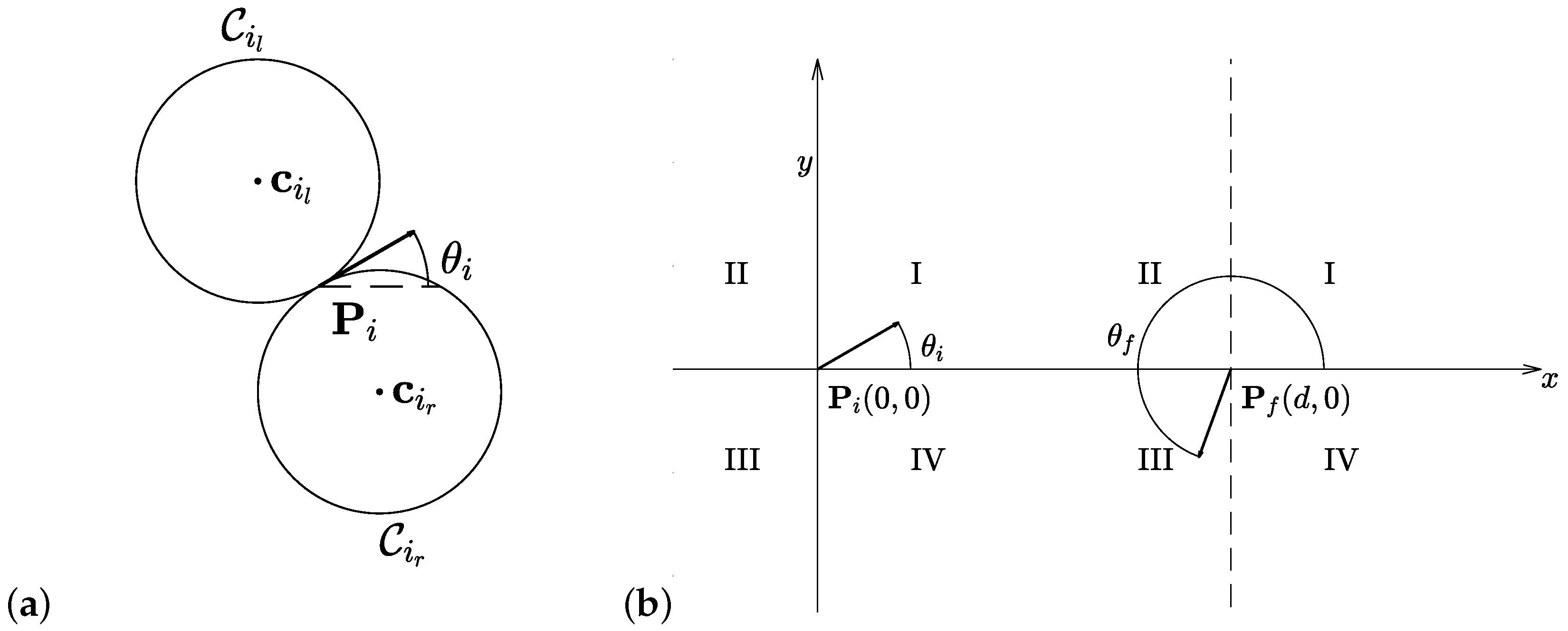
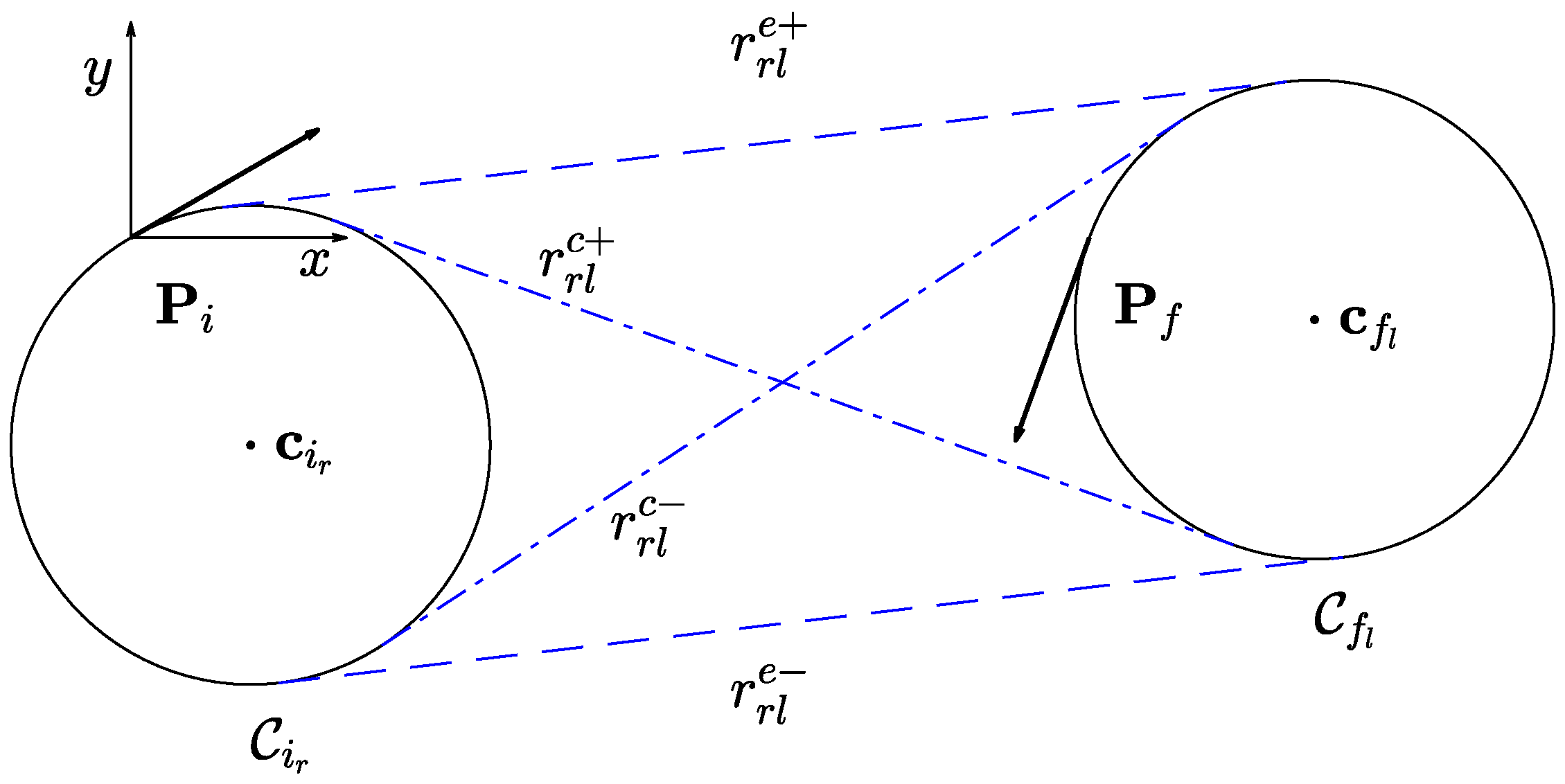
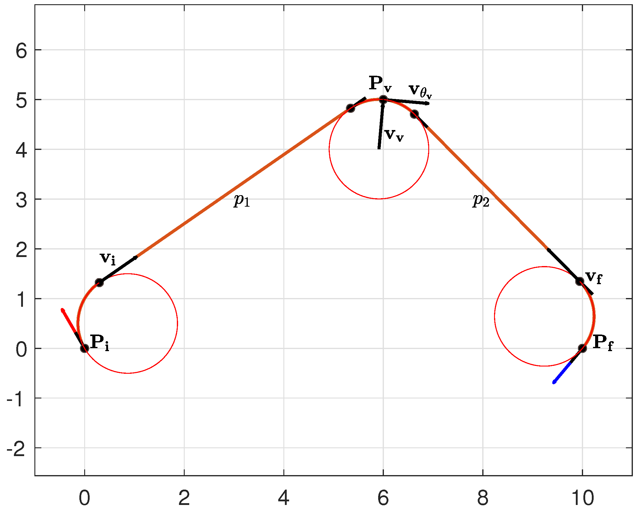
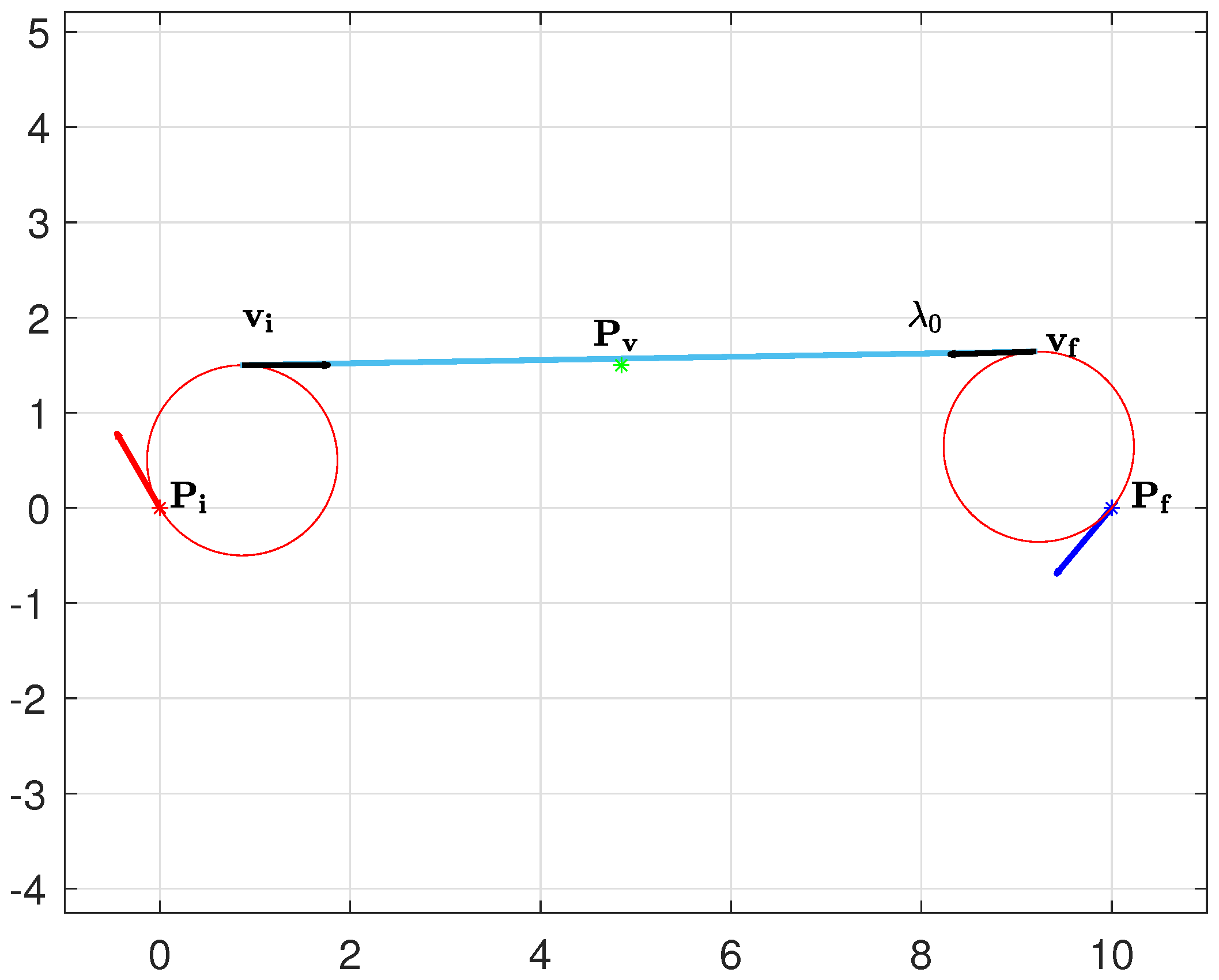
2.1. Notation and Preliminary Results

Consider a vehicle whose motion is described by

$$\left\{\begin{array}{c}\dot{x}=cos\theta ,\hfill \\ \dot{y}=sin\theta ,\hfill \\ \dot{\theta }=u,\hfill \\ \left|\right|u\left|\right|\le \mathrm{\Omega };\hfill \end{array}\right.$$

(1)

where $\mathrm{\Omega }$ is a bound on the maximal curvature. A feasible path is a curve in the plane that is viable for the Dubins vehicle, namely, a curve satisfying (1), whose maximum curvature along the path is bounded by $\mathrm{\Omega }$.

The state vector $\mathbf{q}=(\mathit{P},\theta )$ is the pose or configuration of the vehicle, where $\mathit{P}=(x,y)$ is the position of the vehicle in the Euclidean plane, and $\theta \in [0,2\pi )$ its orientation (see Figure 1a); the control u sets the angular speed, within the range defined by the bound $\mathrm{\Omega }$. Associated to each configuration, we draw two circles of radius ${\mathrm{\Omega }}^{-1}$, each lying on one side of position P (denoted ${\mathcal{C}}_l$ for the left circle and ${\mathcal{C}}_r$ for the right circle, and their centers ${\mathbf{c}}_l$ and ${\mathbf{c}}_r$, respectively), each corresponding to the sharpest turn.

Figure 1. (a) Graphical interpretation of the left and right centers for an initial configuration ${\mathbf{q}}_i=({\mathit{P}}_i,{\theta }_i)$. (b) Initial and final configurations.

Given an initial configuration ${\mathbf{q}}_i=({\mathit{P}}_i,{\theta }_i)$ and a final configuration ${\mathbf{q}}_f=({\mathit{P}}_f,{\theta }_f)$, without loss of generality (as in [10]), it is possible to set ${\mathit{P}}_i=(0,0)$ and ${\mathit{P}}_f=(d,0)$, with d the Euclidean distance between them, as depicted in Figure 1b.

Consider two such circles ${\mathcal{C}}_{a_b}$, with $a\in \mathcal{A}=\{i,f\}$ (namely, “initial” or “final”) and $b\in \mathcal{B}=\{r,l\}$ (i.e., “right” or “left”); it is possible to identify four different common tangent lines, i.e., two cross tangents and two external ones (see, e.g., Figure 2). We denote all possible common tangent lines between an initial and a final circle as $r_{cd}^{ts}$, with $c,d\in \mathcal{B}$, $t\in \{c,e\}$, and $s\in \{+,-\}$ (where c and e stand for “cross” and “external”; + and − for “superior” and “inferior”).

Figure 2. Representation of the common tangents between the circles ${\mathcal{C}}_{i_r}$ and ${\mathcal{C}}_{f_l}$: $r_{rl}^{c+}$, superior cross tangent; $r_{rl}^{c-}$, inferior cross tangent; $r_{rl}^{e+}$, superior external tangent; and $r_{rl}^{e-}$, inferior external tangent.

Consider a line r in the Cartesian plane described by all the points $P=(x,y)$ satisfying $y=m_{r}x+q_r$, (see Figure 3); r divides the Cartesian plane into two half-planes. A point $\mathit{P}=(x_P,y_P)$ is in the upper half-plane if $y_P>m_r{x}_P+q_r$, and it is shortly denoted by $\mathit{P}>r$. The point P is said to be in the lower half-plane if $y_P<m_r{x}_P+q_r$, denoted hereafter by $\mathit{P}<r$.

Figure 3. Notation for the position of a point with respect to a line r and an oriented line (curve) $r_o$.

Finally, each directed line $r_o$ with unit vector ${\mathbf{v}}_{r_o}$ divides the Cartesian plane into two half-planes; the one on its right is shortly denoted as ${\pi }_{r_o}^r$, and the other on its left denoted as ${\pi }_{r_o}^l$. If ${\mathbf{v}}_{r_o}$ points to the right, then ${\pi }_{r_o}^l$ coincides with the upper half-plane.

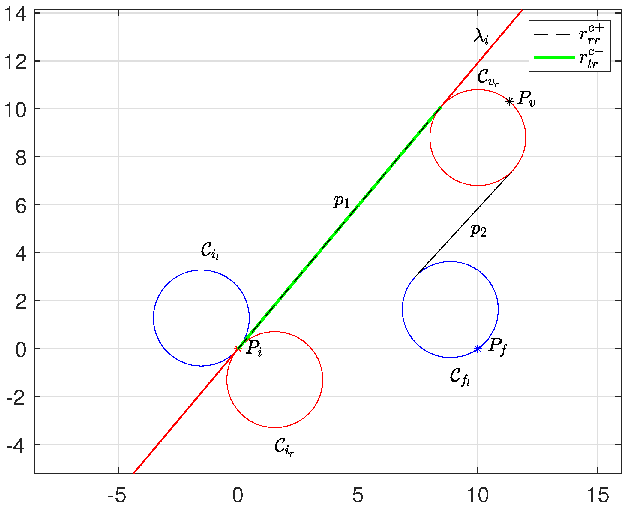
2.2. Preliminary Results

One fundamental topic within this framework is the shortest path problem, which consists in finding the shortest curve among the viable ones connecting an initial configuration ${\mathbf{q}}_i=({\mathit{P}}_i,{\theta }_i)$ to a final configuration ${\mathbf{q}}_f=({\mathit{P}}_f,{\theta }_f)$ for a Dubins car. This problem was firstly introduced and solved by L.E. Dubins [5] by showing that an optimal path is constructed by combining at most three segments, which can be either a straight line (denoted as S) or a circular arc of maximum curvature (denoted as C).

A circular path C can have a right or left turning direction, and hereafter, it is denoted by R or L, respectively. As a consequence, the minimum length path can be found by a direct search among six possible combinations given by the $\{LSL$, $RSR$, $RSL$, $LSR$, $RLR$, $LRL\}$ cases, or part of them. If the distance between the initial and final points is sufficiently large, more than $4{\mathrm{\Omega }}^{-1}$, $CCC$ paths are never optimal, and the analysis can be restricted to the occurrence of $CSC$ paths. Moreover, $CCC$ paths are inconvenient in practice since small variations on the terminal configurations produce large variations of solutions, namely, the recalculation of a reference path may produce a completely different reference path, with possible serious drawbacks on a mission execution.

For these reasons, in this paper, we propose an algorithm that seeks the solution type of the optimal-length Dubins path restricted to a search among the four combinations $\{LSL$, $RSR$, $RSL$, $LSR\}$. When $P_v$ is far more than $4{\mathrm{\Omega }}^{-1}$ both from ${\mathit{P}}_i$ and ${\mathit{P}}_f$, the path type solution is optimal. In general, for most of the practical applications, such path type is the most reasonable choice.

The three-point Dubins problem (3PDP) is as follows. For any assigned triple (${\mathbf{q}}_i$, ${\mathit{P}}_v$, ${\mathbf{q}}_f$), namely, the initial configuration ${\mathbf{q}}_i=({\mathit{P}}_i,{\theta }_i)$, the final configuration ${\mathbf{q}}_f=({\mathit{P}}_f,{\theta }_f)$, and a pre-assigned via point ${\mathit{P}}_v$ far from ${\mathit{P}}_i$ and ${\mathit{P}}_f$ more than $4{\mathrm{\Omega }}^{-1}$, find the shortest curve of (1) connecting ${\mathit{P}}_i$, ${\mathit{P}}_v$, and ${\mathit{P}}_f$, with tangent direction ${\theta }_i$ at ${\mathit{P}}_i$ and ${\theta }_f$ at ${\mathit{P}}_f$, among all the curves in the plane with curvature bounded by $\mathrm{\Omega }$.

According to Bellman’s principle for optimality, the solution of the optimal path for a Dubins vehicle between three consecutive configurations can be obtained by concatenating two optimal Dubins paths:

• The path between the initial configuration ${\mathbf{q}}_i=({\mathit{P}}_i,{\theta }_i)$ and the via point configuration ${\mathbf{q}}_v=({\mathit{P}}_v,{\theta }_v)$ with length denoted as $L_1$, and
• The path between the via point configuration ${\mathbf{q}}_v=({\mathit{P}}_v,{\theta }_v)$ and the final configuration ${\mathbf{q}}_f=({\mathit{P}}_f,{\theta }_f)$ with length denoted as $L_2$.

In this paper, we deduce the classification rules for selecting the type of the optimal path for those points $P_v$ of the plane far from $P_i$ and $P_v$ more than $4{\mathrm{\Omega }}^{-1}$, so that each of the elementary optimal Dubins path must be of type $CSC$; thus, the solution is made of three elementary motions: left or right turn both along a circle of radius ${\mathrm{\Omega }}^{-1}$, straight line motion, and left or right turn both along a circle of radius ${\mathrm{\Omega }}^{-1}$. Hereafter, we denote as t, p, and q the length of its basic elements referring to the initial turn, the straight line segment, and the final turn, and we add the subscript 1 or 2 to refer to the path between ${\mathit{P}}_i$ to ${\mathit{P}}_v$ and from ${\mathit{P}}_v$ to ${\mathit{P}}_f$, respectively; see Figure 4.

Figure 4. A sketch of an $LSL-LSL$ path.

We can, therefore, state that the optimal-length path through three consecutive points satisfying the long distance hypothesis is the concatenation of two Dubins paths of type $CSC$; hence, the solution of the 3PDP must be of type $CSC-CSC$. If such hypothesis is not satisfied, however, one may use a sub-optimal solution of type $CSC-CSC$, thus a priori avoiding $CCC$ curves (which can be optimal, but notwithstanding, inconvenient).

An important result, conjectured in [19], and then proved in [17,30], is related to the optimality conditions for a shortest path of type $CSC-CSC$:

Lemma 1.

Given $({\mathbf{q}}_i,{\mathbf{q}}_f,{\mathit{P}}_v)$; in a shortest path of type CSC-CSC, the line segment between ${\mathit{P}}_v$ and the center of the circle associated with the optimal heading bisects the angle between the line segment $p_1$ and $p_2$.

Denote by ${\mathbf{v}}_i$ and ${\mathbf{v}}_f$ the vectors parallel to the initial and final line segments of path $CSC-CSC$, ($p_1$ and $p_2$ in Figure 4 and Figure 5), and with ${\mathbf{v}}_v$ the vector connecting the center of the circle associated with the optimal heading at the via point ${\mathit{P}}_v$. Define ${\mathbf{v}}_{{\theta }_v}$ as the vector parallel to the optimal heading at the via point, hence orthogonal to ${\mathbf{v}}_v$ by construction, as shown in Figure 5.

Figure 5. The vectors ${\mathbf{v}}_i$, ${\mathbf{v}}_f$, ${\mathbf{v}}_v$, and ${\mathbf{v}}_{{\theta }_v}$ for an $RSR-RSR$ path.

Denoting by $\mathbf{v}$ the vector bisecting the angle between ${\mathbf{v}}_i$ and ${\mathbf{v}}_f$, the optimality condition of Lemma 1 can be equivalently rewritten as follows:

$${\mathbf{v}}^{\top }{\mathbf{v}}_{{\theta }_v}=\mathbf{0}.$$

(2)

Moreover, since two arcs incident on the via point must have the same turning direction, the following holds:

Corollary 1.

The optimal solution of the 3PDP when $P_v$ is far more than $4{\mathrm{\Omega }}^{-1}$ from both $P_i$ and $P_v$ must be of a type in $\mathcal{T}=\{RSR-RSR$, $LSR-RSR$, $RSR-RSL$, $LSR-RSL$, $LSL-LSL$, $RSL-LSL$, $LSL-LSR$, $RSL-LSR\}$, where any circular arc may possibly be of zero length.

As a consequence, the optimal-length path through three consecutive points can be found by direct search among the eight possible combinations in $\mathcal{T}$.

2.3. A Classification Approach for a Fast Solution

In this paper, we propose a classification based on a partition of the Cartesian plane which allows us to drastically reduce the number of potential path types.

Indeed, in order to solve the 3PDP, one should calculate the lengths of all path types in $\mathcal{T}$ and then select the shortest one of the computed paths. This requires one to compute the optimal orientation angle at the via point ${\theta }_v$ (not specified a priori) for each path type, given by the following length optimality criterion:

$${\theta }_v^{\ast }=arg{\min }_{{\theta }_v\in [0,2\pi )}(L_1\left({\theta }_v\right)+L_2\left({\theta }_v\right)).$$

(3)

The problem addressed in this paper can be formulated as follows.

Problem 1.

Given the 3PDP, find a simple logical procedure to select the optimal path type among the combinations given in $\mathcal{T}$ without any explicit length computation.

Inspired by the classification rules derived in [10], in this paper we extend this strategy to the 3PDP: given a 3PDP problem, find a simple logical procedure to select the optimal path type among those in $\mathcal{T}$ without any explicit length computation.

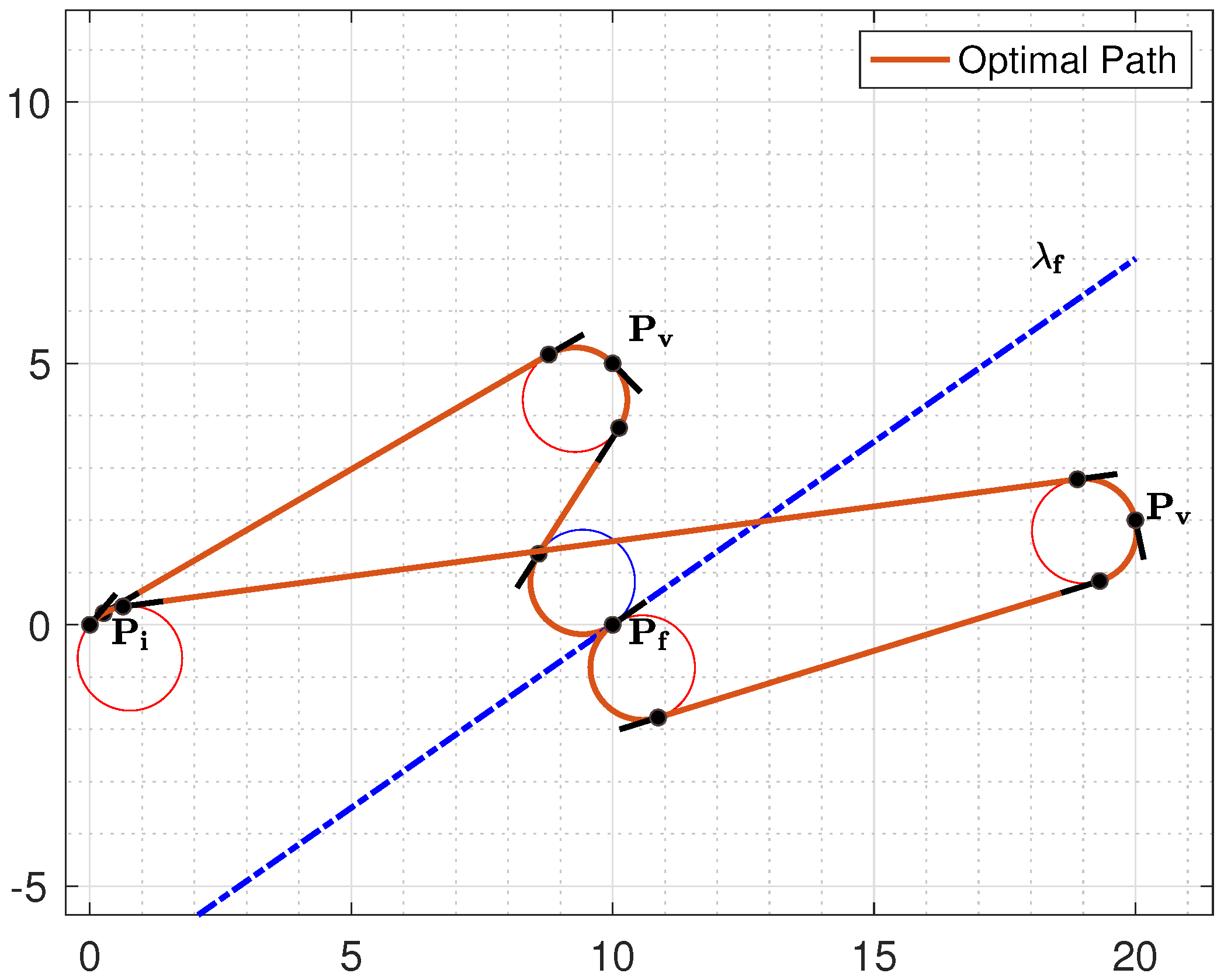
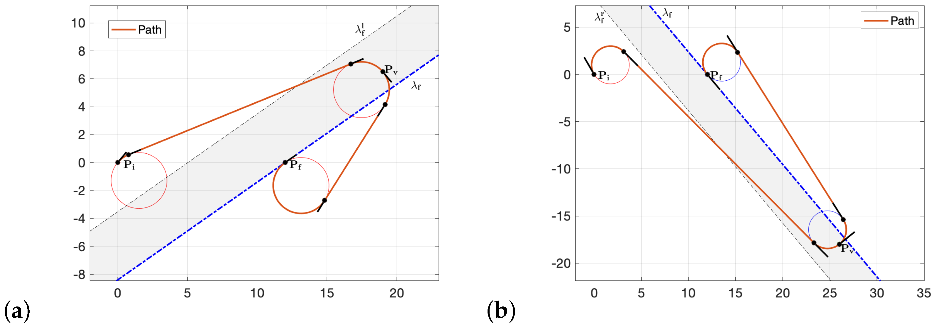
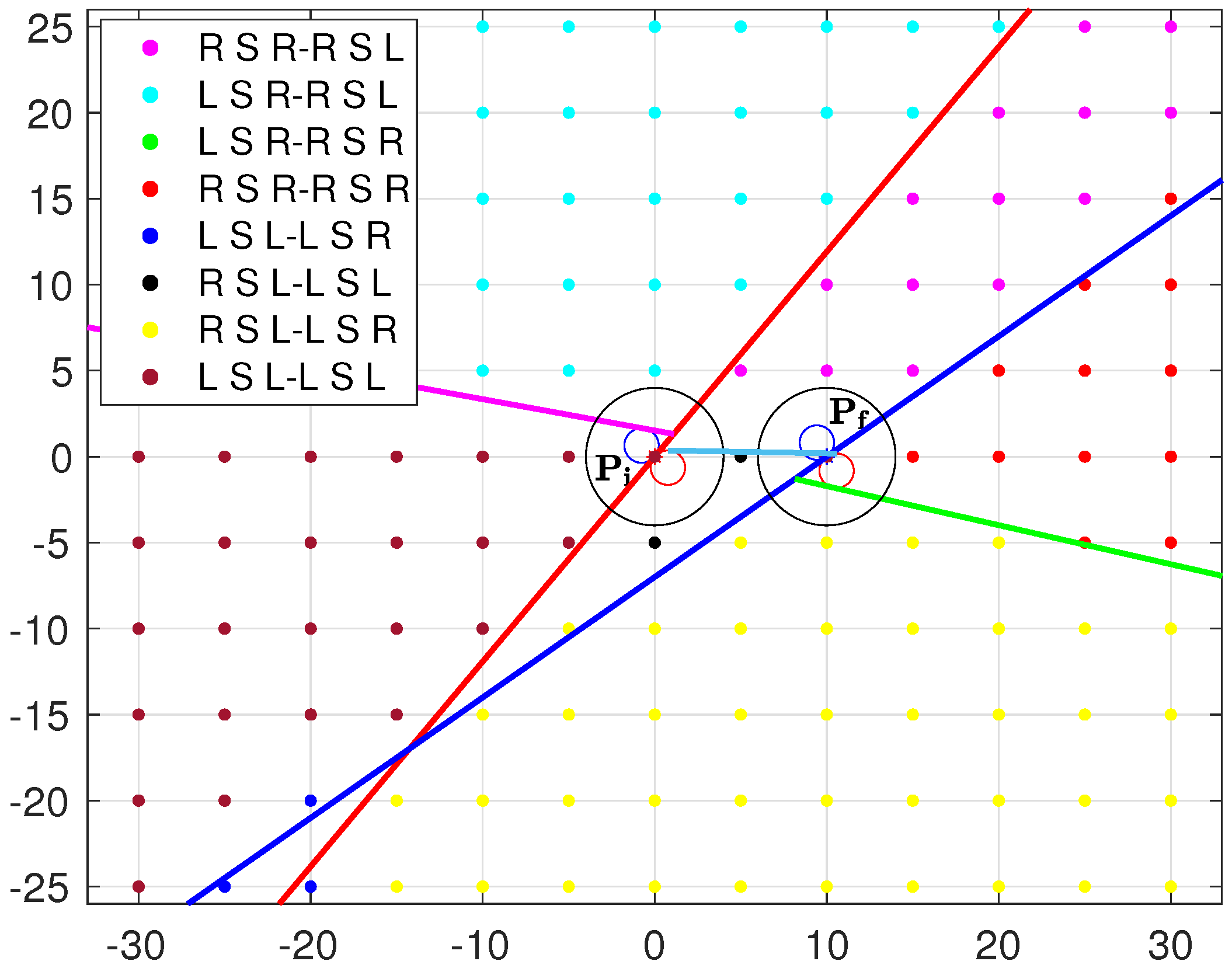
3. Classification Rules

Our goal is to build a partition of the Cartesian plane as the one illustrated in Figure 6, which represents a partition for the classification of a 3PDP with distance $d=15$ between the initial and final points, and initial and final orientation, ${\theta }_i$ and ${\theta }_f$ on quadrant I. Referring to this partition, given any via point ${\mathit{P}}_v$, it is possible to immediately deduce the optimal path type by simply identifying the region to which it belongs. Consider the via point ${\mathit{P}}_v=(-10,15)$ in Figure 6: it lies in the region classified as $LSR-RSL$. Indeed, by computing the optimal path type with the conventional methods available in the literature, the resulting path reported in Figure 6 is actually an $LSR-RSL$ path type.

Figure 6. Classification of $CSC-CSC$ paths with ${\theta }_i$ and ${\theta }_f$ on quadrant I: example of partition.

In general, to build a complete path type classification, we need to select the optimal turning directions on the three points of interest, i.e., the curvature at the initial point $C_{initial}$, the curvature at the final point $C_{final}$, and the curvature at the via point $C_{viaPoint}$.

3.1. Curvature at the Initial Point

As a first step, draw a straight line starting from ${\mathit{P}}_i$ with orientation ${\theta }_i$, and denote it as ${\lambda }_i$, as in Figure 6. A first simple intuitive idea that we explore is that, if the via point ${\mathit{P}}_v$ is on the left of ${\lambda }_i$, then the first turning direction is necessarily on the left, while if ${\mathit{P}}_v$ is on the right with respect to ${\lambda }_i$, then the optimal path turn is on the right (see Figure 7).

Figure 7. Optimal paths with $P_v$ on the right and on the left of the straight line ${\lambda }_i$.

However, a deeper insight into this point shows that there are some points close to ${\lambda }_i$ that do not follow the above logic, and the reason is subtle. Without loss of generality, consider the example reported in Figure 8 where the via point ${\mathit{P}}_v$ is on the right and near ${\lambda }_i$. In such a case, the optimal path type has the first turn on the left instead of on the right.

Figure 8. The example with $P_v$ is on the right of ${\lambda }_i$ and first turn on the left.

It is possible to clarify the reason for this phenomenon, which is the following. The orientation at ${\mathit{P}}_v$ requires a right turn, so if the initial turning point (${\mathit{P}}_{v_{q_1}}$ in Figure 8) is on the opposite side of ${\mathit{P}}_v$ with respect to ${\lambda }_i$, then the initial turn is on the left.

In order to correctly identify and manage this phenomenon, two different approaches can be adopted: an analytical approach and a heuristic one.

3.1.1. Analytical Approach

As an illustrative example, we still consider a case with ${\theta }_i$ and ${\theta }_f$ on quadrant I as in Figure 8.

The analytical approach exploits the optimal condition, Equation (2). Following this approach, the main goal is to derive the exact boundary, denoted as ${\mathcal{I}}_i$ hereafter, between paths that differ in curvature at the initial point, i.e., $RSR-RSL$ and $LSR-RSL$ for the example under investigation. Analytically, the boundary of the two regions $RSR-RSL$ and $LSR-RSL$ is defined by those points ${\mathit{P}}_v$ for which the $RSR-RSL$ and $LSR-RSL$ paths have the same lengths, i.e.,

$$L_{1_{RSR}}\left({\theta }_v\right)+L_{2_{RSL}}\left({\theta }_v\right)=L_{1_{LSR}}\left({\theta }_v\right)+L_{2_{RSL}}\left({\theta }_v\right).$$

(4)

From a geometrical point of view, given that the second elementary Dubins paths between the via point and the final configuration are the same ($RSL$ type of length $L_{2_{RSL}}$), the two types of paths $RSR-RSL$ and $LSR-RSL$ have the same lengths when the length of the straight line segment $p_1$ associated to the first elementary Dubins path is the same, namely,

$$L_{1_{RSR}}\left({\theta }_v\right)=L_{1_{LSR}}\left({\theta }_v\right).$$

For the $RSR$ path, the segment $p_1$ is given by the common external tangent $r_{rr}^{e+}$ between the circles ${\mathcal{C}}_{i_r}$ and ${\mathcal{C}}_{v_r}$; while for the $LSR$ path, the segment $p_1$ is given by the common cross tangent $r_{lr}^{c-}$ between the circles ${\mathcal{C}}_{i_l}$ and ${\mathcal{C}}_{v_r}$ (see tangents in the Figure 9). As a consequence, the optimality condition in Equation (4) is as follows:

$$r_{rr}^{e+}\equiv r_{lr}^{c-}.$$

(5)

Figure 9. Geometric representation of the optimality condition in (5).

This happens when the circle ${\mathcal{C}}_{v_r}$ is tangential to the line ${\lambda }_i$; in this case, the point ${\mathit{P}}_{v_{q_1}}\in {\lambda }_i$. As a consequence, the first arc $t_1$ has zero length (i.e., $t_1=0$) and the two paths collapse in a path of type $SR-RSL$. Refer to Figure 9 for a clear geometric representation of the optimality condition.

In order to actually find the locus of via points that correspond to such an optimal $SR-RSL$ path type, the optimality condition given by Lemma 1 for the $SR-RSL$ path should be verified, that is

$${\mathbf{v}}^{\top }{\mathbf{v}}_{{\theta }_v}=0,$$

(6)

where        

$$\begin{array}{ccc}\hfill & & \mathbf{v}={\mathbf{e}}_{v_i}+{\mathbf{e}}_{v_f},\hfill \end{array}$$

(7)

$${\mathbf{e}}_{v_i}={\displaystyle \frac{{\mathbf{c}}_{v_r}-{\mathbf{c}}_{i_r}}{|{\mathbf{c}}_{v_r}-{\mathbf{c}}_{i_r}|}}={[cos\left({\theta }_i\right)sin\left({\theta }_i\right)]}^{\top },$$

(8)

$$\begin{array}{ccc}& & {\mathbf{e}}_{v_f}=\mathit{R}\left(\gamma \right){\displaystyle \frac{{\mathbf{c}}_{v_r}-{\mathbf{c}}_{f_l}}{|{\mathbf{c}}_{v_r}-{\mathbf{c}}_{f_l}|}},\mathrm{with}\gamma ={sin}^{-1}\left({\displaystyle \frac{2{\mathrm{\Omega }}^{-1}}{|{\mathbf{c}}_{v_r}-{\mathbf{c}}_{f_l}|}}\right),\hfill \end{array}$$

(9)

$$\begin{array}{ccc}\hfill & & {\mathbf{v}}_{{\theta }_v}={[-(y_v-y_{v_r}),(x_v-x_{v_r})]}^{\top },\hfill \end{array}$$

(10)

and $\mathit{R}\left(\gamma \right)\in {\mathbb{R}}^2$ is the standard rotation matrix. We also recall that in the intersection domain, the first arc vanishes, i.e., $t_1=0$, the direction of ${\mathbf{e}}_{v_i}$ coincides with the initial orientation ${\theta }_i$, and the first elementary Dubins path reduces to an $SR$-type path (see Figure 10).

Figure 10. Optimal $SR-RSL$ path ($t_1=0$).

As a result, the centers ${\mathbf{c}}_{v_r}=(x_{v_r},y_{v_r})$ lie on the line ${\lambda }_i^{r^{\prime }}$, which is a line parallel to ${\lambda }_i$ and distant ${\mathrm{\Omega }}^{-1}$ to its right, so that the optimal right via point circle ${\mathcal{C}}_{v_r}$ is a circle passing through the via point and tangent to the line ${\lambda }_i$. The versor ${\mathbf{e}}_{v_f}$ identifies the direction of the cross tangent of the circles ${\mathcal{C}}_{v_r}$ and ${\mathcal{C}}_{f_l}$. Hence, the points of the curve ${\mathcal{I}}_i$ can be obtained by adding at each center ${\mathbf{c}}_{v_r}$ the versor ${\mathbf{e}}_v$ (i.e., the versor in the direction of $\mathbf{v}={\mathbf{e}}_{v_i}+{\mathbf{e}}_{v_f}$ ) multiplied by ${\mathrm{\Omega }}^{-1}$.

Summarizing, from an analytical point of view, we have one Equation (6) with two variables: $x_{v_r}$ and $y_{v_r}$. We can solve it by taking one variable as a parameter. The analytical result is a curve ${\mathcal{I}}_i$ that admits as asymptote the line ${\lambda }_i^{r^{\prime }}$ (see Figure 11).

Figure 11. Frontier between $RSR-RSL$ and $LSR-RSL$ for ${\theta }_i$ and ${\theta }_f$ on quadrant I: (a) radius of the limiting circle ${\mathrm{\Omega }}^{-1}=1$, (b) radius of the limiting circle ${\mathrm{\Omega }}^{-1}=2$.

Figure 11a,b show the curve ${\mathcal{I}}_i$, i.e., the frontier between the regions $RSR-RSL$ and $LSR-RSL$ for ${\theta }_i$ and ${\theta }_f$ on quadrant I, for different values of the maximum turning radius: ${\mathrm{\Omega }}^{-1}=1$ and ${\mathrm{\Omega }}^{-1}=2$, respectively. At this point, we can formulate the classification rules for identifying the curvature at the initial point $C_{initial}$ as given in Algorithm 1.

Algorithm 1 Initial curvature-analytical approach

Require: ${\mathbf{q}}_i$, ${\mathbf{q}}_f$, ${\mathit{P}}_v$ Ensure: $C_{initial}$  compute curve ${\mathcal{I}}_i$ from Equation (6)  if ${\mathit{P}}_v\in {\pi }_{{\mathcal{I}}_i}^r$ then   $C_{initial}=R$  else   $C_{initial}=L$  end if

It is worth noting that the derivation of the exact curve ${\mathcal{I}}_i$ could be demanding from a computational point of view (it requires solving nonlinear equations), so when the available computational load is limited, it could be preferable to resort to a heuristic approach—which is simpler, more efficient, and practical—as detailed below.

3.1.2. Heuristic Approach

A heuristic solution to determine the initial curvature for points close to ${\lambda }_i$ is still based on the fact that the boundary is associated with paths having ${\mathit{P}}_{v_{q_1}}\in {\lambda }_i$ (hence, the first arc of zero length $t_1=0$ for the example under investigation). As a result, the maximum distance between the point ${\mathit{P}}_v$ on the frontier and the line ${\lambda }_i$ is $2{\mathrm{\Omega }}^{-1}$. It is obtained by imposing that the optimal circle at the via point is tangential to the line ${\lambda }_i$, or equivalently, for the example under investigation, the first arc of zero length, i.e., $t_1=0$. This allows us to consider a region between ${\lambda }_i$ and the line ${\lambda }_i^r$ (${\lambda }_i^r$ being a line parallel to ${\lambda }_i$ on its right and distant $2{\mathrm{\Omega }}^{-1}$) where the investigation should consider two types of potentially optimal paths (either starting with L turn or R turn). This region is highlighted in gray in Figure 11a. A practical way to manage the points in this region is to test both possibilities, which is simpler and less demanding.

The above result is still valid for ${\theta }_i$ on quadrant II, whereas symmetric considerations hold for ${\theta }_i$ on quadrants III and IV. In the latter cases, the region that requires us to test both possibilities is the area between ${\lambda }_i$ and the line ${\lambda }_i^l$, namely, a line parallel to ${\lambda }_i$ on its left and distant $2{\mathrm{\Omega }}^{-1}$ (see Figure 12).

Figure 12. Example of optimal path with ${\theta }_i$ on quadrant III where ${\mathit{P}}_v$ is on the left of ${\lambda }_i$ but the optimal initial turn is right.

The resulting classification rules for identifying the curvature at the initial point are summarized in Algorithm 2. The output of the algorithm is the turning direction at the initial point: “R” for a right turn, “L” for a left turn, and “C” for a generic curvature on the left or on the right (that is, when both should be tested). It is worth noticing that in the boundary between the quadrants $Q_I$-$Q_{IV}$ and $Q_{II}$-$Q_{III}$ (i.e., ${\theta }_i\in \{0,\pi \}$), a more conservative region is considered, that is, the union of the candidate regions associated with both cases.

Algorithm 2 Initial curvature-heuristic approach

Require: ${\mathbf{q}}_i$, ${\mathit{P}}_v$ Ensure: $C_{initial}$  $C_{initial}=C$  if ${\theta }_i\in (0,\pi )$ (${\theta }_i\in \{Q_I,Q_{II}\}$) then   if ${\mathit{P}}_v\in {\pi }_{{\lambda }_i}^l$ then    $C_{initial}=L$    else if ${\mathit{P}}_v\in {\pi }_{{\lambda }_i^r}^r$ then    $C_{initial}=R$   end if  else if ${\theta }_i\in (\pi ,2\pi )$ (${\theta }_i\in \{Q_{III},Q_{IV}\}$) then   if ${\mathit{P}}_v\in {\pi }_{{\lambda }_i^l}^l$ then    $C_{initial}=L$    else if ${\mathit{P}}_v\in {\pi }_{{\lambda }_i}^r$ then    $C_{initial}=R$   end if   else if ${\theta }_i\in \{0,\pi \}$ then   if ${\mathit{P}}_v\in {\pi }_{{\lambda }_i^l}^l$ then    $C_{initial}=L$    else if ${\mathit{P}}_v\in {\pi }_{{\lambda }_i^r}^r$ then    $C_{initial}=R$   end if  end if

3.2. Curvature at the Final Point

Similar considerations hold for the optimal turning direction at the final point. Draw the line ${\lambda }_f$ passing through ${\mathit{P}}_f=(x_f,y_f)$ with orientation ${\theta }_f$. If the via point ${\mathit{P}}_v$ is on the left of ${\lambda }_f$, then the last turning direction is on the left, while if ${\mathit{P}}_v$ is on its right, the optimal path type is associated with a right last turn. An example is illustrated in Figure 13.

Figure 13. Example of optimal paths where ${\mathit{P}}_v$ is on the right and on the left of the straight line ${\lambda }_f$.

Also, in this case, if the via point ${\mathit{P}}_v$ lies in the neighborhood of ${\lambda }_f$, an analogous phenomenon to the one described in Section 3.1 happens.

Consider Figure 14a where the via point ${\mathit{P}}_v$ is near ${\lambda }_f$ and on its left. In such a case, the optimal path type has the last turn on the right (instead of on the left). Again, it is possible to manage this phenomenon by adopting an analytical approach or a heuristic one.

Figure 14. (a) Example of a situation with ${\theta }_f$ on quadrant I. (b) Example of situation with ${\theta }_f$ on quadrant IV.

3.2.1. Analytical Approach

As an illustrative example, we still take a case with ${\theta }_i$ and ${\theta }_f$ on quadrant I as shown in Figure 6. We can resort to an analytical approach, similar to the one presented in the previous section, to derive the exact frontier that differs for a curvature at the final point, e.g., $RSL-LSL$ and $RSL-LSR$ for the example at hand. This partition domain is given by the via points where the two types of paths have the same length. Similar to the case of the initial turning direction, such a condition is satisfied when the turning operation at ${\mathit{P}}_v$ has its end point ${\mathit{P}}_{v_{t2}}$ on the line ${\lambda }_f$, i.e., ${\mathit{P}}_{v_{t2}}\in {\lambda }_f$, so that the two paths collapse in a path of type $RSL-LS$, and the last arc $q_2$ has zero length (i.e., $q_2=0$). In order to actually find the locus of via points corresponding to such an optimal $RSL-LS$ path type, the optimality condition given by Lemma 1 for the $RSL-LS$ path is as follows:

$${\mathbf{v}}^{\top }{\mathbf{v}}_{{\theta }_v}=0,$$

(11)

where        

$$\begin{array}{ccc}\hfill & & \mathbf{v}={\mathbf{e}}_{v_i}+{\mathbf{e}}_{v_f}\hfill \end{array}$$

(12)

$$\begin{array}{ccc}\hfill & & {\mathbf{e}}_{v_i}=\mathit{R}\left(\gamma \right){\displaystyle \frac{{\mathbf{c}}_{v_r}-{\mathbf{c}}_{i_r}}{|{\mathbf{c}}_{v_r}-{\mathbf{c}}_{i_r}|}},\mathrm{with}\gamma ={sin}^{-1}{\displaystyle \frac{2{\mathrm{\Omega }}^{-1}}{|{\mathbf{c}}_{v_r}-{\mathbf{c}}_{i_r}|}},\hfill \end{array}$$

(13)

$$\begin{array}{ccc}& & {\mathbf{e}}_{v_f}={\displaystyle \frac{{\mathbf{c}}_{v_r}-{\mathbf{c}}_{f_l}}{|{\mathbf{c}}_{v_r}-{\mathbf{c}}_{f_l}|}}={[cos\left({\theta }_f\right)sin\left({\theta }_f\right)]}^{\top },\hfill \end{array}$$

(14)

$$\begin{array}{ccc}\hfill & & {\mathbf{v}}_{{\theta }_v}={[-(y_v-y_{v_r}),(x_v-x_{v_r})]}^{\top }.\hfill \end{array}$$

(15)

Again, in the intersection domain, the last arc vanishes, i.e., $q_2=0$, so that the direction of ${\mathbf{e}}_{v_f}$ coincides with the final orientation ${\theta }_f$. As a result, the centers ${\mathbf{c}}_{v_l}=(x_{v_l},y_{v_l})$ lie on the line ${\lambda }_f^{l^{\prime }}$, namely, a line parallel to ${\lambda }_f$ on its left and distant ${\mathrm{\Omega }}^{-1}$, so that the optimal left via point circle ${\mathcal{C}}_{v_l}$ is a circle passing through the via point and tangent to the line ${\lambda }_f$.

Therefore, from an analytical point of view, Equation (11) with the two variables $x_{v_l}$ and $y_{v_l}$ provides the solution. The analytical result is a curve ${\mathcal{I}}_f$ that admits as asymptote the line ${\lambda }_f^{l^{\prime }}$. The classification rules for identifying the curvature at the final point $C_{final}$ are given in Algorithm 3.

Algorithm 3 Final curvature-analytical approach

Require: ${\mathbf{q}}_i$, ${\mathbf{q}}_f$, ${\mathit{P}}_v$ Ensure: $C_{final}$  compute curve ${\mathcal{I}}_f$ from Equation (11)  if  ${\mathit{P}}_v\in {\pi }_{{\mathcal{I}}_f}^r$ then   $C_{final}=R$  else   $C_{final}=L$  end if

3.2.2. Heuristic Approach

The heuristic solution to determine the final curvature for points close to ${\lambda }_f$ is based on the fact that the boundary is associated with paths having the point ${\mathit{P}}_{v_{t_2}}\in {\lambda }_f$ (hence, the last arc of zero length $q_2=0$ for the example under investigation). As a consequence, the maximum distance between the point ${\mathit{P}}_v$ on the frontier and the line ${\lambda }_f$ is $2{\mathrm{\Omega }}^{-1}$. Again, it is possible to consider a region between ${\lambda }_f$ and the line ${\lambda }_f^l$ parallel to ${\lambda }_f$ on its left and distant $2{\mathrm{\Omega }}^{-1}$, so that a way to manage the points in this region is to test both possibilities. This region is highlighted in gray in Figure 14a. Outside this region, the curvature can be immediately obtained following a simple classification rule.

This result is valid for ${\theta }_f\in \{Q_I,Q_{II}\}$, whereas when the final orientation ${\theta }_f\in \{Q_{III},Q_{IV}\},$ symmetric considerations hold, so the line ${\lambda }_f^r$ parallel to ${\lambda }_f$ on its right should be considered, as shown in Figure 14b. The resulting classification rules for identifying the curvature at the final point are summarized in Algorithm 4.

3.3. Curvature at the via Point

In this subsection, we complete the classification scheme with the identification of the turning direction at the via point. We separately consider the cases of paths with “zero” and “non-zero” curvature at the via point.

3.3.1. Paths with Zero Curvature at the via Point

We start with the consideration that paths with zero curvature at the via point ${\mathit{P}}_v$ are all and only those having the via point ${\mathit{P}}_v$ on the length-optimal Dubins path between ${\mathit{P}}_i$ and ${\mathit{P}}_f$ (see, for example, the light blue line in Figure 15). We denote such an oriented segment (starting from the initial optimal circle and ending at the final optimal circle) as ${\lambda }_0$ from now on (its orientation is defined as positive from ${\mathit{P}}_i$ to ${\mathit{P}}_f$). The importance of the segment ${\lambda }_0$ is that all the via points on the left of ${\lambda }_0$ ($P_v\in {\pi }_{{\lambda }_0}^l$) are associated with paths with a right-turn direction at the via point $C_{viaPoint}=R$ (hence of type $CSR-RSC$), and those on the right ($P_v\in {\pi }_{{\lambda }_0}^r$) are paths with a left-turn direction at $C_{viaPoint}=L$, i.e., $CSL-LSC$ paths.

Figure 15. The vectors ${\mathbf{v}}_i$ and ${\mathbf{v}}_f$ for a path with zero curvature at the via point.

In order to derive the conditions to identify paths with zero curvature at the via point, we start from the property of the three-point Dubins path provided in Lemma 1; see Figure 5.

Algorithm 4 Final curvature-heuristic approach

Require: ${\mathbf{q}}_f$, ${\mathit{P}}_v$ Ensure: $C_{final}$   $C_{final}=C$  if ${\theta }_f\in (0,\pi )$ (${\theta }_f\in \{Q_I,Q_{II}\}$) then   if ${\mathit{P}}_v\in {\pi }_{{\lambda }_f^l}^l$ then    $C_{final}=L$    else if ${\mathit{P}}_v\in {\pi }_{{\lambda }_f}^r$ then    $C_{final}=R$   end if  else if ${\theta }_f\in (\pi ,2\pi )$ (${\theta }_f\in \{Q_{III},Q_{IV}\}$) then   if ${\mathit{P}}_v\in {\pi }_{{\lambda }_f}^l$ then    $C_{final}=L$    else if ${\mathit{P}}_v\in {\pi }_{{\lambda }_f^r}^r$ then    $C_{final}=R$   end if  else if ${\theta }_f\in \{0,\pi \}$ then   if ${\mathit{P}}_v\in {\pi }_{{\lambda }_f^l}^l$ then    $C_{final}=L$    else if ${\mathit{P}}_v\in {\pi }_{{\lambda }_f^r}^r$ then    $C_{final}=R$   end if  end if

According to Lemma 1, for a shortest path of type $CSC-CSC$, the bisector $\mathbf{v}$ between ${\mathbf{v}}_i$ and ${\mathbf{v}}_f$ is collinear with ${\mathbf{v}}_v$ (see Figure 5) and consequently orthogonal to ${\mathbf{v}}_{{\theta }_v}$, leading to the optimality condition ${\mathbf{v}}^{\top }{\mathbf{v}}_{{\theta }_v}=\mathbf{0}$.

The condition of zero curvature at the via point is verified when the bisector $\mathbf{v}$ is the null vector, i.e., $\mathbf{v}=\mathbf{0}$, which is when

$${\mathbf{v}}_i=-{\mathbf{v}}_f.$$

In this condition, ${\mathbf{v}}_i$ and ${\mathbf{v}}_f$ lie on the common tangent between the circles associated with the optimal initial and final turns.

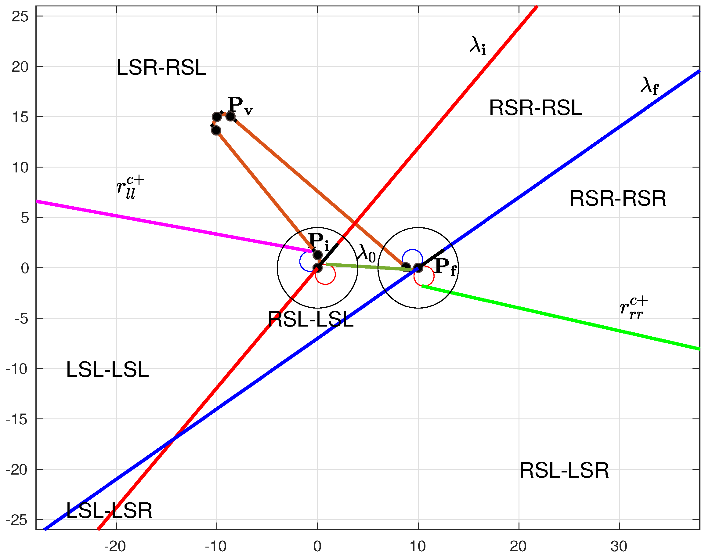
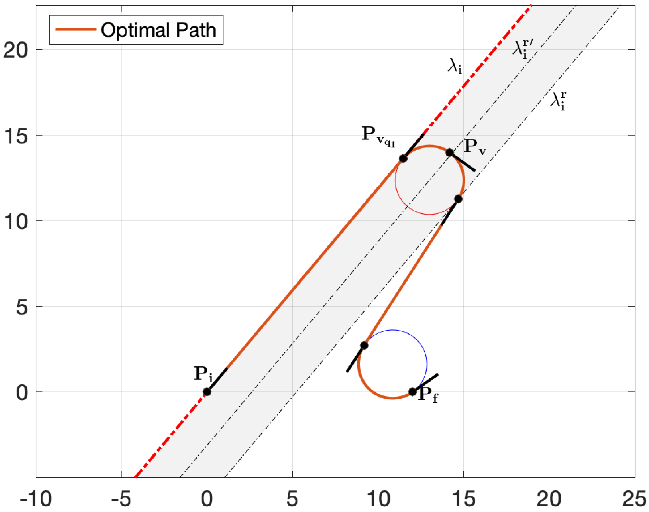
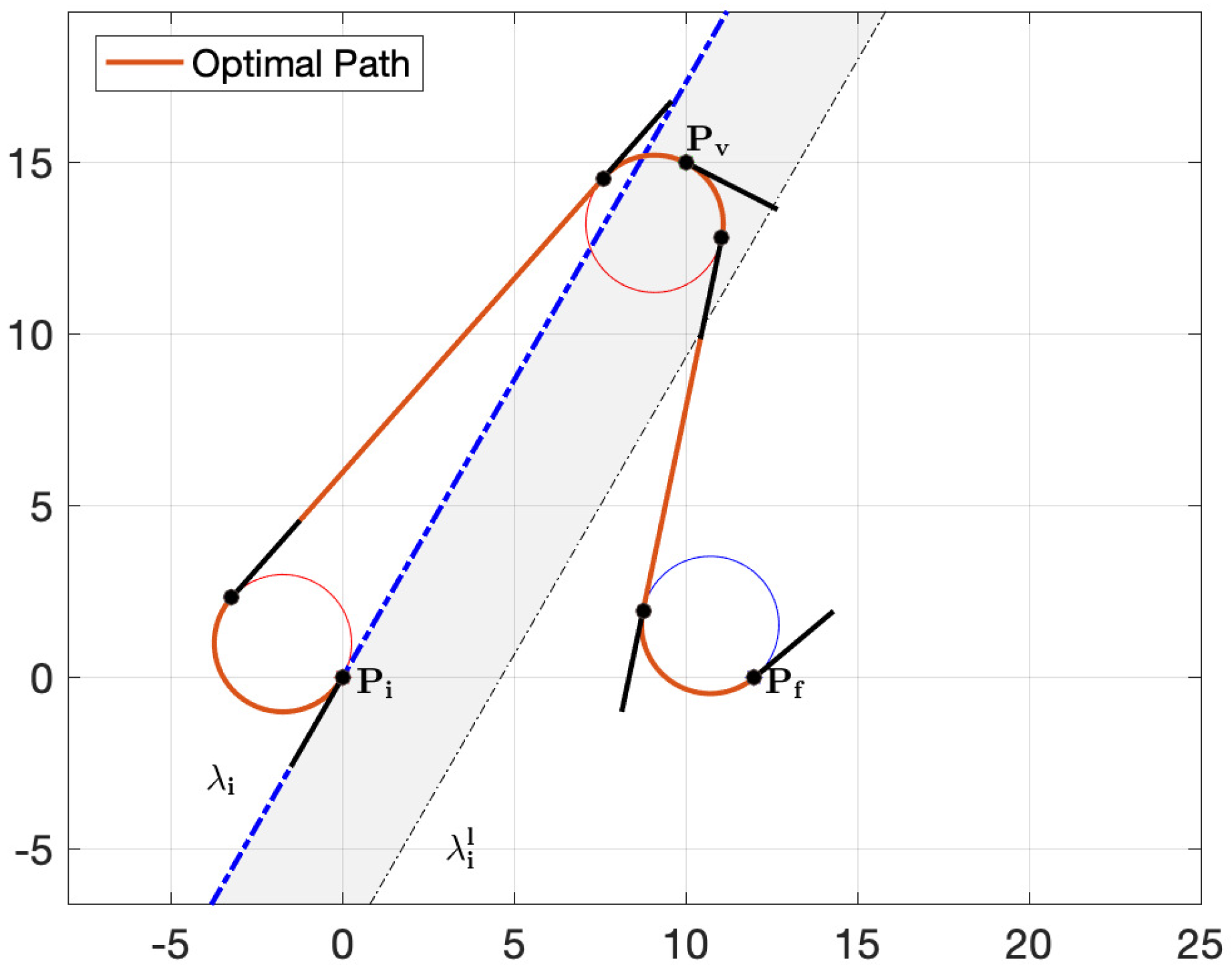
3.3.2. Paths with Non-Zero Curvature at the via Point

As for paths with non-zero curvature at the via point, it is possible to derive a condition useful to identify regions that differ only for the curvature at the via point. Indeed, the boundary of these regions is made of all points ${\mathit{P}}_v$ for which the two types of path have the same length. In order to exploit such idea, consider again the example of a partition of the Cartesian plane in Figure 16.

Figure 16. Example of plane partitioning for classification. Three different regions are highlighted in the Cartesian plane.

Note that there are distinct areas where the optimal path type has a different curvature at the via point. It is useful to define an appropriate notation to separate these areas:

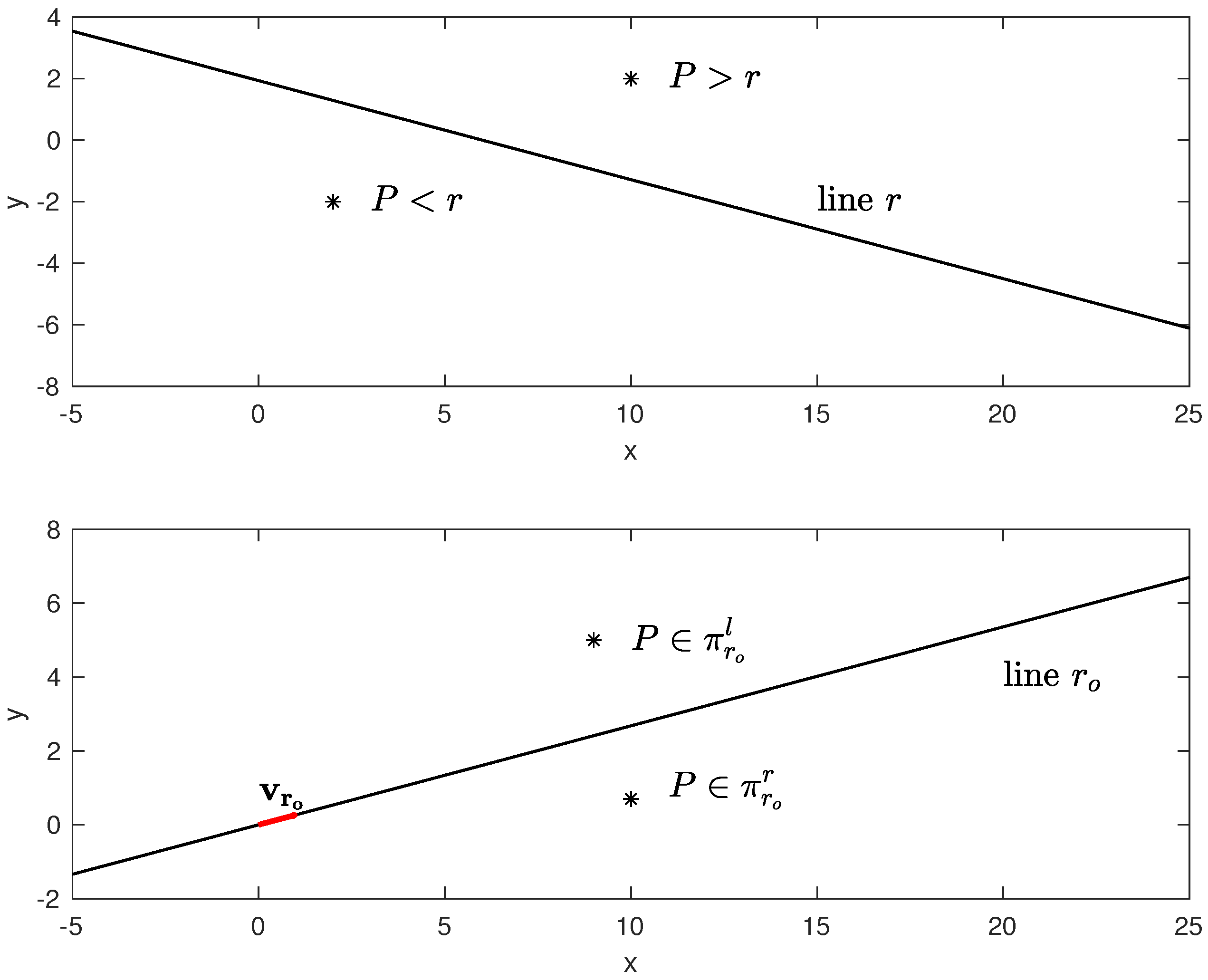
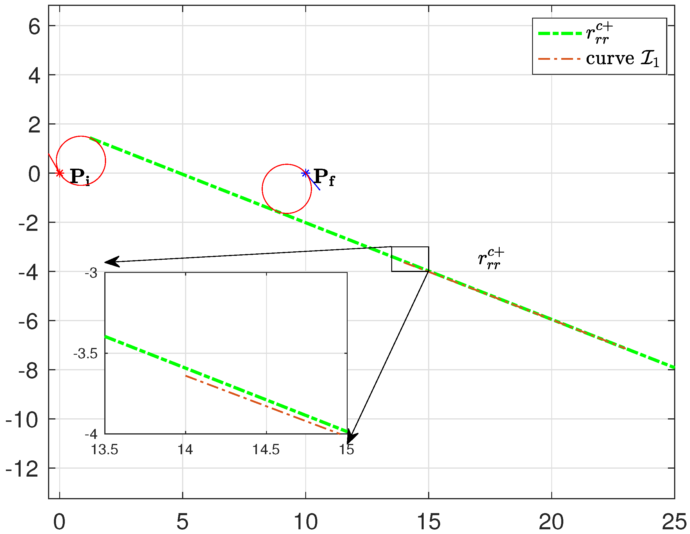
• ${\mathit{P}}_v\in$ Region 1: boundary $RSR-RSR/RSL-LSR$ denoted as ${\mathcal{I}}_1$
• ${\mathit{P}}_v\in$ Region 0: boundary $RSR-RSL/RSL-LSL$ denoted as ${\mathcal{I}}_0$
• ${\mathit{P}}_v\in$ Region 2: boundary $LSR-RSL/LSL-LSL$ denoted as ${\mathcal{I}}_2$

In the following subsection, we derive the exact frontier between paths with different curvatures at the via point, either referring to an analytical one or to the heuristic one.

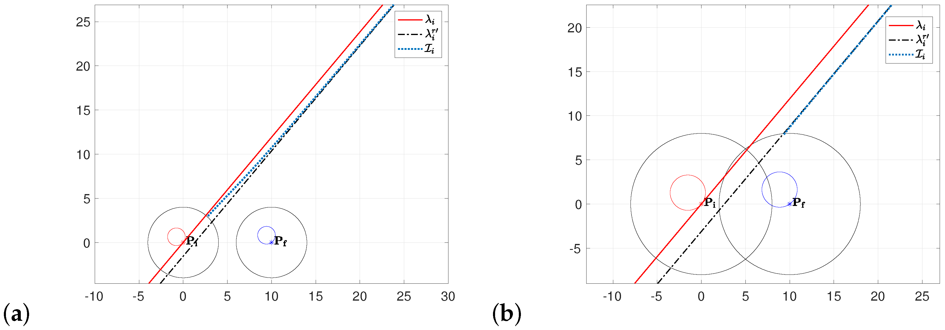
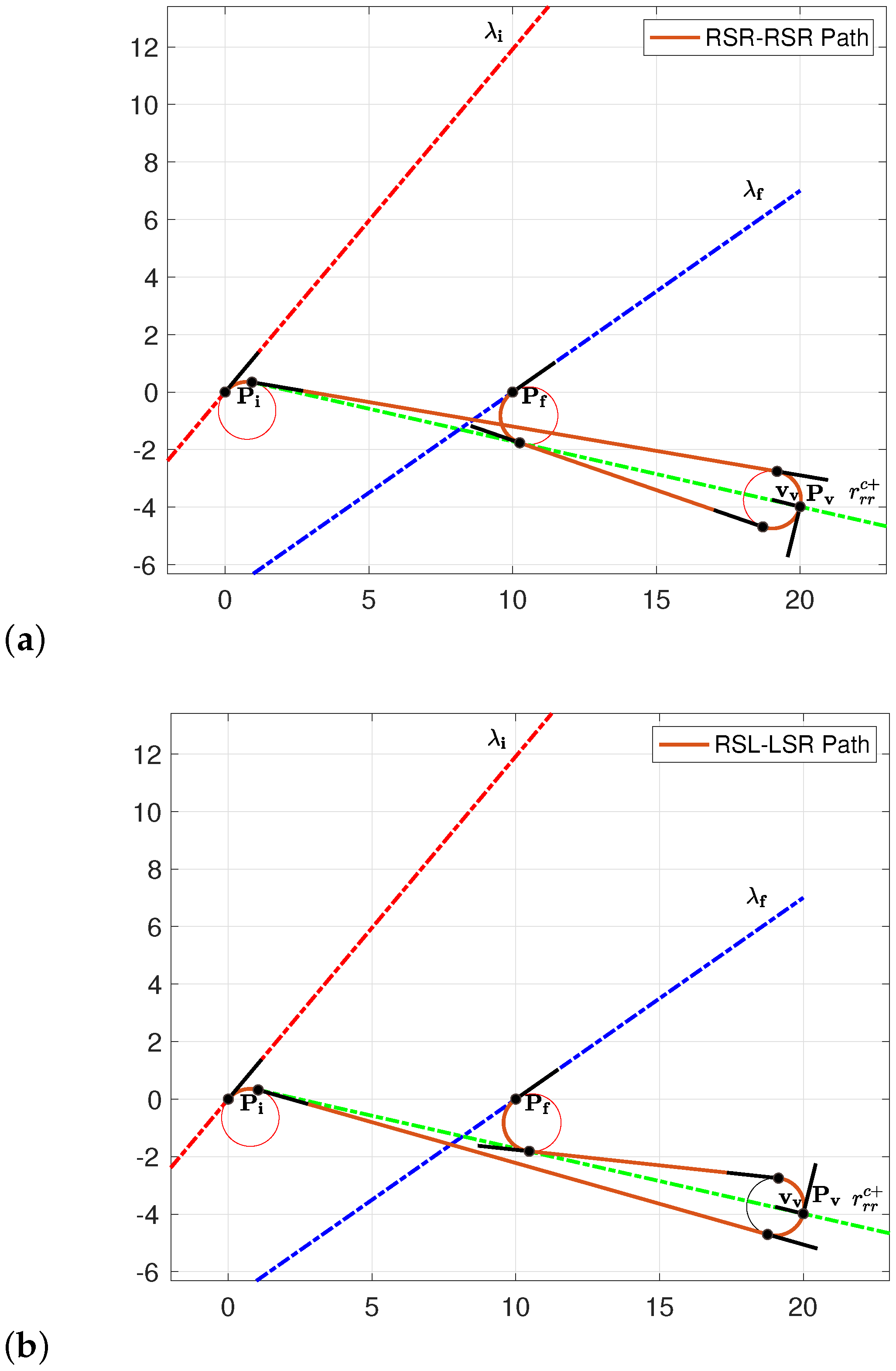
3.3.3. Derivation of the Boundary between Domains with Different Curvatures at the via Point

Consider the boundary $RSR-RSR/RSL-LSR$ first. A clear representation of this case is illustrated in Figure 17 where ${\theta }_i$ and ${\theta }_f$ are on quadrant I.

Figure 17. Example of paths with equal lengths for a case with ${\theta }_i$ and ${\theta }_f$ on quadrant I, and ${\mathit{P}}_v$ on $r_{rr}^{c+}$: (a) $RSR-RSR$ path type, (b) $RSL-LSR$ path type.

The $RSR-RSR$ and $RSL-LSR$ path types associated with the via point ${\mathit{P}}_v$ in Figure 17 have the same length; they differ only in the curvature at the via point. The optimal direction ${\theta }_v^R$ associated with the $RSR-RSR$ path type and ${\theta }_v^L$ associated with the $RSL-LSR$ path type have opposite directions, so that

$${\theta }_v^R={\theta }_v^L+\pi .$$

(16)

Therefore, they are both orthogonal to the vector ${\mathbf{v}}_v$, having denoted with ${\mathbf{v}}_v$ the vector connecting the center of the circle associated with the optimal heading and the via point ${\mathit{P}}_v$.

In order to analytically derive the partition boundary between the $RSR-RSR$ and $RSL-LSR$ path types, the first condition to be verified is that the two types of paths should have the same length, so we have the following:

$$L_{1_{RSR-RSR}}\left({\theta }_v^R\right)+L_{2_{RSR-RSR}}\left({\theta }_v^R\right)=L_{1_{RSL-LSR}}\left({\theta }_v^L\right)+L_{2_{RSL-LSR}}\left({\theta }_v^L\right),$$

which results in the following equation:

$$\begin{array}{c}\sqrt{{(x_{ir}-x_{vr})}^2+{(y_{ir}-y_{vr})}^2}+\sqrt{{(x_{vr}-x_{fr})}^2+{(y_{vr}-y_{fr})}^2}\\ =\sqrt{{(x_{ir}-x_{vl})}^2+{(y_{ir}-y_{vl})}^2-{\left({\displaystyle \frac{2}{\mathrm{\Omega }}}\right)}^2}+\sqrt{{(x_{vl}-x_{fr})}^2+{(y_{vl}-y_{fr})}^2-{\left({\displaystyle \frac{2}{\mathrm{\Omega }}}\right)}^2}.\end{array}$$

(17)

From the optimality condition (Lemma 1) for the $RSR-RSR$ and $RSL-LSR$ paths, the following condition must be verified:

$$\begin{array}{c}\hfill {({\mathbf{e}}_i^R+{\mathbf{e}}_f^R)}^{\top }{\mathbf{v}}_{{\theta }_v^R}=0,\end{array}$$

(18)

$$\begin{array}{c}\hfill {({\mathbf{e}}_i^L+{\mathbf{e}}_f^L)}^{\top }{\mathbf{v}}_{{\theta }_v^L}=0\end{array}$$

(19)

where the superscripts R and L denote that the versor ${\mathbf{e}}_i$ or ${\mathbf{e}}_f$ refers to the path with right and left curvatures at the via point, respectively. This leads to a system of three equations (Equations (17)–(19)) with four variables (${\mathit{P}}_v=(x_v,y_v),{\theta }_v^R,{\theta }_v^L$):

$$\begin{array}{ccc}\hfill {\mathbf{e}}_i^R& =& {\displaystyle \frac{{\mathbf{c}}_{vr}-{\mathbf{c}}_{ir}}{|{\mathbf{c}}_{vr}-{\mathbf{c}}_{ir}|}}\hfill \end{array}$$

(20)

$$\begin{array}{ccc}\hfill {\mathbf{e}}_f^R& =& {\displaystyle \frac{{\mathbf{c}}_{vr}-{\mathbf{c}}_{fr}}{|{\mathbf{c}}_{vr}-{\mathbf{c}}_{fr}|}}\hfill \end{array}$$

(21)

$$\begin{array}{ccc}\hfill {\mathbf{v}}_{{\theta }_v^R}& =& {[-(y_v-y_{vr}),(x_v-x_{vr})]}^{\top }\hfill \end{array}$$

(22)

$$\begin{array}{ccc}\hfill {\mathbf{e}}_i^L& =& \mathit{R}\left({\gamma }_i\right){\displaystyle \frac{{\mathbf{c}}_{vl}-{\mathbf{c}}_{ir}}{|{\mathbf{c}}_{vl}-{\mathbf{c}}_{ir}|}}\mathrm{with} {\gamma }_i={sin}^{-1}\left({\displaystyle \frac{2{\mathrm{\Omega }}^{-1}}{|{\mathbf{c}}_{vl}-{\mathbf{c}}_{ir}|}}\right)\hfill \end{array}$$

(23)

$$\begin{array}{ccc}\hfill {\mathbf{e}}_f^L& =& \mathit{R}\left({\gamma }_f\right){\displaystyle \frac{{\mathbf{c}}_{vl}-{\mathbf{c}}_{fr}}{|{\mathbf{c}}_{vl}-{\mathbf{c}}_{fr}|}}\mathrm{with} {\gamma }_f={sin}^{-1}\left({\displaystyle \frac{2{\mathrm{\Omega }}^{-1}}{|{\mathbf{c}}_{vl}-{\mathbf{c}}_{fr}|}}\right)\hfill \end{array}$$

(24)

$$\begin{array}{ccc}\hfill {\mathbf{v}}_{{\theta }_v^L}& =& {[-(y_v-y_{vl}),(x_v-x_{vl})]}^{\top }\hfill \end{array}$$

(25)

$$\begin{array}{ccc}\hfill {\mathbf{c}}_{vr}& =& {[x_v+{\mathrm{\Omega }}^{-1}sin\left({\theta }_v^R\right),y_v-{\mathrm{\Omega }}^{-1}cos\left({\theta }_v^R\right)]}^{\top }\hfill \end{array}$$

(26)

$$\begin{array}{ccc}\hfill {\mathbf{c}}_{vl}& =& {[x_v-{\mathrm{\Omega }}^{-1}sin\left({\theta }_v^L\right),y_v+{\mathrm{\Omega }}^{-1}cos\left({\theta }_v^L\right)]}^{\top }.\hfill \end{array}$$

(27)

The analytical result, obtained solving the above system of equations, is a curve ${\mathcal{I}}_1$ quite close to the common tangent (superior cross tangent) $r_{rr}^{c+}$ between the circles associated with the optimal initial and final turns as shown in Figure 18.

Figure 18. Curve ${\mathcal{I}}_1$: frontier between $RSR-RSR$ and $RSL-LSR$ path types computed numerically by exploiting Equations (16) and (17).

The classification rule for identifying the curvature at the via point $C_{viapoint}$ related to the considered boundary is given in Algorithm 5.

Alternatively, following a heuristic approach, the solution can be sought considering an approximation of this boundary given by $r_{rr}^{c+}$. The resulting classification rules are summarized in Algorithm 6.

Algorithm 5 Via point curvature-analytical approach—example in Figure 17—${\mathit{P}}_v\in$ Region 1

Require: ${\mathbf{q}}_i$, ${\mathbf{q}}_f$, ${\mathit{P}}_v$ Ensure: $C_{viapoint}$  compute curve ${\mathcal{I}}_1$ from Equations (17)–(19)  if  ${\mathit{P}}_v\in {\pi }_{{\mathcal{I}}_1}^l$ then   $C_{viapoint}=R$  else   $C_{viapoint}=L$  end if

Algorithm 6 Via point curvature-heuristic approach—example in Figure 17—${\mathit{P}}_v\in$ Region 1

Require: ${\mathbf{q}}_i$, ${\mathbf{q}}_f$, ${\mathit{P}}_v$ Ensure: $C_{viapoint}$   $C_{viapoint}=C$  if  ${\mathit{P}}_v\in {\pi }_{{r_{rr}^{c+}}^l}^l$ then   $C_{viapoint}=R$   else if ${\mathit{P}}_v\in {\pi }_{{r_{rr}^{c+}}^r}^r$ then   $C_{viapoint}=L$  end if

More generally, by following the described approach to derive each boundary, one can verify that each boundary can be approximated by an appropriate common tangent line.

For the sake of completeness, the complete scenario that occurs when ${\theta }_i$ and ${\theta }_f$ are on quadrant I (see, for example, Figure 19), resorting to a heuristic approach (i.e., to a proper approximation of each boundary), is summarized in Algorithms 7 and 8.

Figure 19. Illustrative example: ${\mathbf{q}}_i=(0,0,50°)$ and ${\mathbf{q}}_f=(10,0,35°)$.

For the sake of brevity, the general schema that occurs for heading at initial and final points within any of the four quadrants is not detailed here. However, any case can be derived by analogously following the detailed case afforded so far.

Algorithm 7 Via point curvature-heuristic approach—$\{{\theta }_i,{\theta }_f\}\in Q_I$-${\mathit{P}}_v\in$ Region 1

$C_{viaPoint}=C$ if  $m_{r_{rl}^{e+}}>m_{{\lambda }_f}$ then  if $P_v>r_{rl}^{e+}$ then   $C_{viaPoint}=R$   else if ${\lambda }_f<P_v<r_{rl}^{e+}$ then   $C_{viaPoint}=L$   else if $r_{rr}^{c+}<P_v<{\lambda }_f$ then   $C_{viaPoint}=R$   else if $P_v<r_{rr}^{c+}$ then   $C_{viaPoint}=L$  end if else  if $P_v>r_{rr}^{c+}$ then   $C_{viaPoint}=R$  else   $C_{viaPoint}=L$  end if end if

Algorithm 8 Via point curvature-heuristic approach—$\{{\theta }_i,{\theta }_f\}\in Q_I$-${\mathit{P}}_v\in$ Region 2

$C_{viaPoint}=C$ if  $m_{r_{rl}^{e+}}<m_{{\lambda }_i}$ then  if $P_v>r_{ll}^{c+}$ || $r_{rl}^{e-}<P_v<{\lambda }_i$ then   $C_{viaPoint}=R$  else   $C_{viaPoint}=L$  end if else  if $P_v>r_{ll}^{c+}$ then   $C_{viaPoint}=R$   else if $r_{rl}^{e+}<P_v<r_{ll}^{c+}$ then   $C_{viaPoint}=L$   else if $r_{rl}^{e-}<P_v<r_{rl}^{e+}$ then   $C_{viaPoint}=R$   else if $P_v>r_{rl}^{e-}$ then   $C_{viaPoint}=L$  end if end if

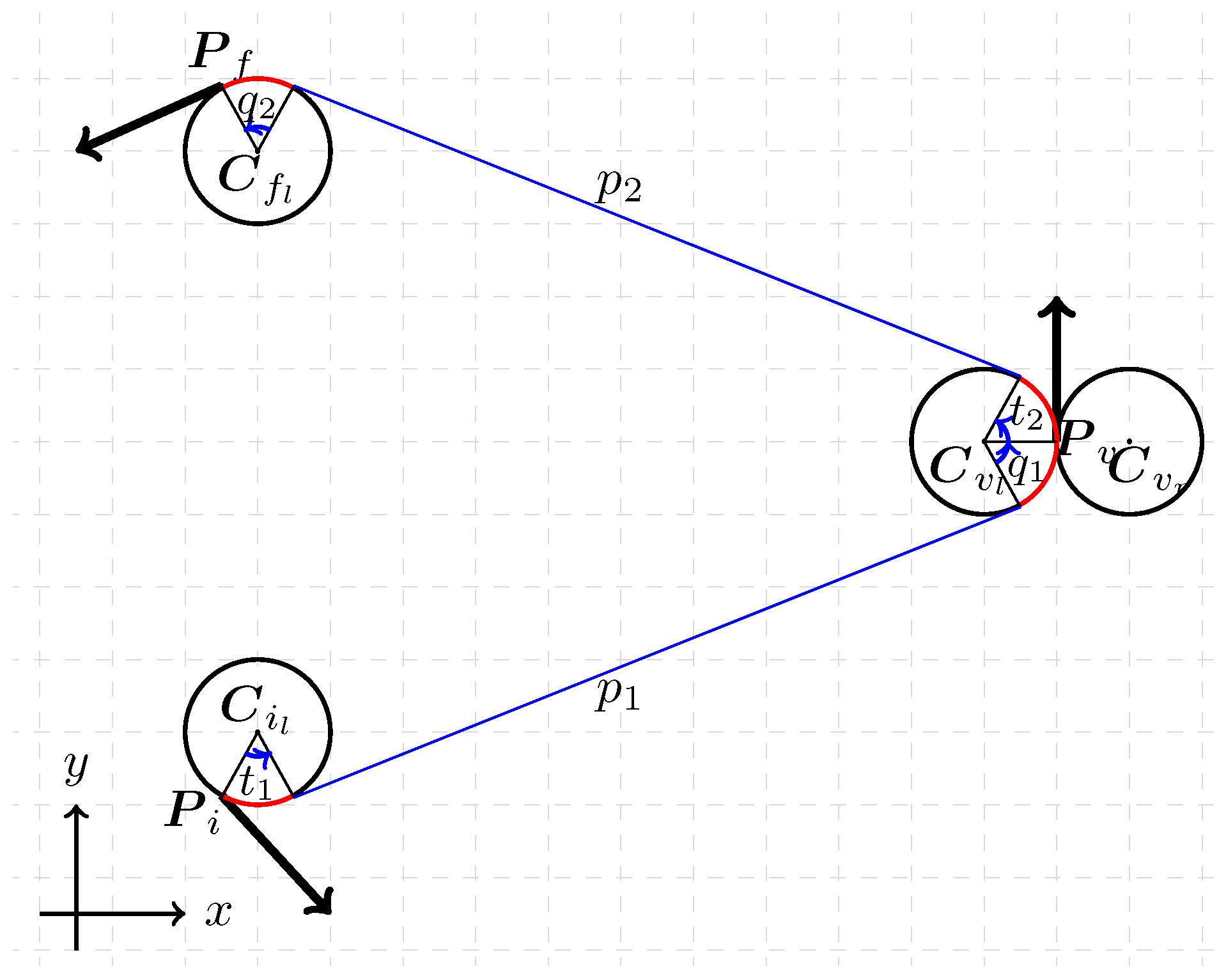
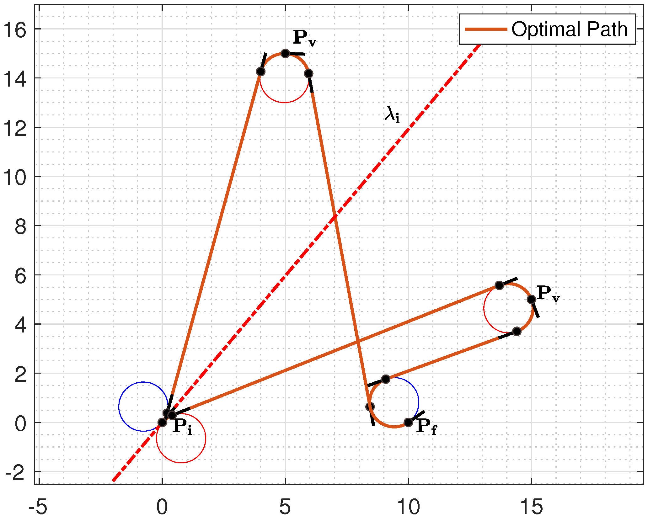
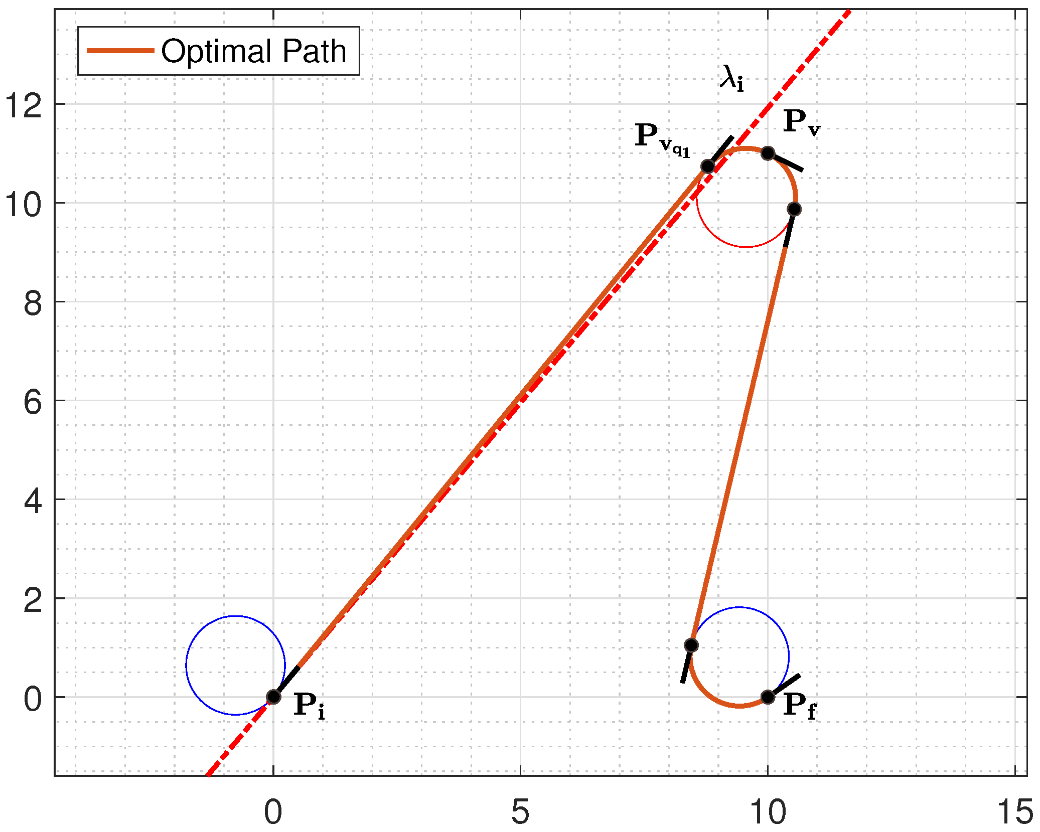
4. An Illustrative Example

In this section, we provide a simple example to illustrate how the proposed classification rules work, demonstrating the functionality of the proposed algorithms. Let us consider the following initial and final configurations: ${\mathbf{q}}_i(0,0,50°)$, ${\mathbf{q}}_f(10,0,35°)$, a maximal curvature $\mathrm{\Omega }=1$, and the via point $P_v=(-10,15)$ (see Figure 19).

The optimal path type has the form “$C_{initial}S{C}_{viaPoint}-C_{viaPoint}S{C}_{final}$”; thus, we need to identify the curvature at the initial point, at the final point, and at the via point. We can rely on the heuristic approach—more practical with respect to the analytical counterpart. Applying Algorithm 2 since ${\theta }_i\in Q_I$ and ${\mathit{P}}_v\in {\pi }_{{\lambda }_i}^l$, we immediately deduce that $C_{initial}=L$. Similarly, by applying Algorithm 4 since ${\theta }_i\in Q_I$ and ${\mathit{P}}_v\in {\pi }_{{\lambda }_f^l}^l$, we immediately deduce that $C_{final}=L$. With reference to the curvature at the via point, since the initial and final configurations are both in the first quadrant, and the via point is on Region 2, we can apply Algorithm 8. This allows us to deduce that $C_{viaPoint}=R$. Thus, we can directly deduce the optimal path type without making any calculations.

Following a conventional approach, the optimal solution would be found by searching among the eight candidate paths: $\{RSR-RSR,LSR-RSR,RSR-RSL,LSR-RSL,LSL-LSL,RSL-LSL,LSL-LSR,RSL-LSR\}$ using any of the existing methods in the literature, such as those presented in references [17,18,29]. By applying one of these methods, the lengths of the eight candidate paths would be calculated and compared to determine the optimal path.

5. Numerical Results

In this section, we evaluate the performance of the proposed method. We conducted an experiment on random tuples (${\mathbf{q}}_i$, ${\mathit{P}}_v$, ${\mathbf{q}}_f$). The points ${\mathit{P}}_i$, ${\mathit{P}}_v$, and ${\mathit{P}}_f$ were randomly selected in a $10\times 10$ environment with the minimum distance between any pair of points equal to $4{\mathrm{\Omega }}^{-1}$, being $\mathrm{\Omega }=1$. For each tuple, we applied the shortest path synthesis to identify the (potentially) optimal path types. Then, we solved only the three-point Dubins path problem for the specific path type identified. This can be performed by resorting to any of the methods in the literature, such as [17,18,29]. Here, the approach based on analytic geometry tools proposed in [29] was considered. For the sake of clarity of exposition, we denote it as the Geometry-Based Method (GBM) hereafter. The results of this numerical experiment are evaluated in terms of execution time.

Here, $T_{GBM}$ represents the execution time for solving the 3PDP using the GBM, while $T_{CL}$ refers to the execution time when applying the GBM exclusively to the optimal path types identified by the proposed classification rules. We can define the average factor of improvement I over M runs for a given method with respect to the GBM as follows:

$$\begin{array}{c}\hfill I={\displaystyle \frac{1}{M}}\sum _{j=1}^M{\displaystyle \frac{T_{GBM}\left(j\right)}{T_{CL}\left(j\right)}}\end{array}$$

(28)

The simulation results confirm the benefits of including the shortest path synthesis into the three-point Dubins path planning. Indeed, as shown in Table 1, it reduced the required computational cost by half, resulting in a doubled improvement factor compared to a method that is already characterized for its fast computational time, as highlighted in [29]. Thus, the proposed classification rules speed up the planning algorithm, making it much more efficient with respect to the counterpart that does not use the classification.

Table 1. The average factor of improvement in runtime on M = 30 instances with the use of the proposed classification rules over the Geometry-Based method.

	Improvement (I)
Classification	$1.96$

From a computational point of view, Table 1 provides the average factor of improvement in runtime on M = 30 instances using the GBM with the use of the proposed classification rules. The algorithms were coded in MATLAB^® (version R2020b) on an Apple Laptop with a 3.1 GHz Intel Core i7 processor, 16 GB RAM, running a MAC OS X Version 10.15.7 operating system. Also, note that the MATLAB implementations of the planning algorithms were not specifically optimized for execution time. Of course, by using dedicated hardware and a suitably optimized code, the execution time can be significantly less. So, the proposed classification strategy can be readily exploited in real-time applications because of its ability to reduce the computational effort of three-point Dubins path planning algorithms.

6. Conclusions

In this paper, we present a shortest path-type classification between an initial and a final configuration passing through an intermediate via point for a Dubins vehicle. The proposed methodology allows us to select the optimal path type without any calculations; hence, it is suitable to be used in real-time applications. The proposed strategy is described through the explanation of a simple worked example. Future research will include the extension of the approach to a time-varying and multi-robot scenario, as well as the use of the algorithm in practice.

References

- Lin, S.; Liu, A.; Wang, J.; Kong, X. A Review of Path-Planning Approaches for Multiple Mobile Robots. Machines 2022, 10, 773. [Google Scholar] [CrossRef]
- Tang, Y.; Qi, S.; Zhu, L.; Zhuo, X.; Zhang, Y.; Meng, F. Obstacle avoidance motion in mobile robotics. J. Syst. Simul. 2024, 36, 1. [Google Scholar]
- Molina, B.; Palau, C.E.; Calvo-Gallego, J. Unified Travel Solutions: Bridging Outdoor Route Planning with Intelligent Indoor Navigation. J. Data Sci. Intell. Syst. 2024. [Google Scholar] [CrossRef]
- LaValle, S.M. Planning Algorithms; Cambridge University Press: Cambridge, MA, USA, 2006. [Google Scholar]
- Dubins, L.E. On curves of minimal length with a constraint on average curvature, and with prescribed initial and terminal positions and tangents. Am. J. Math. 1957, 79, 497–516. [Google Scholar] [CrossRef]
- Boissonnat, J.D.; Cérézo, A.; Leblond, J. Shortest paths of bounded curvature in the plane. J. Intell. Robot. Syst. 1994, 11, 5–20. [Google Scholar] [CrossRef]
- Bicchi, A.; Pallottino, L. On Optimal Cooperative Conflict Resolution for Air Traffic Management Systems. IEEE Trans. Intell. Transp. Syst. 2000, 1, 221–231. [Google Scholar] [CrossRef]
- Savla, K.; Frazzoli, E.; Bullo, F. Traveling salesperson problems for the Dubins vehicle. IEEE Trans. Autom. Control 2008, 53, 1378–1391. [Google Scholar] [CrossRef]
- Meyer, Y.; Isaiah, P.; Shima, T. On Dubins paths to intercept a moving target. Automatica 2015, 53, 256–263. [Google Scholar] [CrossRef]
- Shkel, A.M.; Lumelsky, V. Classification of the Dubins set. Robot. Auton. Syst. 2001, 34, 179–202. [Google Scholar] [CrossRef]
- Consonni, C.; Brugnara, M.; Bevilacqua, P.; Tagliaferri, A.; Frego, M. A new Markov–Dubins hybrid solver with learned decision trees. Eng. Appl. Artif. Intell. 2023, 122, 106166. [Google Scholar] [CrossRef]
- Xue, P.; Pi, D.; Wan, C.; Yang, C.; Xie, B.; Wang, H.; Wang, X.; Yin, G. Collaborative planning and control of heterogeneous multi-ground unmanned platforms. Eng. Appl. Artif. Intell. 2024, 136, 108968. [Google Scholar] [CrossRef]
- Berdyshev, Y. Time-optimal control of a nonlinear system in the problem of visiting a group of points. Cybern. Syst. Anal. 1991, 27, 949–952. [Google Scholar] [CrossRef]
- Berdyshev, Y. A problem of the sequential approach to a group of moving points by a third-order non-linear control system. J. Appl. Math. Mech. 2002, 66, 709–718. [Google Scholar] [CrossRef]
- Kaya, C. Markov-Dubins interpolating curves. Comput. Optim. Appl. 2019, 73, 647–677. [Google Scholar] [CrossRef]
- Frego, M.; Bevilacqua, P.; Saccon, E.; Palopoli, L.; Fontanelli, D. An iterative dynamic programming approach to the multipoint markov-dubins problem. IEEE Robot. Autom. Lett. 2020, 5, 2483–2490. [Google Scholar] [CrossRef]
- Sadeghi, A.; Smith, S.L. On efficient computation of shortest dubins paths through three consecutive points. In Proceedings of the 2016 IEEE 55th Conference on Decision and Control (CDC), Las Vegas, NV, USA, 12–14 December 2016; pp. 6010–6015. [Google Scholar]
- Chen, Z.; Shima, T. Shortest Dubins paths through three points. Automatica 2019, 105, 368–375. [Google Scholar] [CrossRef]
- Parlangeli, G.; Ostuni, L.; Mancarella, L.; Indiveri, G. A motion planning algorithm for smooth paths of bounded curvature and curvature derivative. In Proceedings of the Mediterranean Conference on Control and Automation(MED), Thessaloniki, Greece, 24–26 June 2009; pp. 73–78. [Google Scholar]
- Parlangeli, G.; Indiveri, G. Dubins inspired 2D smooth paths with bounded curvature and curvature derivative. IFAC Proc. Vol. 2010, 43, 252–257. [Google Scholar] [CrossRef]
- Hota, S.; Ghose, D. Optimal trajectory planning for unmanned aerial vehicles in three-dimensional space. J. Aircr. 2014, 51, 681–688. [Google Scholar] [CrossRef]
- Becce, L.; Bloise, N.; Guglieri, G. Optimal path planning for autonomous spraying uas framework in precision agriculture. In Proceedings of the 2021 International Conference on Unmanned Aircraft Systems (ICUAS), Athens, Greece, 15–18 June 2021; pp. 698–707. [Google Scholar]
- Hansen, K.D.; La Cour-Harbo, A. Waypoint planning with Dubins curves using genetic algorithms. In Proceedings of the 2016 European Control Conference (ECC), Aalborg, Denmark, 29 June–1 July 2016; pp. 2240–2246. [Google Scholar]
- Zhu, M.; Zhang, X.; Luo, H.; Wang, G.; Zhang, B. Optimization Dubins path of multiple UAVs for post-earthquake rapid-assessment. Appl. Sci. 2020, 10, 1388. [Google Scholar] [CrossRef]
- Du, X.; Li, X.; Liu, D.; Dai, B. Path planning for autonomous vehicles in complicated environments. In Proceedings of the 2016 IEEE International Conference on Vehicular Electronics and Safety (ICVES), Beijing, China, 10–12 July 2016; pp. 1–7. [Google Scholar]
- Bayar, G. Reference path generation and obstacle avoidance for autonomous vehicles based on waypoints, dubins curves and virtual force field method. Int. J. Appl. Math. Electron. Comput. 2017, 5, 1–6. [Google Scholar] [CrossRef]
- Sharma, K.; Doriya, R. Coordination of multi-robot path planning for warehouse application using smart approach for identifying destinations. Intell. Serv. Robot. 2021, 14, 313–325. [Google Scholar] [CrossRef]
- Cai, W.; Zhang, M.; Zheng, Y.R. Task assignment and path planning for multiple autonomous underwater vehicles using 3D dubins curves. Sensors 2017, 17, 1607. [Google Scholar] [CrossRef] [PubMed]
- Parlangeli, G.; De Palma, D.; Attanasi, R. A novel approach for 3PDP and real-time via point path planning of Dubins’ vehicles in marine applications. Control Eng. Pract. 2024, 144, 105814. [Google Scholar] [CrossRef]
- Goaoc, X.; Kim, H.S.; Lazard, S. Bounded-curvature shortest paths through a sequence of points using convex optimization. SIAM J. Comput. Soc. Ind. Appl. Math. 2013, 42, 662–684. [Google Scholar] [CrossRef]
Disclaimer/Publisher’s Note: The statements, opinions and data contained in all publications are solely those of the individual author(s) and contributor(s) and not of MDPI and/or the editor(s). MDPI and/or the editor(s) disclaim responsibility for any injury to people or property resulting from any ideas, methods, instructions or products referred to in the content. |
© 2024 by the authors. Licensee MDPI, Basel, Switzerland. This article is an open access article distributed under the terms and conditions of the Creative Commons Attribution (CC BY) license (https://creativecommons.org/licenses/by/4.0/).