Fault Diagnosis Method for Tractor Transmission System Based on Improved Convolutional Neural Network–Bidirectional Long Short-Term Memory

Abstract

In response to the problems of limited algorithms and low diagnostic accuracy for fault diagnosis in large tractor transmission systems, as well as the high noise levels in tractor working environments, a defect detection approach for tractor transmission systems is proposed using an enhanced convolutional neural network (CNN) and a bidirectional long short-term memory neural network (BILSTM). This approach uses a one-dimensional convolutional neural network (1DCNN) to create three feature extractors of varying scales, directly extracting feature information from different levels of the raw vibration signals. Simultaneously, in order to enhance the model’s predicted accuracy and learn the data features more effectively, it presents the multi-head attention mechanism (MHA). To overcome the issue of high noise levels in tractor working environments and enhance the model’s robustness, an adaptive soft threshold is introduced. Finally, to recognize and classify faults, the fused feature data are fed into a classifier made up of bidirectional long short-term memory (BILSTM) and fully linked layers. The analytical findings demonstrate that the fault recognition accuracy of the method described in this article is over 98%, and it also has better performance in noisy environments.

1. Introduction

As a crucial component of agricultural mechanization, tractors play a significant role in agricultural production. Equipped with various implements, tractors can efficiently perform tasks such as land cultivation and planting, thereby reducing the labor intensity of farmers and enhancing agricultural productivity [1]. However, tractors face numerous challenges [2], including the need to transmit large amounts of power, a wide range of speed variations, harsh operating environments, and frequent load fluctuations. Once the tractor’s transmission system experiences a decrease in reliability or even serious failure, it not only delays agricultural operations and affects crop yields but also compromises the overall safety of the tractor [3,4]. As a result, diagnosing issues with large tractors’ transmission systems is crucial.

With the advancement of agricultural mechanization, tractors are evolving towards larger and more intelligent configurations. The complexity of tractor transmission systems has increased with this development, leading to a diverse range of potential faults [5]. As a result, traditional fault diagnosis methods are no longer adequate. During operation, components like the gearbox of tractors generate vibrations. A commonly used deep learning fault diagnosis method involves analyzing information from these vibration signals to detect issues with the gearbox [6,7]. Gangsar, Purushottam et al. [8]. employed deep learning techniques for state detection and fault diagnosis of rotating. Feng et al. [9] proposed an adaptive spiral flight SSA algorithm to eliminate the interference components caused by noise and vibration sources. This method is a Gaussian Laplacian (LoG) filtering technique optimized by improving the sparrow search algorithm (SSA), and its effectiveness has been verified through experiments. Wang et al. [10] proposed a lightweight fault diagnosis method based on an attention mechanism and multi-layer fusion network, which addresses the conflict between the large number of parameter calculations in deep networks and the current embedded platform computing resources. This method proposes a lightweight student network that reduces computational complexity and improves computing speed while ensuring accuracy. Saadi et al. [11] proposed a novel BILSTM neural network that extracts frequency characteristics from two-dimensional images of vibration signals and recombines frequency data from vibration images to improve fault recognition accuracy. Guo et al. [12] proposed a method based on attention CNN and BILSTM (ACNN-BILSTM) to solve the problem of existing bearing fault diagnosis methods being unable to adaptively select features and difficult to handle noise interference. This method introduces a convolutional block attention module that reallocates weights between different feature dimensions, improving the model’s attention to important features and achieving a high fault recognition rate.

Intelligent algorithms have been widely used in a variety of pattern recognition domains, including image processing [13], computer vision [14], natural language processing [15], and medicine [16], thanks to the development of deep learning technology. Concurrently, related algorithms are also increasingly utilized in mechanical fault diagnosis. Algorithms for defect diagnosis have been becoming more sophisticated and intelligent in recent years. For bearing defect identification, Zhang et al. [17] proposed a multi-scale deep residual shrinkage network with a mixed attention mechanism to address the impact of unexpected noise caused by accessible vibration signals and global information attenuation in deep networks during fault diagnosis. This method introduces a spatial domain attention mechanism in the residual shrinkage module and constructs a mixed attention mechanism that takes into account both internal and cross channel characteristics. The combination of DRSN and dilated convolution features enhances the global fault information of rolling bearings and improves the accuracy of the model under noise interference. A novel signal decomposition method called empirical standard autoregressive power spectral decomposition was presented by Zhang et al. [18]. This method can effectively decompose bearing fault signals and identify all fault characteristics. With an accuracy of 94.08%, Ravikumar, K.N. et al. [19] presented a fault diagnostic model that combines residual learning [20] and convolutional neural networks (CNNs) [21] for bearing and gear problem identification. A novel approach to defect diagnostics for tractor gearboxes was put out by Mohammad Hosseinpour-Zarnaq et al. [22]. With a 95% accuracy rate, this approach uses vibration signals from gears and Random Forest (RF) [23] and Multi-Layer Perceptron (MLP) [24] neural networks for data classification. Most of the methods described above involve processing the original vibration signals using algorithms such as Continuous Wavelet Transform (CWT), Discrete Wavelet Transform (DWT), Fast Fourier Transform (FFT) [25,26], etc. Then, the synchrosqueezed transform (SST) [27] is used to compress the signal and improve the resolution. Finally, the data are converted into two-dimensional images combined with neural networks for fault recognition and classification. Although synchrosqueezed transform (SST) technology can improve the quality of signal analysis, it requires high computational costs and processing power. In addition, during the process of converting one-dimensional signals, crucial information along the time series may be lost [28], ultimately affecting the accuracy of recognition. Additionally, converting one-dimensional signals into images can increase computational complexity and storage requirements [29]. Huang et al. [30] conducted an analysis of the feature extraction mechanism of one-dimensional convolutional neural networks, revealing that they exhibit excellent learning capabilities for time series data. Sun et al. [31] used one-dimensional convolutional neural networks to diagnose bearing faults, and the results were highly accurate. The aforementioned methods yield satisfactory results in traditional fault diagnosis scenarios such as gearboxes and bearings. However, extensive data preprocessing is required before classification, leading to complex network structures, indicating room for optimization in terms of the structure and efficiency of these algorithms for fault diagnosis. Additionally, these algorithms do not address the issue of noise interference in the harsh working environments of tractors, rendering them potentially unsuitable for fault diagnosis in modern tractor transmission systems.

The general procedure of fault diagnosis involves data collection, data preparation, feature extraction, identification, and classification. An essential component of fault detection is feature extraction [32]. Thus, using bidirectional long short-term memory (BILSTM) and one-dimensional convolutional neural networks (1DCNNs), this research suggests a defect detection technique for tractor transmission systems. The method aims to enhance fault recognition accuracy and robustness by improving the CNN network to construct a novel feature extractor. Firstly, different scales of feature extractors are constructed using one-dimensional convolutional neural networks (1DCNNs) to directly extract feature information at different levels. Secondly, in order to enhance feature learning and increase the accuracy of defect recognition, a multi-head attention mechanism (MHA) is introduced. Additionally, an adaptive soft threshold is incorporated to further improve the model’s resilience and capacity for generalization. Finally, to accomplish fault recognition and classification, the fused features are fed into a classifier made up of completely linked layers and bidirectional long short-term memory (BILSTM).

2. Theoretical Foundation

2.1. 1DCNN

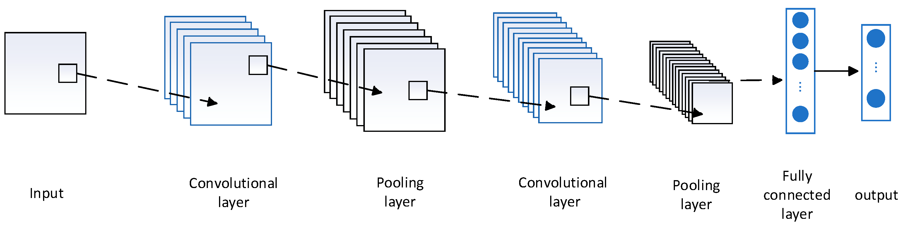
One kind of deep learning model made especially for handling data with grid-like structures is the convolutional neural network (CNN). In domains including natural language processing, computer vision, and image recognition, CNNs have had great success. CNNs are mainly utilized as feature extractors in the defect diagnostic domain, which involves taking raw data input and extracting higher-level information for use in the following tasks. Convolutional layers, activation functions, pooling layers, and fully linked layers make up CNNs in their whole. As illustrated in Figure 1, CNNs gradually extract abstract features from the input data by stacking these components layer by layer, and weights are adjusted during training to reduce the discrepancy between expected and actual values.

Figure 1. Convolutional neural network structure diagram.

One-dimensional convolutional neural networks (1DCNNs) are primarily employed in handling time-series data, audio signals, natural language processing, and other related domains. Structurally, they do not differ from traditional convolutional neural networks.

(1)

Convolutional layer

A convolutional layer is a kind of core neural network layer, which is very important in the network structure. Through convolutional operation and specific design principles, the model can effectively extract features and reduce the number of parameters to enhance the model’s understanding of data and generalization ability. The convolutional layer computes using the following method:

$$\mathrm{A}{y}_i^l=f_{act}\left(k_i^{l-1}\sum x_i^{l-1}+b_i^l\right)$$

(1)

where $f_{act}$ represents the activation function; the convolutional kernel, or weights, connected to the i-th neuron in the $l-1$ layer is represented by $k_i^{l-1}$; the bias term of the i-th neuron in the $l$-th layer is represented by $b_i^{l-1}$; $x_i^{l-1}$ represents the output of the neuron connected to the i-th convolutional kernel in the $l-1$ layer; and $y_i^l$ represents the output of the i-th neuron in the $l$-th layer.

(2)

Activation function

The activation function mainly plays a role in introducing nonlinearity, solving the problem of vanishing gradients and increasing the expression ability of the network. Selecting the appropriate activation function can improve the computational efficiency of the network. As demonstrated below, the tanh function is the activation function that is used in this paper.

$$\mathit{tanh}\left(x\right)={\displaystyle \frac{2}{1+e^{-2x}}}-1$$

(2)

(3)

Pooling layer

The pooling layer is mainly used to reduce the dimensions and parameters of the data to reduce computation and control overfitting. Mean-pooling and max-pooling are two popular pooling operations. The max-pooling method, which chooses the maximum value inside a region, is used in this research to minimize parameters.

$$P_i^l\left(j\right)=\underset{\left(j-1\right)W+1\le t\le jW}{max}\left\{x_i^l\right\}$$

(3)

where${ x}_i^l$ is the pooled value, and $W$ denotes the pooling kernel’s size. $\left(j-1\right)W+1\le t\le jW$represents the index range of the pooling window, and $P_i^l\left(j\right)$ represents the output of the i-th pooling window in the $l$-th layer.

(4)

Fully connected layer

In order to integrate and categorize the information retrieved by the convolutional and pooling layers, each node in the fully connected layer is connected to every other node in the previous layer, creating a completely connected network structure. And then the loss function is calculated to evaluate the model. The fully connected layer is generally used at the end of the network as the output layer.

2.2. Multi-Head Attention Mechanism

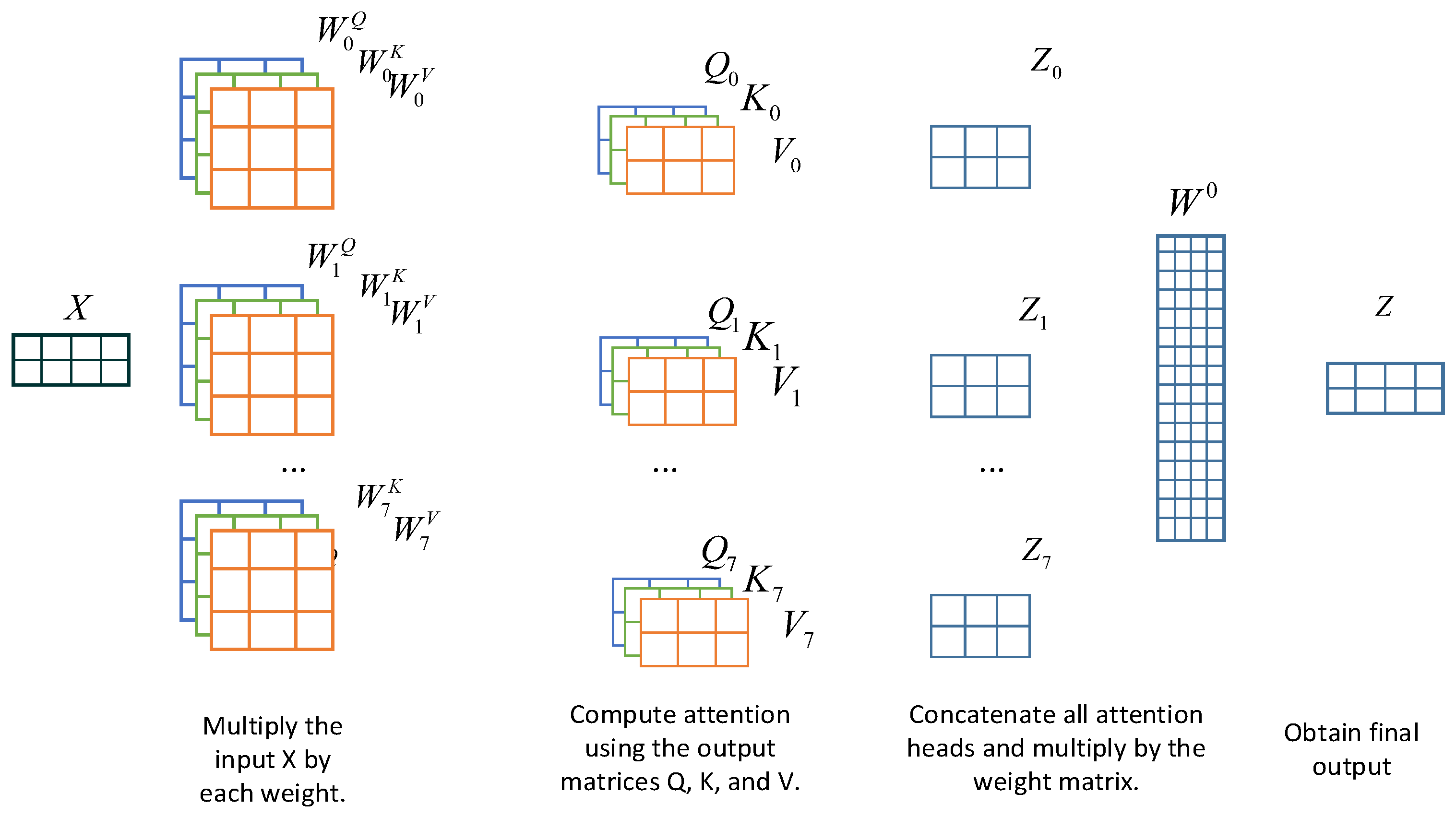
It is possible to think of the attention process as a resource allocation system, which can increase the weight of effective features during the feature extraction process, thus improving the efficiency of feature extraction under limited computational resources [33]. The attention mechanism is expanded upon in multi-head attention, introducing multiple sets of queries, keys, and values, each set referred to as a “head”. These heads run in parallel, independently computing attention weights and outputs, and the resulting outputs are concatenated and linearly transformed to obtain the final output. The structure of multi head attention is shown in Figure 2.

Figure 2. Multi-head attention structure diagram.

Using multi-head attention, the model may learn distinct characteristics in several subspaces, thus better capturing the complex relationships and representations of input sequences. One-dimensional convolutional neural networks primarily focus on extracting local features, but by introducing multi-head attention, the network can simultaneously attend to information and features at different positions in the sequence and conduct correlated learning in multiple subspaces. This improves the model’s capacity to extract information and generalize it to other tasks.

2.3. Adaptive Soft Thresholding

Because of how noise and other environmental elements affect actual work environments, inspired by the deep residual shrinkage network (DRSN) [34], an adaptive soft thresholding module is introduced to mitigate the impact of noise on data while also improving the model’s robustness. Soft thresholding is a nonlinear function that sets signal values below a threshold to zero while preserving those above it to achieve denoising. Soft thresholding is generally expressed as follows:

$$S_{\lambda }\left(x\right)=sign\left(x\right)\cdot \left(\left|x\right|-\lambda \right)+$$

(4)

where $S_{\lambda }\left(x\right)$ is the output signal; and $\mathrm{sign}\left(x\right)$ is the sign function, which returns 1 when x > 0, −1 when x < 0, and 0 when x = 0. This function is used to maintain the sign of x; and ()+ denotes taking the positive part. $\left|x\right|$represents the absolute value of the input value, and λ is a threshold parameter that determines the degree of contraction. The adaptive soft thresholding introduces a learnable parameter, which is trained alongside other parameters of the neural network and updated through gradient descent. This enables the network to achieve denoising effects by dynamically learning and adjusting the threshold based on the properties of the data.

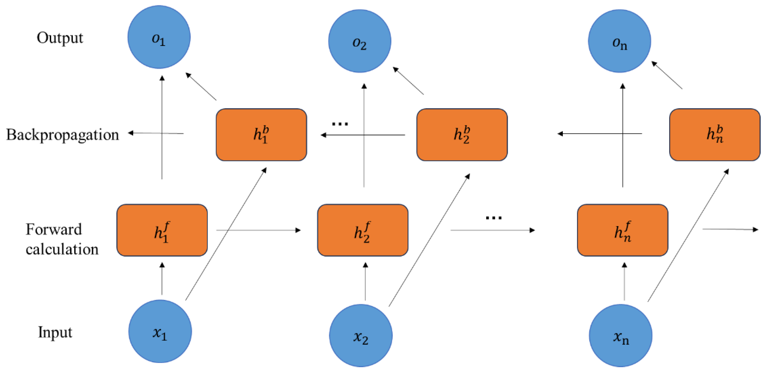
2.4. BILSTM Network

Long short-term memory (LSTM) is a variant proposed to address issues like the gradient vanishing problem in recurrent neural networks (RNNs). It features memory units that can better capture information and relationships in sequential data [35]. Moreover, gate components including input, forget, and output gates are used by LSTM to regulate information flow and update memory. Consequently, it offers benefits when managing time-series data.

The bidirectional long short-term memory (BILSTM) network extends the traditional LSTM by incorporating an additional layer for backward computation. The results from both directions are concatenated to give a more thorough understanding of the data. The structure of BILSTM is shown in Figure 3:

Figure 3. BILSTM structure diagram.

The computation formula for BILSTM is as follows:

$$h_t^f=f^f\left(w_1{x}_t+w_2{h}_{t-1}\right)$$

(5)

$${ h}_t^b=f^b\left(w_3{x}_t+w_4{h}_{t-1}\right)$$

(6)

$$o_t=f\left(w_5{h}_t^f+w_6{h}_t^b\right)$$

(7)

where the result of the forward computation is denoted by $h_t^f$, and the activation function of forward calculation is denoted by $f^f$. $w_1$ and $w_2$ are weight coefficients that connect the input $x_t$ of the current time step and the output $h_{t-1}$ of the previous time step with the internal state of LSTM; $h_t^b$ represents the result of conducting a reverse calculation; $f^b$ is the activation function for reverse calculation; $w_3$ and $w_4$ represent weights, which have the same effect as the weights calculated in the forward direction; the network’s ultimate output is denoted by $o_t$; $f$ is the activation function of the output layer; and $w_5$ and $w_6$ represent weights, connecting the forward calculated output with the backward calculated output.

3. Improved Feature Extraction Network

3.1. Subsection

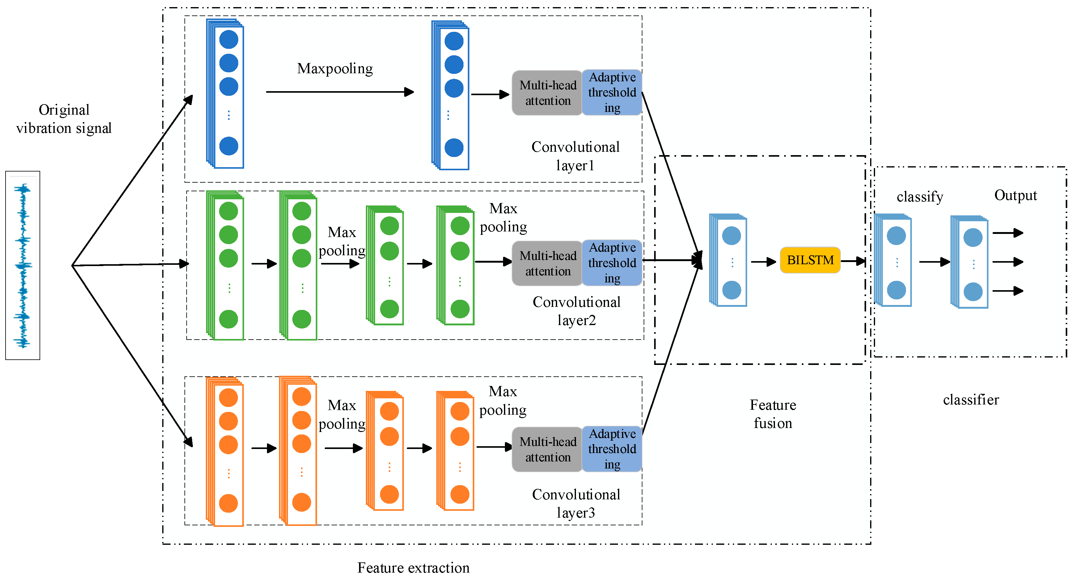
The model presented in this paper is mainly composed of a new feature extractor, a feature fusion module, and a softmax classifier. These are created by integrating an adaptive soft thresholding module, enhanced CNN-LSTM network, and a multi-head attention mechanism (MHA), as shown in Figure 4.

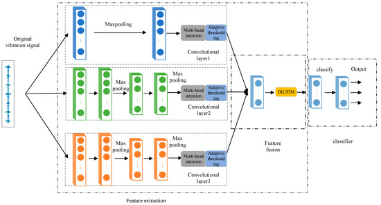
Figure 4. Network structure diagram.

3.2. Method for Diagnosing Faults Using the Proposed Feature Extraction Network

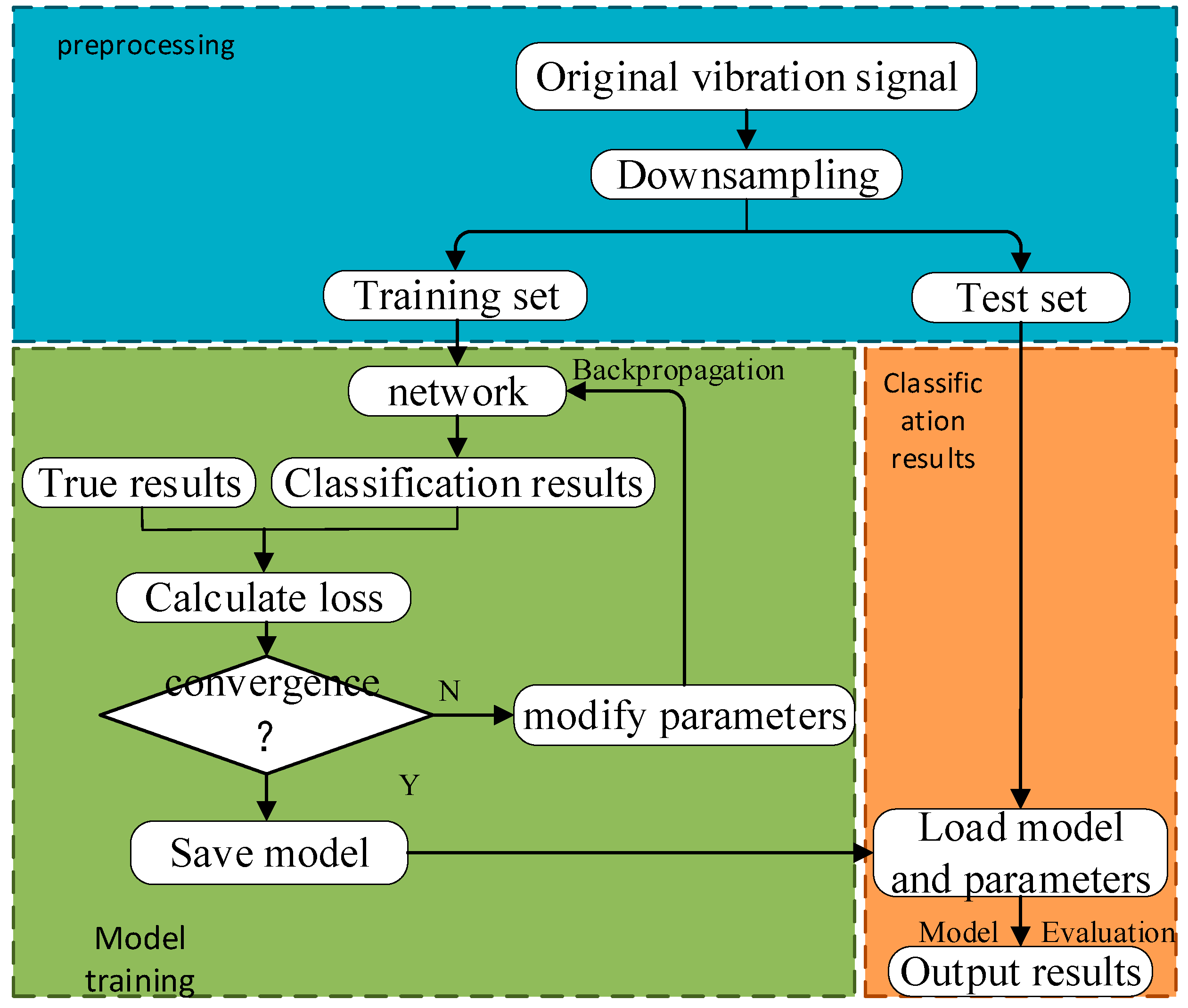
The proposed fault diagnosis process for tractor transmission systems based on improved 1DCNN-BILSTM is illustrated in Figure 5. The steps that are specific are as follows: Firstly, a proportionate downsampling and division of the original vibration signals is made into training and testing sets. After the training data have been normalized and put into the network, the model is stored and the loss is determined using mean squared error. Then, the trained model uses the testing set to determine the accuracy, recall rate, and F1 score for model assessment. Finally, the model is applied to fault diagnosis in the tractor transmission system.

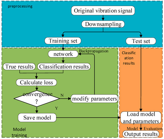
Figure 5. Fault diagnosis flowchart.

4. Experimental Verification and Analysis

4.1. Dataset Description

4.1.1. CWRU Bearing Database

Experiments were carried out utilizing the rolling bearing dataset from Case Western Reserve University (CWRU) [36] and the gearbox dataset gathered in the lab to verify the efficacy of the model.

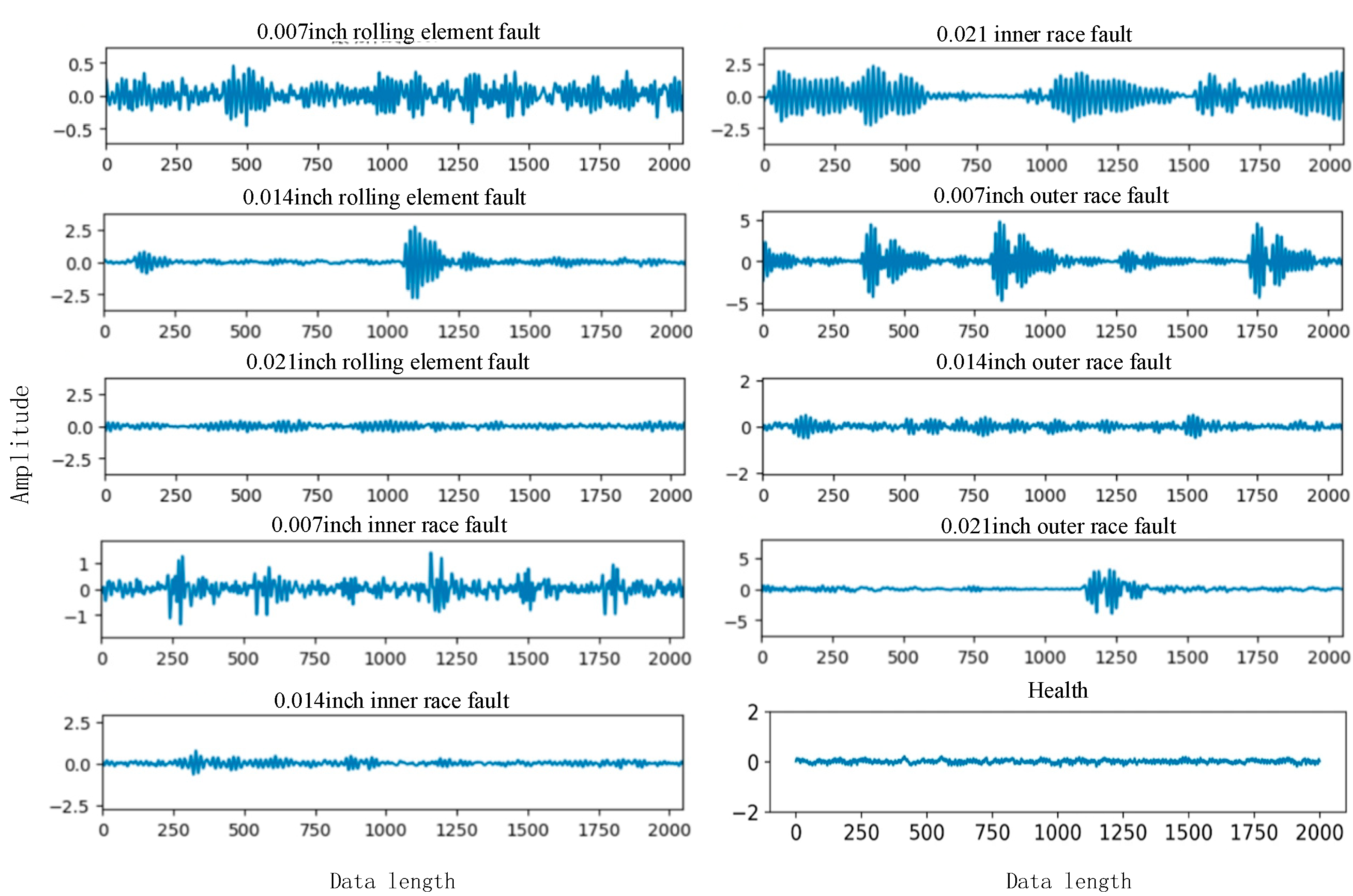
Vibration signals from the motor’s drive end (DE), with a sample frequency of 48 kHz, a motor speed of 1750 rpm, and power of 3 HP, are used in the CWRU bearing database. Bearings are categorized into three distinct fault types and a healthy state, namely, outer race fault, rolling element fault, and inner race fault. Three distinct fault diameters are configured for each type of fault, resulting in a total of ten datasets, and 240 observations are taken for each type of data, with each sample length of 2000. The training sets and testing sets consist of a collection of 2400 data points, divided in a 7:3 ratio. The Table 1 lists the different kinds of signal samples along with the labels that go with them.

Table 1. Dataset.

Label	Fault	Fault Size	Number of Observations
0	rolling element fault	0.007	240
1	rolling element fault	0.014	240
2	rolling element fault	0.021	240
3	inner race fault	0.007	240
4	inner race fault	0.014	240
5	inner race fault	0.021	240
6	outer race fault	0.007	240
7	outer race fault	0.014	240
8	outer race fault	0.021	240
9	normal	—	240

Figure 6 shows the waveforms of the original vibration signals related to different types of faults. It can be seen from the figure that each fault type corresponds to a vibration image, and the method proposed in this paper can extract and learn the unique characteristic information of each fault for identification and classification.

Figure 6. Original vibration signal plot.

4.1.2. Collected Gear Dataset

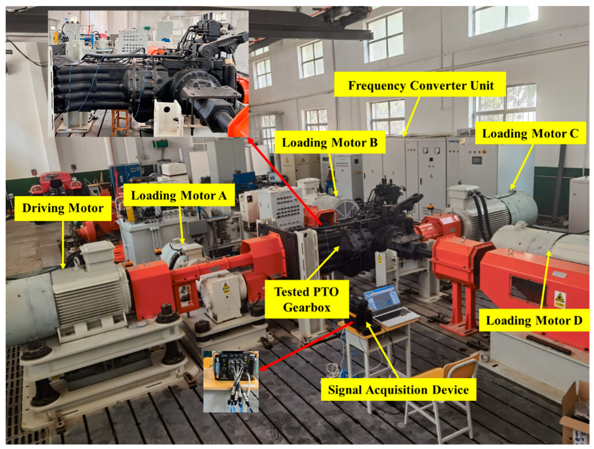
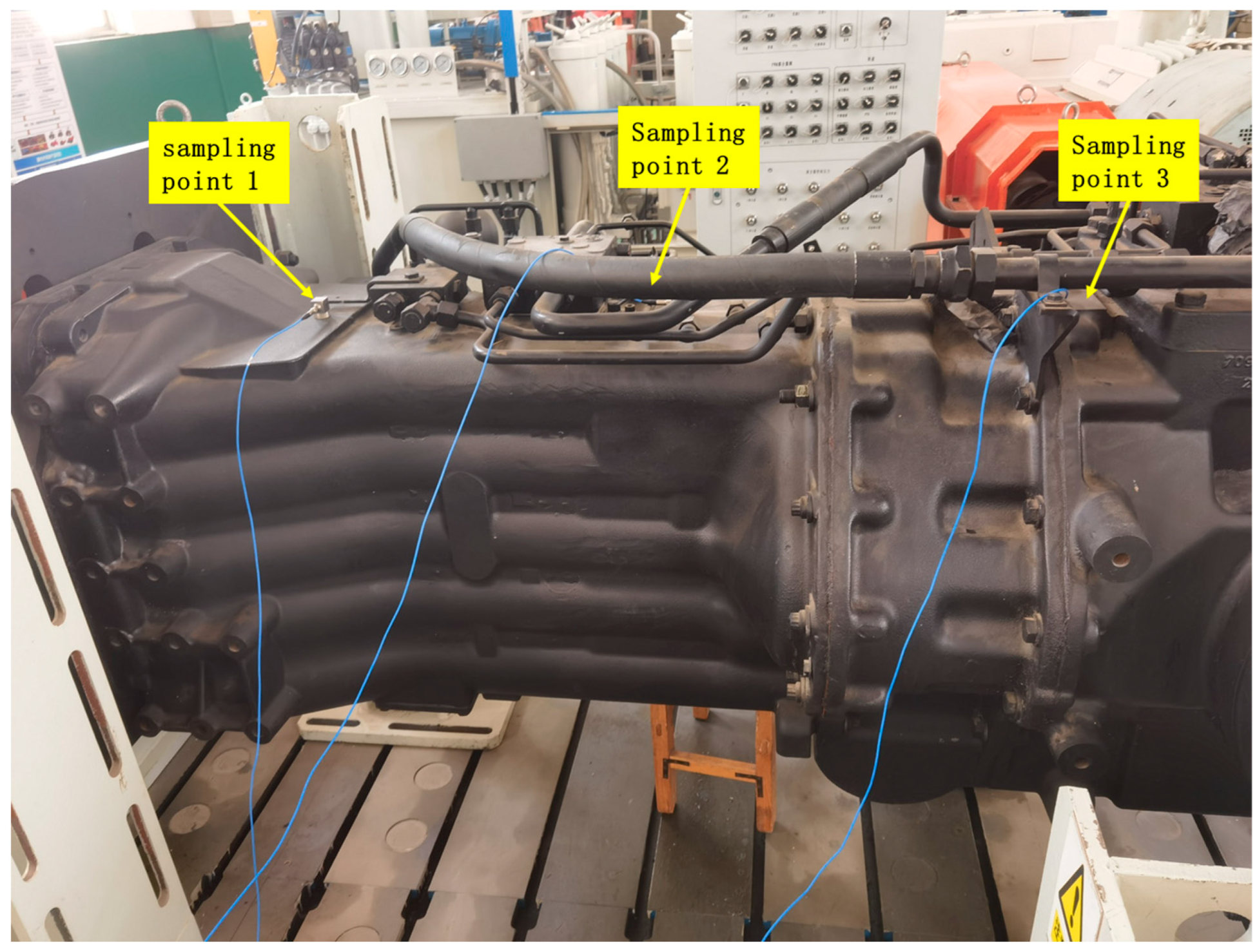
The laboratory utilized a tractor transmission system test bench to collect vibration data from the gearbox by using the DH5902 data acquisition and analysis system, with acceleration sensors mounted on the gearbox to capture vibration signals. The sampling frequency was 48 KHz and recorded the collected temporal data in CSV format. Because in practical application scenarios, tractors mainly operate under relatively stable working conditions, this experiment only considers faults under constant speed conditions. Figure 7 depicts the physical layout of the test bench, and Figure 8 shows the installation position of the accelerometer; we set a total of three sampling points on the gearbox, and ultimately used the vibration data of the planetary gears at sampling point 2.

Figure 7. Tractor transmission system loading test bench.

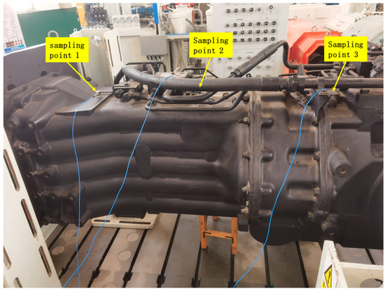
Figure 8. Schematic diagram of sampling point location.

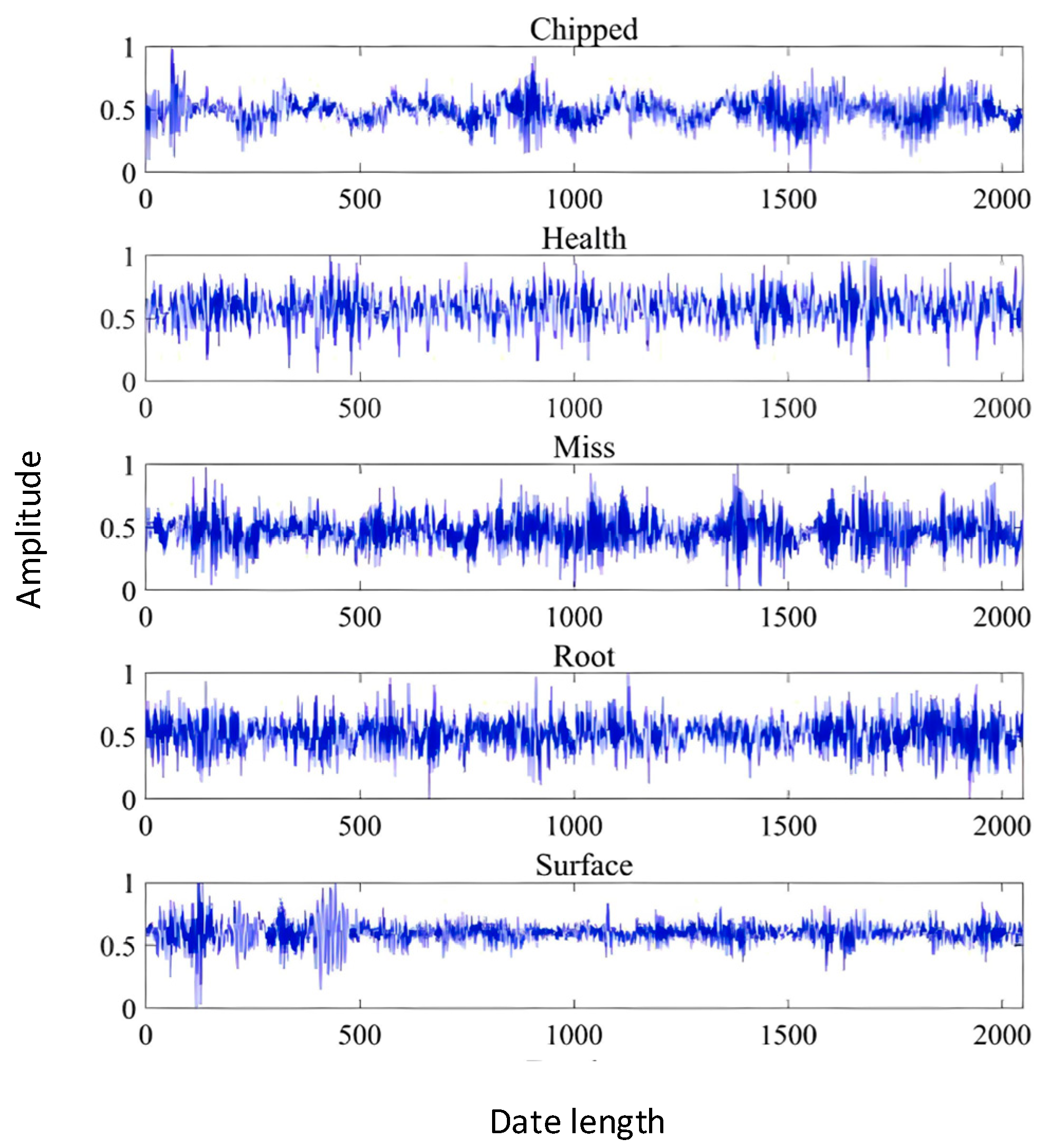
The tractor transmission system loading test bench mainly consists of the driving unit, front drive loading unit, left rear axle loading unit, right rear axle loading unit, PTO loading unit, PTO gearbox, and frequency converter assembly unit. This test platform simulates the operating conditions of the gearbox in a tractor transmission system. As shown in Figure 8, the accelerometer is installed on the PTO transmission to collect gear data during transmission operation. The loading test bench is used to simulate the actual working conditions of the tractor in the field. The gear fault states are divided into five categories: normal, root crack, broken tooth, missing tooth, and tooth surface wear; 240 observations are taken for each type of data, with a sample length of 2000 each. In a similar manner, a 7:3 ratio divides the training and testing sets. The types of faults and corresponding labels are shown in the Table 2. Meanwhile, Figure 9 shows the original vibration images corresponding to various types of gear faults. Although different types of faults have different characteristics, it is difficult to accurately distinguish them from the pictures alone.

Table 2. Laboratory-collected dataset.

Label	Fault Types	Fault Description
0	Normal	-
1	Miss	Gear tooth missing
2	Chipped	Gear tooth fracture
3	Root	Cracks appearing on the gear
4	Surface	Small pits appearing on the gear surface

Figure 9. Original vibration diagram of gears.

4.2. Network Parameters

The network’s precise parameters and outputs are displayed in Table 3, which is made up of three parallel enhanced 1dcnn-bilstm networks, each containing multi-head attention layers, adaptive soft-threshold layers, and also have a feature fusion layer and a dropout layer. The convolutional layers use tanh as its activation function, while normalization and dropout are utilized to prevent overfitting.

Table 3. Network parameters.

Network Layer	Parameter	Input	Output
Conv	50/20/2	250 × 1	116 × 50
Conv_1	30/10/2	116 × 50	54 × 30
Maxpooling	2/2	54 × 30	27 × 30
Conv_2	50/6/1	250 × 1	245 × 50
Conv_3	40/6/1	245 × 50	240 × 40
Maxpooling_1	2/2	240 × 40	120 × 40
Conv_4	30/6/1	120 × 40	115 × 30
Conv_5	30/6/2	115 × 30	55 × 30
Maxpooling_2	2/2	55 × 30	27 × 30
Conv_6	50/3/1	250 × 1	248 × 50
Conv_7	40/3/1	248 × 50	246 × 40
Maxpooling_3	2/2	246 × 40	123 × 40
Conv_8	30/3/1	123 × 40	121 × 30
Conv_9	30/3/1	121 × 30	119 × 30
Maxpooling_4	2/2	119 × 30	27 × 30
Multi-headattention (3)	-	27 × 30	27 × 30
Soft threshold (3)	-	27 × 30	27 × 30
BILSTM	-	27 × 60	27 × 120
BILSTM_1	-	27 × 120	1 × 120
dense	-	1 × 120	1 × 10

4.3. Experimental Results and Analysis

4.3.1. Experimental Results

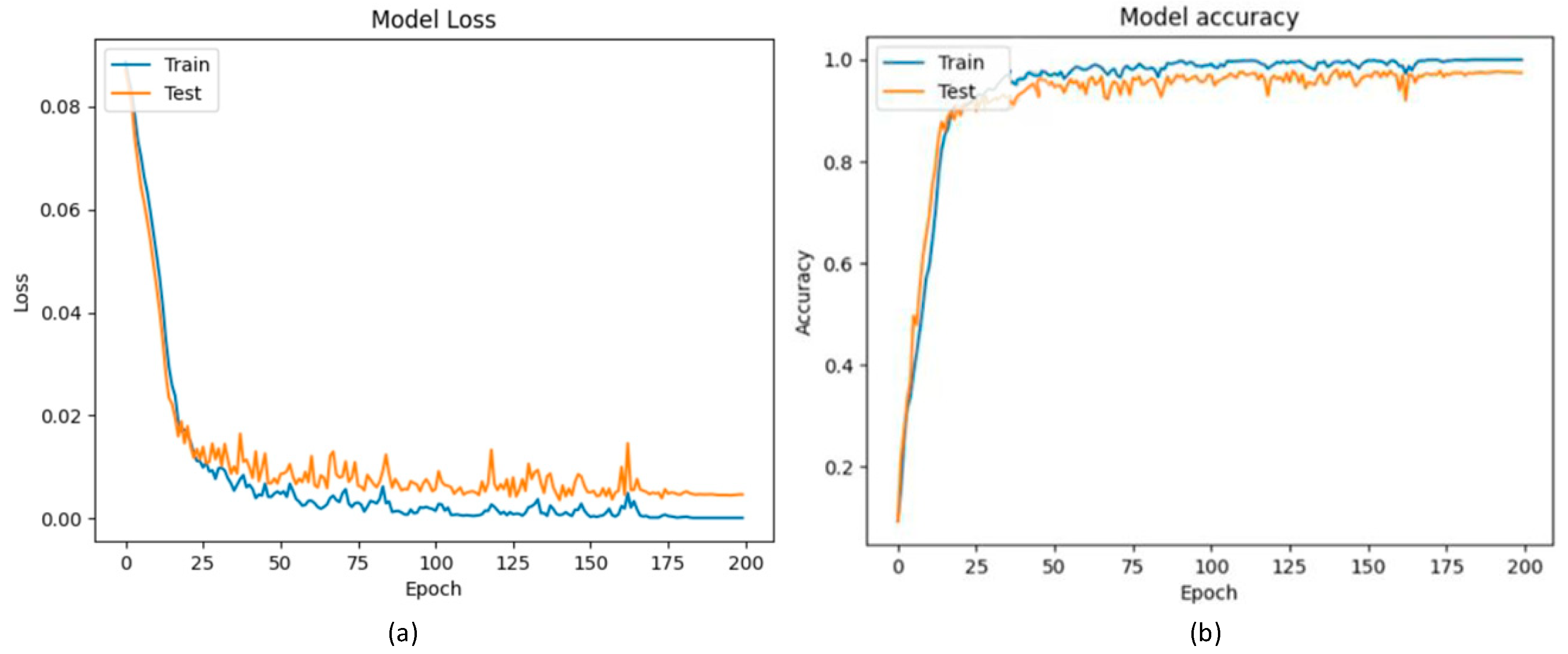
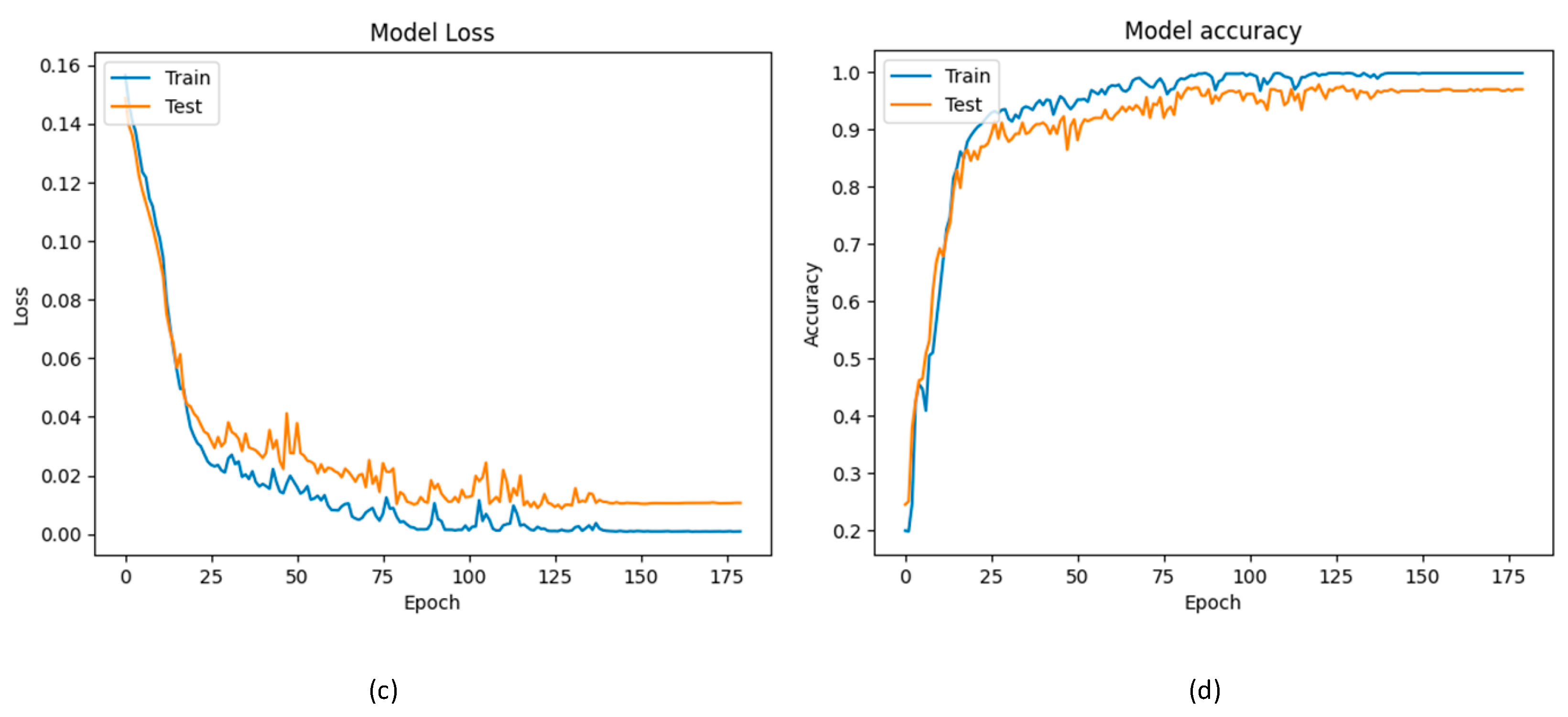
The two experimental results shown below are both the experimental results of the model on the test set, and using the Adam optimizer, the learning rate is 0.0001 and the batch size is 120. Figure 10a,b illustrate the CWRU dataset experiments’ accuracy and loss variations, while Figure 10c,d display those for the trials using a dataset gathered in a laboratory. The Y-axis in the figure represents the loss value of the model, which is used to evaluate the performance of the model. The x axis represents the number of iterations carried out in the experiment, which is used to reflect the convergence rate of the model. The experiment on the CWRU dataset underwent 200 iterations of training, while the laboratory-collected data experiment underwent 180 iterations of training. The loss function in both experiments was mean square error, or MSE, where a smaller loss value indicates a closer prediction to the actual values and better model performance. As observed in Figure 10a, the loss curve shows a rapid decline in the early stages of training and stabilizes after 175 iterations, as the test dataset loss approaches 0.01 and the training dataset loss approaches 0. According to Figure 10b, the accuracy curve shows the model achieving a final accuracy rate of 98.89%. In Figure 10c, the loss curve indicates a similar rapid decline in loss during the initial training stages, stabilizing after 120 iterations, the loss approaching 0 on the training dataset and less than 0.02 on the test dataset. The model achieves an accuracy rate of 96.70%, as indicated by the accuracy curve.

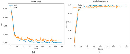
Figure 10. Loss function and accuracy curve plot. (a) The CWRU dataset’s loss variation; (b) the CWRU dataset’s accuracy; (c) the laboratory-collected dataset’s loss variation; (d) the laboratory-collected dataset’s accuracy.

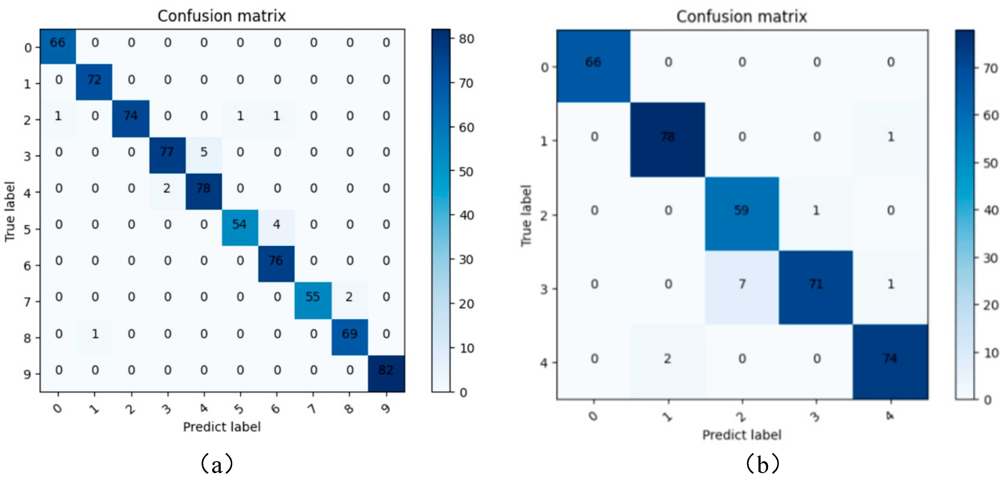
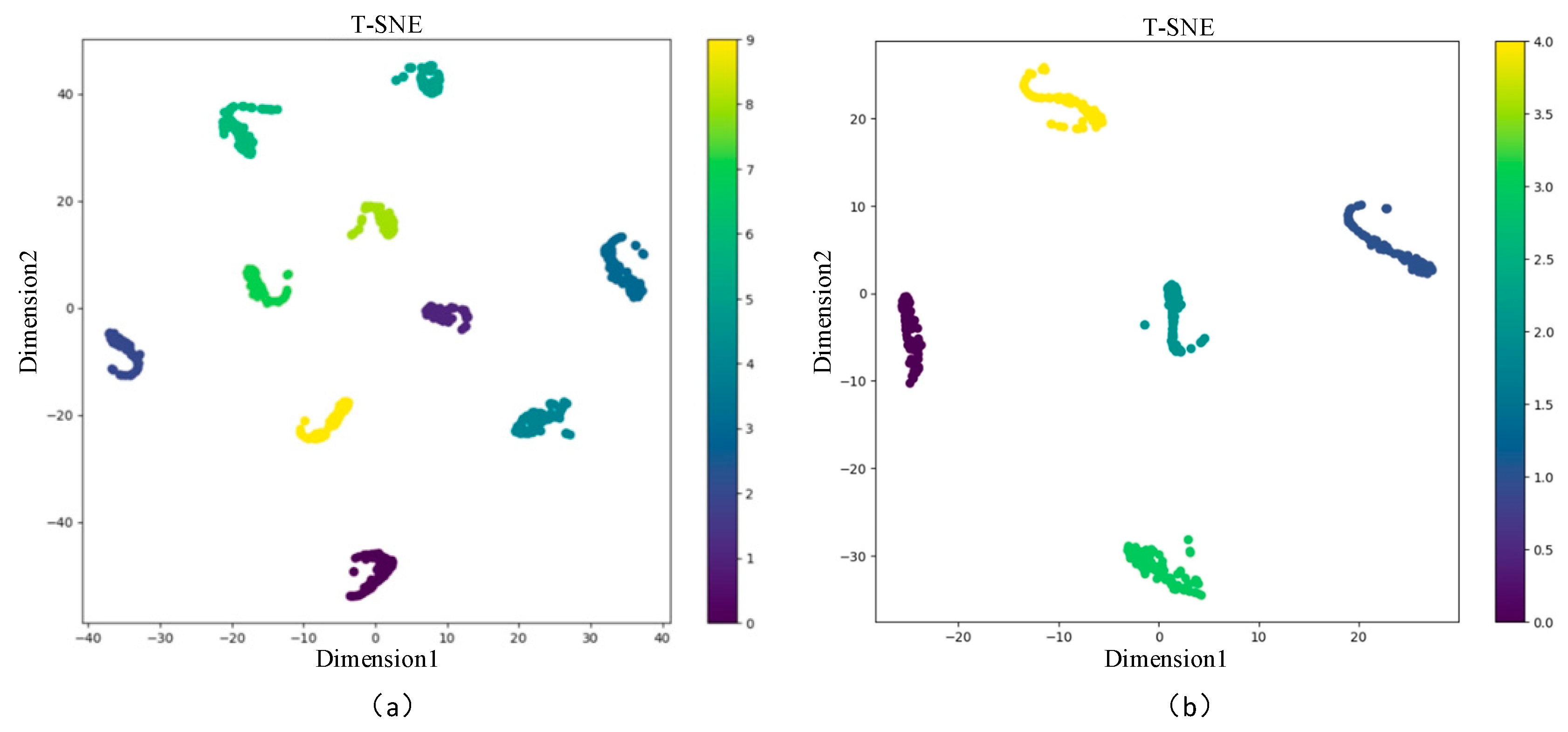
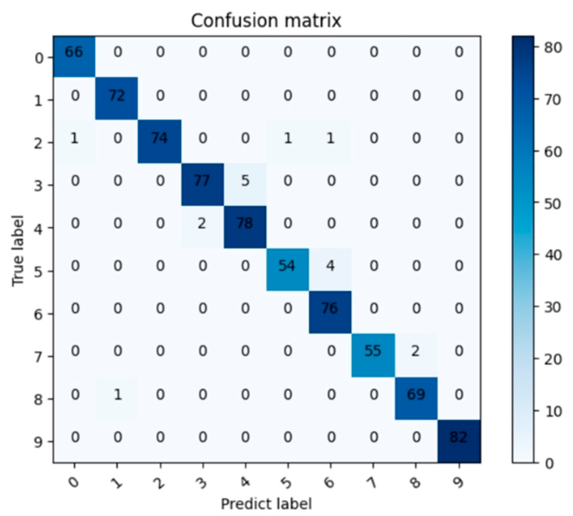
To visually assess the classification performance and overall model effectiveness, confusion matrices and t-SNE visualization techniques were employed, as depicted in Figure 11 and Figure 12. The pictures demonstrate the model’s exceptional performance on the laboratory-collected dataset as well as the CWRU dataset.

Figure 11. Confusion matrix. (a) The CWRU dataset’s confusion matrix; (b) the laboratory-collected dataset’s confusion matrix.

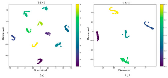
Figure 12. t-SNE visualization. (a) CWRU dataset’s visualization; (b) laboratory-collected dataset’s visualization.

4.3.2. Model Comparison

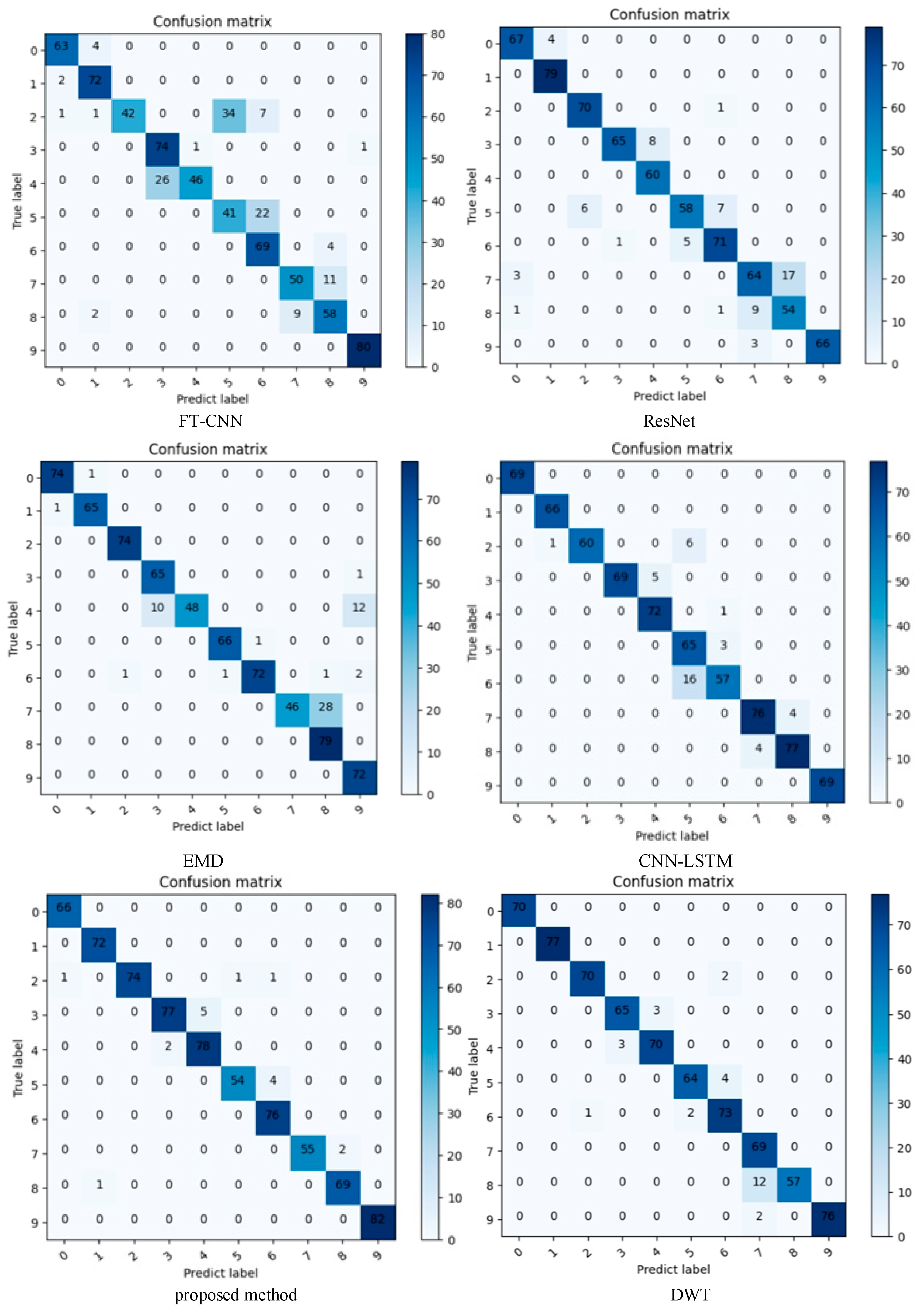
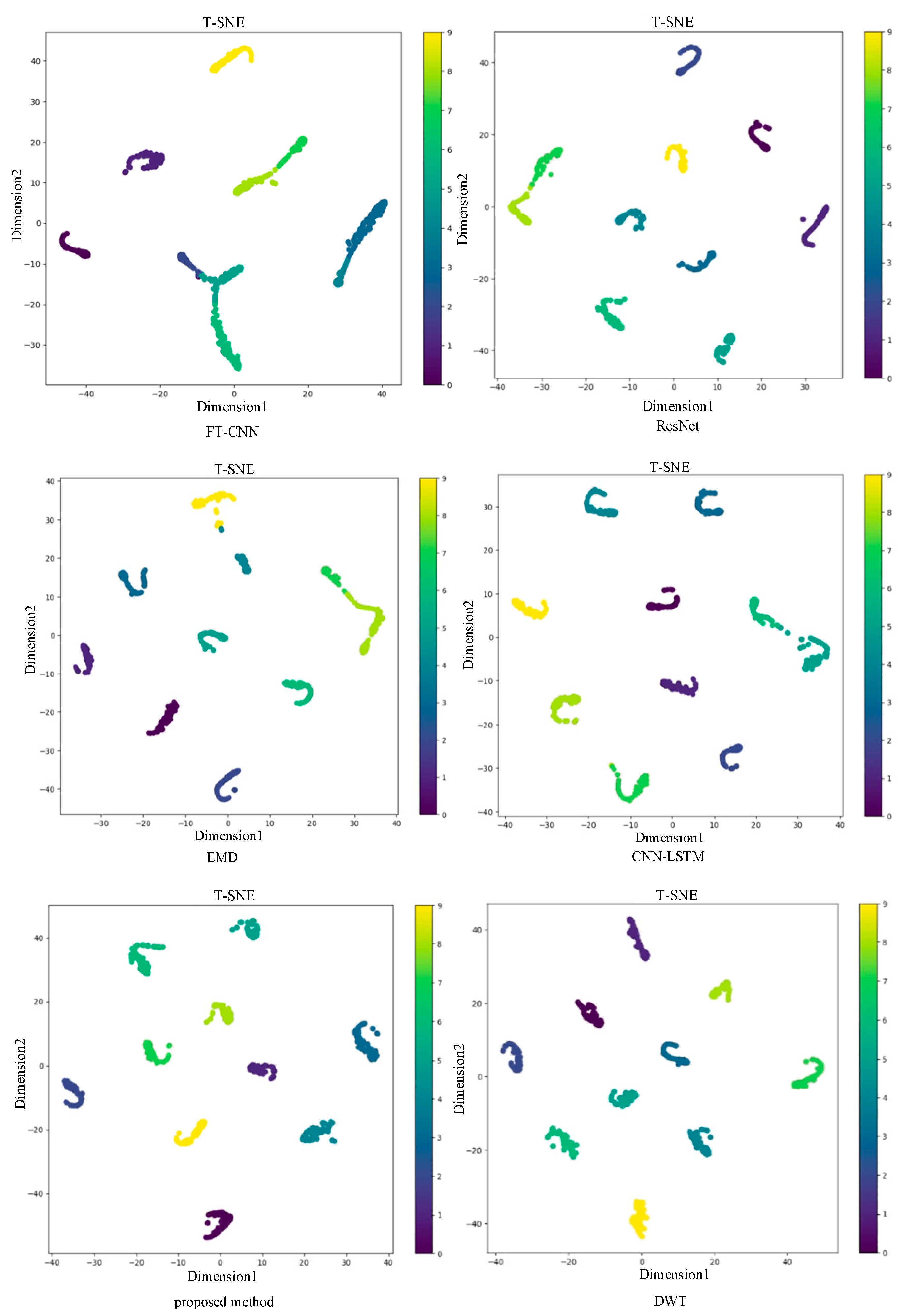
For ease of understanding and illustration, model comparisons and result analyses are conducted using the CWRU bearing dataset as an example. The study utilized various classification algorithms and control trials to verify the efficacy of the suggested feature extraction technique. The proposed method was compared in terms of performance with ResNet [37] and Fourier Transform (FT), Discrete Wavelet Transform (DWT), traditional CNN-LSTM models, and Empirical Mode Decomposition (EMD) as feature extractors, using softmax as the classifier. The comparative experimental results are illustrated in the Figure 13 and Figure 14.

Figure 13. Confusion matrix comparison.

Figure 14. t-SNE visualization comparison.

In order to confirm the effectiveness of the suggested feature extraction technique, comparative experiments were conducted using both the KNN algorithm and softmax algorithm. The results are shown in Table 4.

Table 4. Accuracy comparison.

Classification Algorithm	Feature Extraction Algorithm	Accuracy
Softmax	ResNet	91.30%
	CNN-LSTM	94.26%
	FT-CNN	92.66%
	EMD	86.08%
	DWT	96.80%
	Proposed method	98.89%
KNN	ResNet	76.80%
	CNN-LSTM	79.23%
	FT-CNN	77.80%
	EMD	73.62%
	DWT	81.23%
	Proposed method	83.8%

It is evident from the experimental findings and tables that the Empirical Mode Decomposition (EMD) has low accuracy due to the impact of mode mixing on the accuracy of signal decomposition. On the other hand, the frequency-domain CNN transforms signals into two-dimensional spectrograms through methods like Fourier Transform (FT) before utilizing CNN for feature extraction. However, this transformation process may result in the loss of important data, leading to relatively low recognition accuracy of the frequency-domain CNN. The accuracy of Discrete Wavelet Transform (DWT) is relatively high, but it decomposes the signal at a specific scale, which may result in a loss of detailed information. This work proposes a method that extracts feature information from many scales simultaneously by using multiple independent structures and then fuses the retrieved features, enabling a more comprehensive learning of data features. The suggested approach’s superiority has been confirmed by comparison with other categorization algorithms.

At the same time, we also compare the algorithm with the latest methods using the CWRU dataset. According to [38], the fault diagnosis method based on unsupervised features proposed in this article categorizes the CWRU dataset into four types of faults: normal, inner ring fault, outer ring fault, and rolling element fault; and it has an accuracy of 97.489% on the test dataset. The SSA-1DCNN-SVM proposed in [39] divides the CWRU dataset into six fault states: normal, rolling element fault, inner circle fault, 3 o’clock outer circle fault, 6 o’clock outer circle fault, and 12 o’clock method outer circle fault. The accuracy rate was 96.39%. The accuracy of both methods is lower than that of the proposed methods.

4.3.3. Analysis of Experimental Results

As shown in the Figure 15, it displays the classification outcomes of the approach that are suggested in this research. The predicted value labels are shown by the horizontal axis, and the true value labels are represented by the vertical axis. Among them, the accuracy rates for labels 0, 1, 6, and 9 are 100%, whereas the accuracy rates for labels 3 and 5 are relatively low. This could be attributed to the similarity of these signals in noisy environments, making them difficult to distinguish.

Figure 15. Confusion matrix.

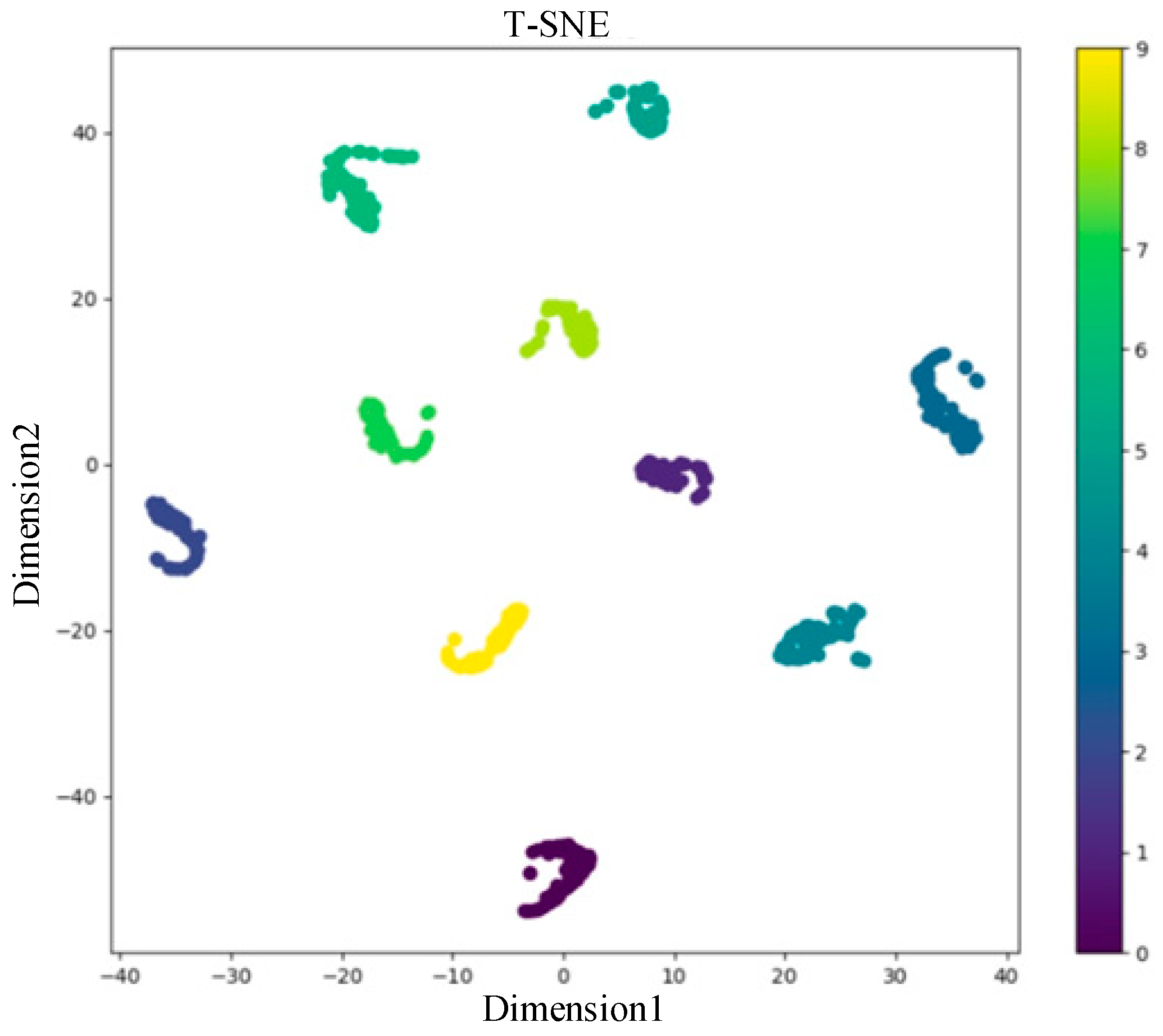
In order to assess the model’s performance even more, F1 scores, precision, and recall were used. The model’s performance metrics for each class are presented in Table 5: averaging 98% for F1 score, average accuracy, and average recall across all classes is what the model accomplishes. Additionally, the t-SNE algorithm was utilized for visualizing the classification results.

$$Precision={\displaystyle \frac{TP}{TP+FP}}$$

(8)

$$Recall={\displaystyle \frac{TP}{TP+FN}}$$

(9)

$$F1=2\times {\displaystyle \frac{Precision\times Recall}{Precision+Recall}}$$

(10)

Table 5. Specific condition.

	Unsupervised Features	SSA-1DCNN-SVM	Proposed
Motor speed	1750 rpm	1750 rpm	1750 rpm
Load	3 HP	3 HP	3 HP
Fault category	4	6	10
Accuracy	97.489%	96.39%	98.89%

In the formula, the definitions of TP (True Positive), FP (False Positive), and FN (False Negative) are indicated as shown in the Table 6.

Table 6. Result classes.

	Predicted Positive	Predicted Negative
Actual positive	True Positive (TP)	False Negative (FN)
Actual negative	False Positive (FP)	True Negative (TN)

Table 7 shows the accuracy, recall, and F1 score of each label, indicating that the model has high recognition accuracy for each type of fault.

Table 7. Evaluation metrics.

Label	Precision	Recall	F1 Score
0	0.99	1.00	0.99
1	0.99	1.00	0.99
2	1.00	0.96	0.98
3	0.97	0.94	0.96
4	0.97	0.97	0.96
5	0.98	0.93	0.96
6	0.94	1.00	0.97
7	1.00	0.96	0.98
8	0.97	0.99	0.98
9	1.00	1.00	1.00

Figure 16 illustrates clear boundaries between categories, indicating the effective differentiation of data points across different classes. The close clustering of points of the same color further demonstrates the model’s good classification performance.

Figure 16. t-SNE visualization.

4.4. Comparative Experiment

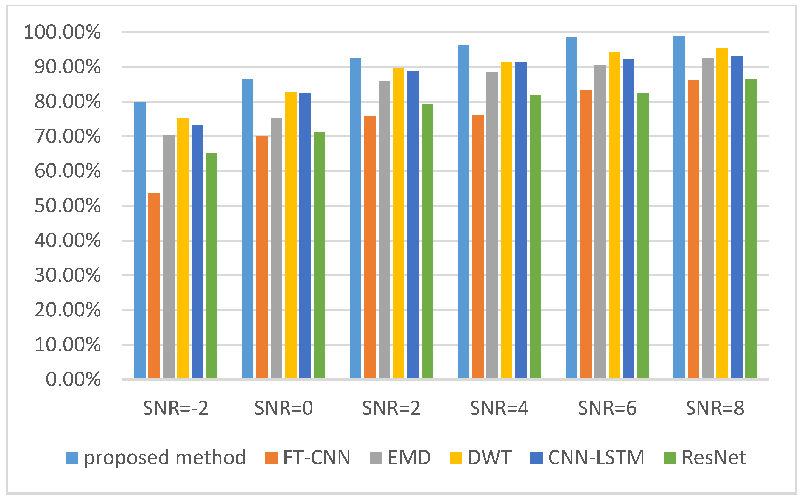
In the actual operation of tractors, there is noise in addition to the initial vibration signals. Therefore, the initial vibration signals were combined with Gaussian white noise using the following precise formula to test the effectiveness of the suggested method in noisy situations.

$$SNR=10{\mathit{log}}_{10}{\displaystyle \frac{P_s}{P_n}}$$

(11)

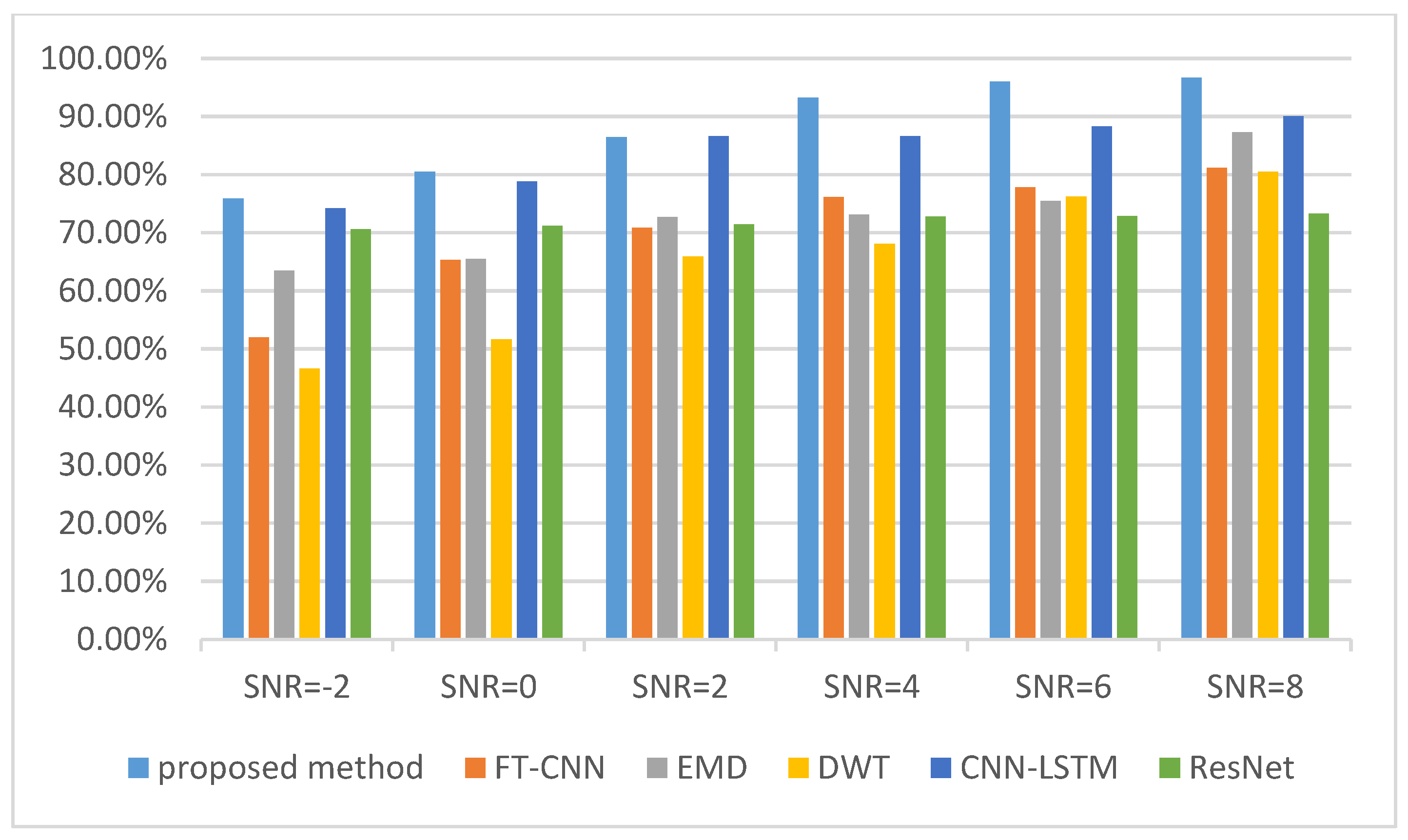
In the equation, SNR represents the ratio of signal to noise; the effective power of the signal is denoted by $P_s$; whereas the effective power of the noise is represented by $P_n$. When SNR is positive, it indicates that the signal power is greater than the noise power, whereas when SNR is negative, it signifies that there is a lower signal power than noise power. Noise ranging from −2 to 8 dB was added to the original vibration signals for model experimentation, with the softmax classification algorithm selected. The experimental outcomes are displayed in Figure 17 and Figure 18. It is evident that the suggested approach functions effectively even in noisy settings.

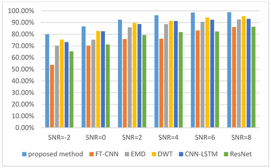
Figure 17. The accuracy variation in the CWRU bearing dataset in noisy environments.

Figure 18. The accuracy variation in the laboratory-collected gearbox data under noisy conditions.

4.5. Comparative Experiment

Ablation experiments were carried out to confirm the effect of various modules on the model’s performance. Three experiments were conducted in total, including removing the multi-head attention mechanism while retaining the adaptive soft threshold module, removing the adaptive soft threshold module, and removing both modules. Each module in the suggested strategy has an effect on the model’s overall performance, as demonstrated by the experimental results displayed in the Table 8. These modules, when used in combination, optimize the model performance.

Table 8. Results of the differential experiment.

Dataset	Differential Experimentation	Accuracy
CWRU bearing dataset	Remove multi-head attention	93.19%
	Remove adaptive soft threshold	95.42%
	Remove both	91.11%
	Proposed method	98.89%
Collected gear dataset	Remove multi-head attention	90.86%
	Remove adaptive soft threshold	90.10%
	Remove both	88.64%
	Proposed method	96.70%

5. Discussion

This method integrates the feature extraction capabilities of CNN, multi-head attention mechanism, and adaptive soft threshold. And in the experiment, it showed excellent feature extraction and fault identification performance. Its advantages include the following: (1) Multiple parallel 1D CNN networks are employed, which can extract and learn feature information from different scales, providing a more comprehensive understanding of the data. Additionally, these networks can directly utilize sequential data as input without the need for complex data preprocessing, thereby enhancing efficiency. (2) The use of a multi-head attention mechanism and a soft thresholding module helps to reduce the impact of noise and enhances the ability to understand features. In conjunction with a bidirectional long short-term memory network, this allows for global feature learning, which in turn improves the performance of the model. (3) Compared to other methods, it achieves higher accuracy and is capable of effectively identifying various types of faults.

However, this method also has certain limitations. The performance of the model may rely on high-quality and sufficient training data; if the training is biased, the diagnostic performance of the model will decrease. In future research, we will delve into this issue within the field of fault diagnosis, aiming to optimize the network structure. By considering the actual working environment of tractors, we will improve the efficiency of feature extraction and recognition accuracy of the network structure, while also enhancing the model’s applicability. Overall, these findings suggest that this method could be an effective tool for the fault diagnosis of tractor transmission systems.

6. Conclusions

In this study, a CNN-BILSTM-based fault diagnostic technique for tractor transmission systems is proposed, which innovatively integrates multiple algorithms to construct a novel multi-scale feature extraction approach.

Initially, raw vibration signals with different characteristics are fed into the network, processed by three different-scale feature extractors. The introduction of the multi-head attention mechanism and adaptive soft thresholding helps to better extract features by eliminating the influence of noise. Subsequently, the learned data undergo feature fusion module processing and are input into the BILSTM network to enhance the understanding of the fused data. Finally, to identify and categorize faults, the data are fed into the classification network.

The experimental findings show that, using the CWRU bearing dataset, the defect diagnostic accuracy was 98.89%. Furthermore, the accuracy of failure diagnosis utilizing the gearbox data gathered in the laboratory eventually reached 96.70%, and it also exhibited better performance in noisy environments compared to other models, proving the ability of the suggested method to conduct high-precision fault diagnostics.

References

- Wang, X. Analysis of Key Technologies for Maintenance and Repair of Tractors and Combine Harvesters. South Agric. Mach. 2022, 53, 153–155. [Google Scholar]
- Wang, Y.K.; Kang, L.F. Fault diagnosis of tractor bearings based on IoT and convolutional neural networks. J. Agric. Mech. Res. 2023, 45, 245–249. [Google Scholar]
- Chunhong, D. Briefly describe the key technologies of tractor transmission system. Tract. Farm Transp. 2022, 49, 9–13. [Google Scholar]
- Shichun, C. Research status of tractor variable speed transmission system technology. Agric. Technol. Equip. 2022, 06, 40–42. [Google Scholar]
- Guifen, R. Review of mechanical fault diagnosis techniques. Agric. Equip. Veh. Eng. 2021, 59, 69–73. [Google Scholar]
- Sepulveda, N.E.; Sinha, J. Two-step vibration-based machine learning model for the fault detection and diagnosis in rotating machine and its blind application. Struct. Health Monit. 2024. [Google Scholar] [CrossRef]
- Matania, O.; Dattner, I.; Bortman, J.; Kenett, R.S.; Parmet, Y. A systematic literature review of deep learning for vibration-based fault diagnosis of critical rotating machinery: Limitations and challenges. J. Sound Vib. 2024, 590, 118562. [Google Scholar] [CrossRef]
- Gangsar, P.; Bajpei, A.R.; Porwal, R. A review on deep learning based condition monitoring and fault diagnosis of rotating machinery. Noise Vib. Worldw. 2022, 53, 550–578. [Google Scholar] [CrossRef]
- Feng, K.; Yang, R.; Wei, Z. An optimized Laplacian of Gaussian filter using improved sparrow search algorithm for bearing fault extraction. Meas. Sci. Technol. 2024, 35, 036105. [Google Scholar] [CrossRef]
- Wang, M.; Yang, Y.; Wei, L.; Li, Y. A lightweight gear fault diagnosis method based on attention mechanism and multilayer fusion network. IEEE Trans. Instrum. Meas. 2024, 73, 3503011. [Google Scholar] [CrossRef]
- Nacer, S.M.; Nadia, B.; Abdelghani, R.; Mohamed, B. A novel method for bearing fault diagnosis based on BiLSTM neural networks. Int. J. Adv. Manuf. Technol. 2023, 125, 1477–1492. [Google Scholar] [CrossRef]
- Guo, Y.; Mao, J.; Zhao, M. Rolling Bearing Fault Diagnosis Method Based on Attention CNN and BiLSTM Network. Neural Process. Lett. 2023, 55, 3377–3410. [Google Scholar] [CrossRef]
- Zhang, X. Deep learning-based multi-focus image fusion: A survey and a comparative study. IEEE Trans Pattern Anal. Mach. Intell. 2022, 44, 4819–4838. [Google Scholar] [CrossRef] [PubMed]
- Vinodkumar, P.K.; Karabulut, D.; Avots, E.; Ozcinar, C.; Anbarjafari, G. A survey on deep learning based segmentation, detection, and classification for 3D point clouds. Entropy 2023, 25, 635. [Google Scholar] [CrossRef] [PubMed]
- Haque, S.; Eberhart, Z.; Bansal, A.; McMillan, C. Semantic similarity metrics for evaluating source code summarization. In Proceedings of the IEEE International Conference on Program Comprehension, Virtual Event, 16–17 May 2022; pp. 36–47. [Google Scholar]
- Hamdi, S.; Oussalah, M.; Moussaoui, A.; Saidi, M. Attention-based hybrid CNN-LSTM and spectral data augmentation for COVID-19 diagnosis from cough sound. J. Intelligent. Inf. Syst. 2022, 59, 367–389. [Google Scholar] [CrossRef] [PubMed]
- Zhang, X.; Wang, Y.; Wei, S.; Zhou, Y.; Jia, L. Multi-scale deep residual shrinkage networks with a hybrid attention mechanism for rolling bearing fault diagnosis. J. Instrum. 2024, 19, P05015. [Google Scholar] [CrossRef]
- Zhang, S.; Sun, Y.; Dong, W.; You, S.; Liu, Y. Diagnosis of bearing fault signals based on empirical standard autoregressive power spectrum signal decomposition method. Meas. Sci. Technol. 2024, 35, 015010. [Google Scholar] [CrossRef]
- Ravikumar, K.N.; Yadav, A.; Kumar, H.; Gangadharan, K.V.; Narasimhadhan, A.V. Gearbox fault diagnosis based on multi-scale deep residual learning and stacked LSTM model. Meas. J. Int. Meas. Confed. 2021, 186, 110099. [Google Scholar] [CrossRef]
- Shafiq, M.; Gu, Z. Deep residual learning for image recognition: A survey. Appl. Sci. 2022, 12, 8972. [Google Scholar] [CrossRef]
- Guo, L.; Gu, X.; Yu, Y.; Duan, A.; Gao, H. An Analysis Method for Interpretability of Convolutional Neural Network in Bearing Fault Diagnosis. IEEE Trans. Instrum. Meas. 2024, 73, 3507012. [Google Scholar] [CrossRef]
- Hosseinpour-Zarnaq, M.; Omid, M.; Biabani-Aghdam, E. Fault diagnosis of tractor auxiliary gearbox using vibration analysis and random forest classifier. Inf. Process. Agric. 2022, 9, 60–67. [Google Scholar] [CrossRef]
- Rhodes, J.S.; Cutler, A.; Moon, K.R. Geometry- and accuracy-preserving random forest proximities. IEEE Trans. Pattern Anal. Mach. Intell. 2023, 45, 10947–10959. [Google Scholar] [CrossRef] [PubMed]
- Zhu, Z.; Yang, Y.; Wang, D.; Tian, X.; Chen, L.; Sun, X.; Cai, Y. Deep multi-layer perceptron-based evolutionary algorithm for dynamic multiobjective optimization. Complex Intell. Syst. 2022, 8, 5249–5264. [Google Scholar] [CrossRef]
- Luczak, D. Machine fault diagnosis through vibration analysis: Continuous wavelet transform with complex morlet wavelet and time-frequency RGB image recognition via convolutional neural network. Electronics 2024, 13, 452. [Google Scholar] [CrossRef]
- Gougam, F.; Afia, A.; Soualhi, A.; Touzout, W.; Rahmoune, C.; Benazzouz, D. Bearing faults classification using a new approach of signal processing combined with machine learning algorithms. J. Braz. Soc. Mech. Sci. Eng. 2024, 46, 65. [Google Scholar] [CrossRef]
- Łuczak, D. Data-Driven Machine Fault Diagnosis of Multisensor Vibration Data Using Synchrosqueezed Transform and Time-Frequency Image Recognition with Convolutional Neural Network. Electronics 2024, 13, 2411. [Google Scholar] [CrossRef]
- Gao, S.; Li, T.; Zhang, Y.; Pei, Z. Fault diagnosis method of rolling bearings based on adaptive modified CEEMD and 1DCNN model. ISA Trans. 2023, 140, 309–330. [Google Scholar] [CrossRef] [PubMed]
- Wang, H.; Liu, Z.; Peng, D. Understanding and learning discriminant features based on multiattention 1DCNN for wheelset bearing fault diagnosis. IEEE Trans. Ind. Inform. 2020, 16, 5735–5745. [Google Scholar] [CrossRef]
- Huang, S.; Tang, J.; Dai, J.; Wang, Y. Signal status recognition based on 1DCNN and its feature extraction mechanism analysis. Sensors 2019, 19, 2018. [Google Scholar] [CrossRef]
- Sun, H.; Zhao, S. Fault diagnosis for bearing based on 1DCNN and LSTM. Shock Vib. 2021, 2021, 1221462. [Google Scholar] [CrossRef]
- Chen, X.; Yang, R.; Xue, Y. Deep transfer learning for bearing fault diagnosis: A systematic review since 2016. IEEE Trans. Instrum. Meas. 2023, 72, 3508221. [Google Scholar] [CrossRef]
- Brauwers, G.; Frasincar, F. A general survey on attention mechanisms in deep learning. IEEE Trans. Knowl. Data Eng. 2023, 35, 3279–3298. [Google Scholar] [CrossRef]
- Zhao, M.; Zhong, S.; Fu, X.; Tang, B.; Pecht, M. Deep residual shrinkage networks for fault diagnosis. IEEE Trans. Ind. Inform. 2020, 16, 4681–4690. [Google Scholar] [CrossRef]
- Ramaswamy, S.L.; Chinnappan, J. Review on positional significance of LSTM and CNN in the multilayer deep neural architecture for efficient sentiment classification. J. Intell. Fuzzy Syst. 2023, 45, 6077–6105. [Google Scholar] [CrossRef]
- Neupane, D.; Seok, J. Bearing fault detection and diagnosis using case western reserve university dataset with deep learning approaches: A review. IEEE Access 2020, 8, 93155–93178. [Google Scholar] [CrossRef]
- Ajayi, O.G.; Olufade, O.O. Drone-Based Crop Type Identification with Convolutional Neural Networks: AN Evaluation of the Performance of Resnet Architectures. ISPRS Ann. Photogramm. Remote Sens. Spat. Inf. Sci. 2023, 10, 991–998. [Google Scholar] [CrossRef]
- Amarbayasgalan, T.; Ryu, K.H. Unsupervised Feature-Construction-Based Motor Fault Diagnosis. Sensors 2024, 24, 2978. [Google Scholar] [CrossRef]
- Wan, M.; Xiao, Y.; Zhang, J. Research on fault diagnosis of rolling bearing based on improved convolutional neural network with sparrow search algorithm. Rev. Sci. Instrum. 2024, 95, 045111. [Google Scholar] [CrossRef]
Disclaimer/Publisher’s Note: The statements, opinions and data contained in all publications are solely those of the individual author(s) and contributor(s) and not of MDPI and/or the editor(s). MDPI and/or the editor(s) disclaim responsibility for any injury to people or property resulting from any ideas, methods, instructions or products referred to in the content. |
© 2024 by the authors. Licensee MDPI, Basel, Switzerland. This article is an open access article distributed under the terms and conditions of the Creative Commons Attribution (CC BY) license (https://creativecommons.org/licenses/by/4.0/).