Abstract
In this article, a torsional adapter is designed and evaluated through the comparison of analytical, numerical, and experimental tools. The adapter converts a conventional tension–compression test machine for cyclic loading to a modified application of both force-controlled and displacement-controlled torsional loading. The mechanism ensures a uniform distribution of loading application on both sides of the specimen. The determination of the durability curve can therefore be consistently carried out by acknowledging the geometric relation between the displacement of the test rig and the strain on the specimen. However, friction and clearance in the mechanism joints can cause energy dissipation; therefore, a detailed evaluation of this effect is mandatory before the use of the adapter. Here, it is shown that, using the current version of the adapter, the energy dissipation during torsional testing can be measured and later successfully considered during the determination of the torsional cyclic curve. Future improvements of the adapter will involve the reduction of the friction between the components of the mechanism.
1. Introduction
The evaluation of machine elements is based on the knowledge of the response of the material to basic loading conditions and their combinations [1,2]. Insight into the characteristics of machine elements, such as dynamic strength, fatigue performance, the behaviour of the element after the damage has occurred, and the damage growth, is important during product design [3,4,5]. A detailed knowledge regarding the product characteristics also ensures balanced expectations between the manufacturer capabilities and customer requirements [6]. Four basic load states are usually considered during the characterisation of material, i.e., tension–compression, bending, shear, and torsion. Hence, various tests under these operating conditions or their combinations can be found in the literature. Torsional loading is usually carried out on its own, i.e., as pure torsion, or can be combined with bending, shear, and axial loads [7,8]. Ju et al. [9] presented the analysis of a torsional behaviour model for reinforced concrete (RC) members subjected to combined loads. The material parameters for analytical or numerical models to simulate the response of the material in the form of strains and stresses were determined using a special test machine. The most widespread test machines perform uniaxial tension–compression loading. Most of the conventional engineering materials and also emerging new materials are characterised by these tests to determine either their static or cyclic properties [10,11]. For example, in a study by Huang et al. [10], high-strength sorbite stainless steel S600E was examined using material tensile tests, axial compression stub column tests, and axial compression long column tests to determine the constitutive curves and failure patterns. In another recent study, Zhang et al. [12] inspected the influence of various welding methods and their influence on the fatigue properties of steel butt joints by means of cyclic tests. Similarly, Dong et al. [13] developed a cyclic loading test device and studied the cyclic tension–compression behaviour of AA7075-T6 under electrically assisted conditions.
Due to the rapid development of composite materials and complex shapes of mechanical components, multiaxial stress–strain responses will occur in machine elements during operation. Therefore, besides normal properties, shear properties need to be evaluated too. One option for the characterisation of the shear properties of engineering materials is through the utilisation of shear tests; for example, Yang et al. [14] carried out compression–shear tests for rock models with circular tunnels to analyse the shear failure mechanism of a rock tunnel. However, another option for the characterisation of the shear properties of engineering materials is through the utilisation of torsional tests [15,16]; for example, Malecka and Lagoda [17] used cyclic torsion to determine fatigue properties of RG7 bronze between 100,000 and 500,000 load cycles. Importantly, torsional test rigs are usually available in two versions—as either horizontal or vertical test rigs. The horizontal torsional test rigs usually load the specimen with pure or fixed torsion [17,18], whilst the vertical torsional test rigs combine the torsion with either tension or compression [19]. Fu et al. [20] designed a special micro tension–torsional fatigue testing apparatus for thin stent wires. Both pure torsion and tension–torsional fatigue tests can be performed by the apparatus [21]. Petit et al. [22] optimised an ultrasonic torsion fatigue system in order to increase the stress amplitude in the specimen and increase the robustness of the system; it was shown to be suitable for very high-cycle fatigue tests. Ogawa et al. [23] developed a test machine which can combine bending and torsion loading and perform fatigue tests at a high frequency under proportional and nonproportional loading conditions.
Instead of using a special torsional test rig, an existing uniaxial tension–compression test machine can be adapted to perform the torsional loading [24]. Recently, Goanta [25] developed a device used for torsion fatigue testing, which is adaptable to a universal pulsating testing machine and designed to determine the torsion fatigue limit for different materials. However, a general issue of torsional adapters is the appearance of friction during the experiment [26,27,28]. The friction mainly appears in sliding contacts—most commonly between bushings and rings—in bearings, or between the surfaces of mechanism connecting rods. On the contrary, disturbance can be brought into the experiment by clearance between the abovementioned mechanism components as a side effect of the attempt to reduce the friction. Huiyuan et al. [29] presented a contact analysis method for a large negative clearance four-point contact ball bearing. The results showed that a great effect on the contact stresses was made by tiny changes of the negative clearance. Therefore, both friction and clearance have to be evaluated prior to the utilisation of the torsional adapter. Tan et al. [30] presented the influence of the friction coefficient on the nonlinear dynamic characteristics of the mechanism with a clearance joint. They presented how friction could affect the acceleration levels of the mechanism and how it could play a positive role in the stability of the system.
The aim of this study was an upgrade of an existing test machine, commonly used for tension–compression loading, by developing an adapter for application of torsional loads. The main requirements for the adapter were (i) a deterministic conversion of tensile–compressive movement into torsional loading and (ii) measurement of the torsional stress–strain response. A friction model in the adapter hinges was sought for, both analytically and numerically. The analytical analysis involved the determination of displacement–rotation and force–moment connections between the parts prior to the friction evaluation. The numerical approach introduced a digital twin of the torsional adapter with a prior definition of the contacts between the mechanical parts and corresponding evaluation of the friction. Moreover, the digital twin supplied the calculation of the stress–strain response of the torsional specimen. Finally, the specimens were physically tested and then the comparison with the analytical and numerical solutions was made. Moreover, the experimental results served for the calibration of the digital twin.
2. Method
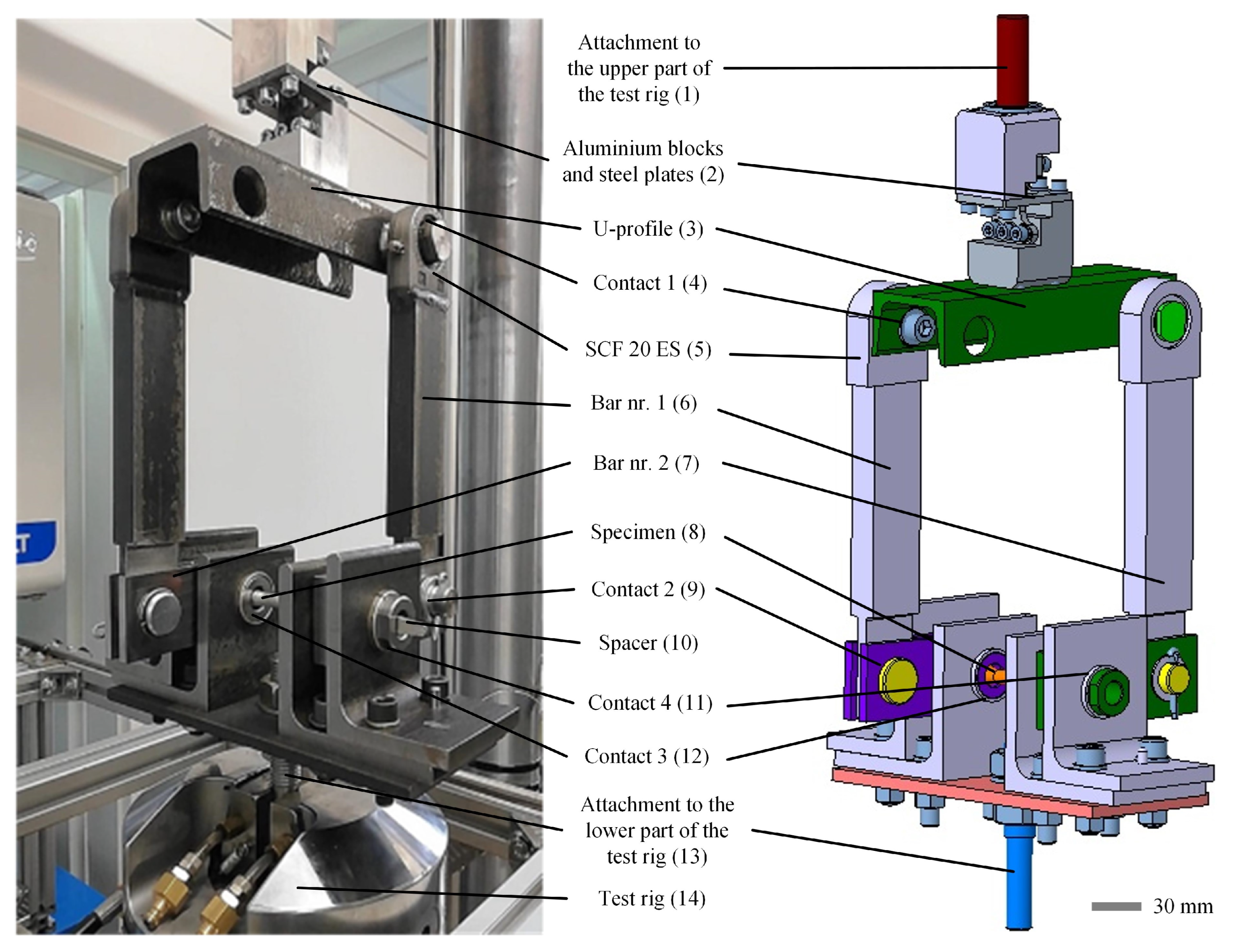
The adapter for torsional loading was designed for installation on an existing uniaxial tension–compression test rig (Figure 1). At the top, the adapter was tied to the test rig using two aluminium blocks and two steel plates (position 2 in Figure 1), which together formed a kinematic joint. The upper aluminium block was fixed to the upper clamp of test rig (1). The lower aluminium block was screwed to the U profile (3). Diagonally, two bushings were welded to the U profile for the connection of the vertical bars (6). The parts of the mechanism from the top attachment up to this point can only move in the vertical direction. Open profiles are in general not a good design solution for torsional loads due to low torsional stiffness. However, as the maximum torsional moment needed to load the specimen in this application was not high and the shape of the U profile represents an elegant solution to attach the vertical bars under 90° in initial position, the U profile as given in Figure 1, position 3, was chosen to perform the loading function. The sufficiency of the U profile was checked prior to the installation in the mechanism. The force transfer was continued using two bars (6) connected to the U profile by two pins. Every pin was tightened to the bushing by a bolt. The rotation between the pin and the bar was allowed, which was also the first analysed contact (4). The contact was performed using rod end bearing SCF 20 ES (5), which was welded to the top of bar nr. 1 (position 6). At the other side, bar nr. 1 is connected to bar nr. 2 (position 7) by a pin, which represented the second analysed contact of the mechanism (9). Bar nr. 2 was positioned using a bushing at the opposite side. The bushing was inserted into L supports, which were tightened to the base plate. The base plate was fixed to the lower side of the test rig (13). Contacts 3 and 4 (positions 11 and 12) analysed during the study can be found between the bushing’s outer diameter and bars nr. 1 and nr. 2, respectively. The same four contacts were examined on the other (symmetrical) half of the torsional adapter (Figure 1). A specimen was inserted through the inner diameter of the bushing. The fastening of the specimen (8) was completed using a screw notch. When the U profile was shifted vertically, bar nr. 1 rotated bar nr. 2, which then provided the torsional loading of the specimen.
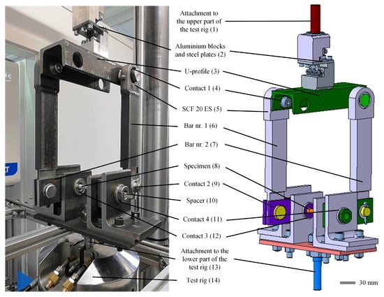
Figure 1.
Adapter for torsional loading: (left) physical product mounted onto to the tension–compression test rig and (right) digital twin used to carry out numerical simulations.
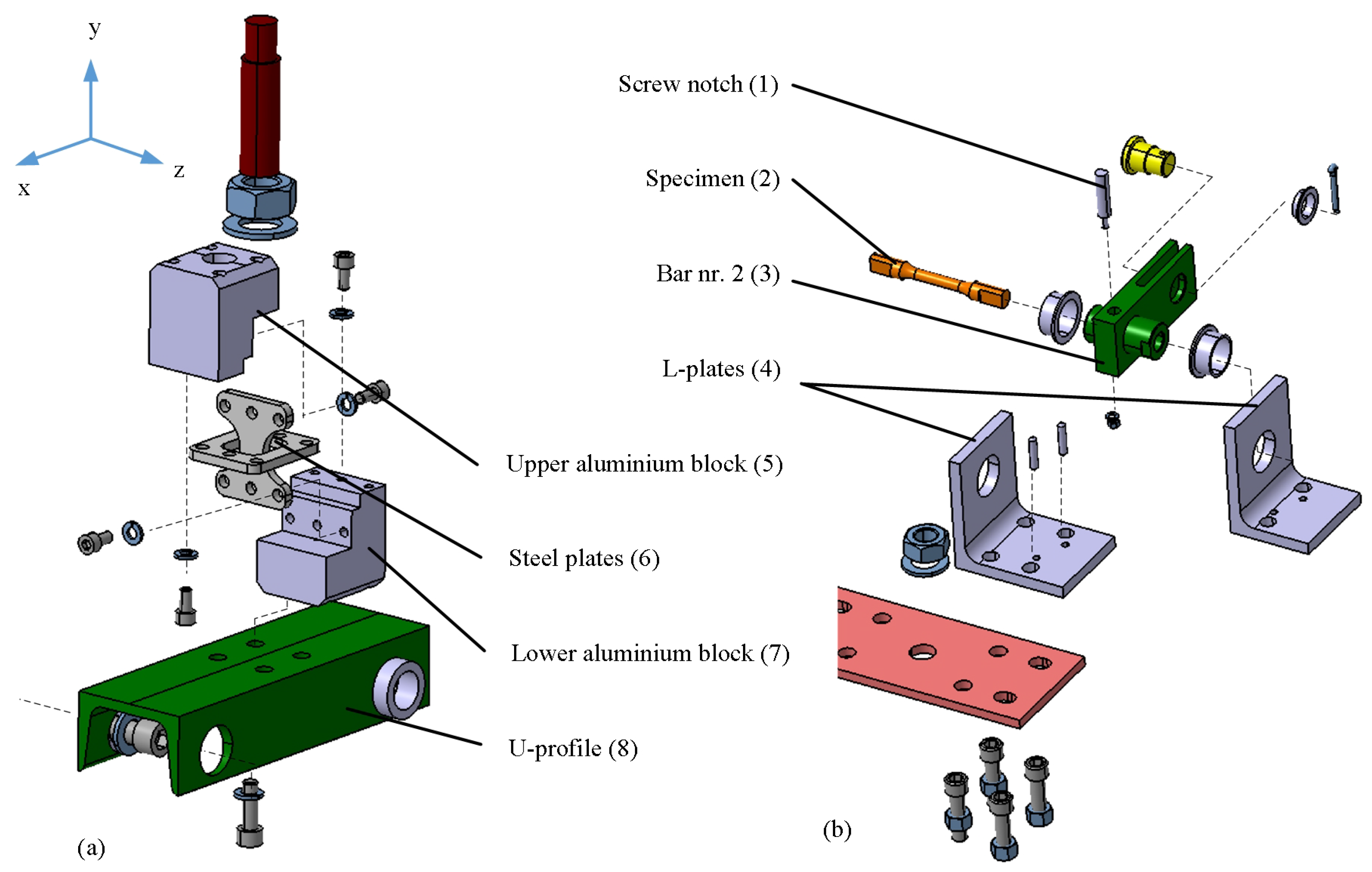
Furthermore, two details of the adapter are shown in Figure 2. The kinematic joint formed by the two aluminium blocks and two steel plates (positions 5, 6, and 7 in Figure 2) ensured an equal distribution of the loading to both sides of the mechanism, as the rotational rigidity of the joint is the smallest around its z axis. All other degrees of freedom (all translations and rotations around x and y axes) have a considerably higher stiffness, which then prevents the deformation in those directions. The fastening of the specimen, however, was ensured using a screw notch (position 1 in Figure 2), which created a fixed connection between the specimen (2) and bar nr. 2. (position 3). Bar nr. 2 was then inserted between two L plates (4), which created a rotational joint with sliding contacts. If the groove on the specimen is too loose for the screw notch to fix the specimen to bar nr. 2, an additional spacer can be inserted between the specimen and the screw notch to ensure a tight fit. An additional spacer can be seen in the physical form of the torsional adapter in Figure 1 at position 10.

Figure 2.
Details of the adapter for torsional loading: (a) the kinematic joint formed by two aluminium blocks and two steel plates and (b) the fastening of the specimen.
The torsional adapter was manufactured from steel S235. The specimen used in the study was made of aluminium alloy Al6061. The material properties are presented in Table 1 and were used in both the analytical and the numerical model.

Table 1.
Material properties of the parts of the torsional adapter.
2.1. Analytical Model
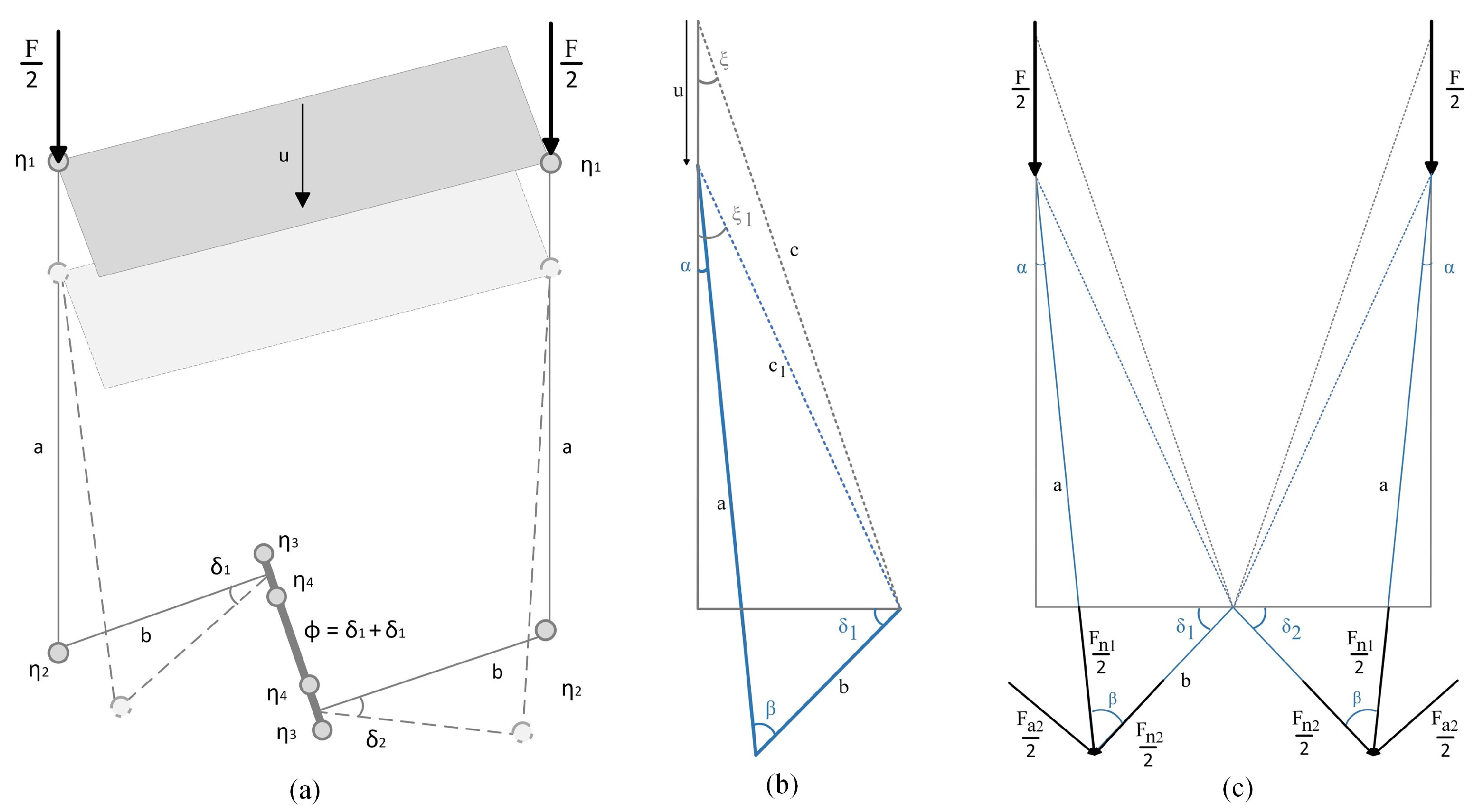
An analytical model considered both sides of the test rig. First, the connection between the vertical movement and the rotation of the specimen was established. The geometries of bars nr. 1 and nr. 2 are known and presented in Figure 3. The angles, when the mechanism is moved by a vertical shift u, are labelled as , , and . They are calculated using Equations (1)–(3):
and
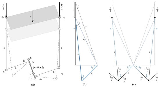
Figure 3.
Analytical model of the torsional adapter: (a) simplified sketch of mechanism; (b) angles between U profile, bar nr. 1 and bar nr. 2 on one half of the mechanism when it is moved downwards by a vertical shift u; (c) decomposed force F into normal and axial components with respect to bar nr. 1 considering contributions from both sides of the mechanism.
Angles and can be observed between bars nr. 1 and 2 when the mechanism is in the neutral position and shifted, respectively (Figure 3b).
The rotation of the specimen is defined as
Once the angle of rotation of the specimen is calculated, torsional moment can be calculated using Equation (5) as
where G stands for the shear modulus, is the torsional constant of the specimen cross-section, and L is the specimen gauge length. The torsional moment can also be defined according to Equation (6), where loading force rotates the bar nr. 2 at length b (Figure 3c). By calculating the equilibrium from the loading force F and rotations around angles and , the torsional moment can also be determined as
The normal force at length b can thus be expressed as
which, by determining Equation (6), yields
However, since the angle is usually very small, normal force can be approximated as
Considering the calculated angles , , and , the normal component of force and force F can be calculated using Equations (10) and (11), which are respectively defined as (Figure 3c).
and
Second, force F is decomposed into normal and axial components with respect to bar nr. 1 using Equations (12) and (13), which are respectively defined as
and
Components and provide the rotation of the mechanism, while components and generate friction in the contacts of the mechanism. Additionally, components on both sides of the torsional adapter create a rotating moment that is transmitted to the test rig at both attachments (positions 1 and 14 in Figure 1). The same moment is also transferred through the whole structure of the torsional adapter; therefore, zero clearance in the contacts is of crucial importance for a successful measurement during the torsional test. However, if the hydraulic piston to provide the loading is not designed to lock in rotation with respect to its own axis, the operation of the test machine could be damaged. The minimisation of this effect was hence considered during the design of the torsional adapter using the initial vertical positions of bar nr. 1 (position 5 in Figure 1). Enlarging the angle by attaching bar nr. 1 closer to the lower aluminium block (position 2 in Figure 1) on the U profile (position 3 in Figure 1) amplifies the rotating effect and potential damage to the test machine.
Two methods can be used to evaluate the friction force in the contacts. Following method 1, the friction force is calculated using Equation (14):
The friction coefficient is assumed constant in all contacts. Once the friction force is calculated, the work done by the friction force is calculated as
where r stands for the radius of the joint in the contact.
Furthermore, the total work of the system is calculated as the product of the force on the test rig F acting on the vertical bar nr. 1 and the displacement u:
The system losses can hence be represented as the total work due to the friction force compared to the work done by the force on the test rig:
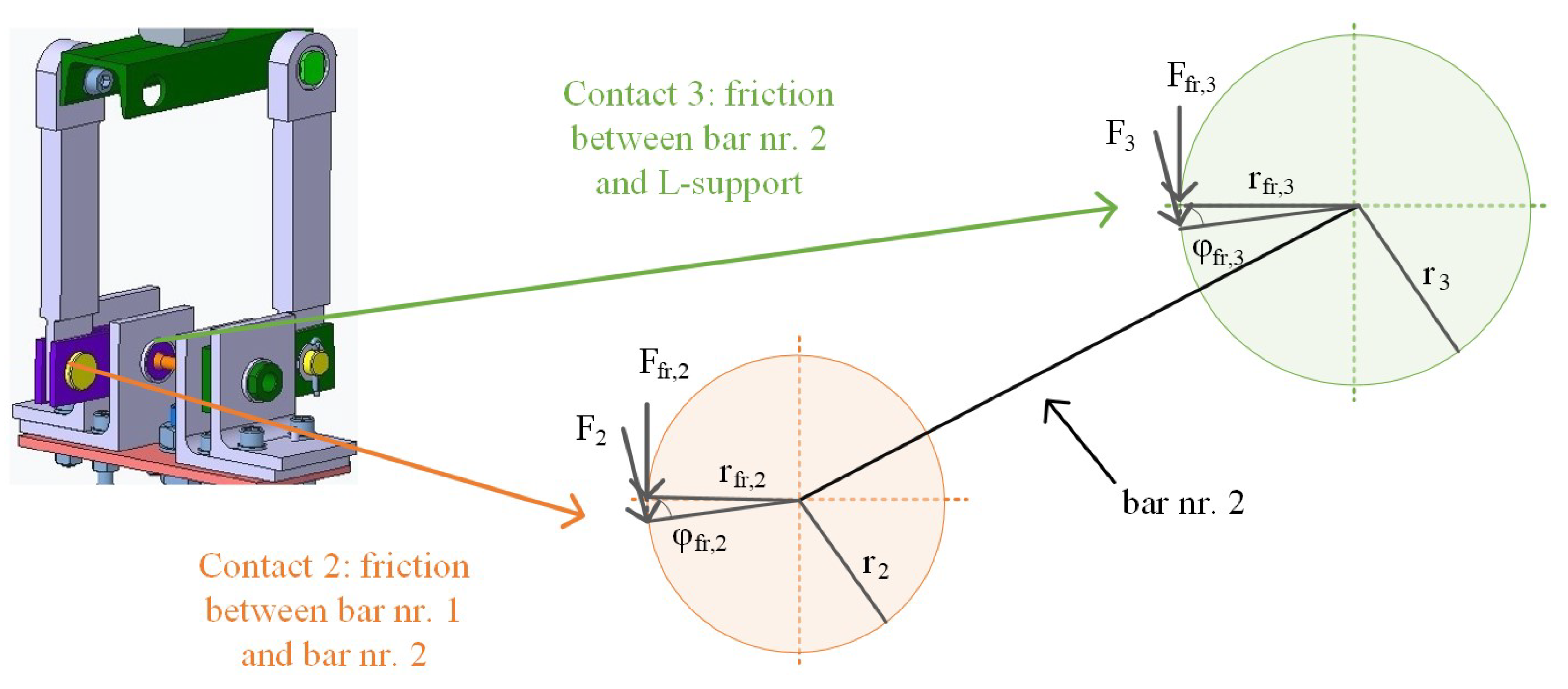
Following method 2, a part of the torsional moment is dissipated due to the friction in contacts 1–4. The dissipation is described by the friction moment . The analytical solution of the dissipation is based on the evaluation of the friction moment as defined by Benavides et al. [31]. The friction moment has to be calculated for the four contacts presented in Figure 1. Hence, beside the torsional moment , each friction moment caused by friction force must be introduced (Figure 4).

Figure 4.
Friction moment caused by friction force in contacts 2 and 3.
The friction angle is found between the friction force’s application point and the force (Figure 4). It is related to the coefficient of friction in the contact as defined by
The friction force is applied at the friction radius , which is defined as
where represents the radius of the grip of the loading force . The friction moment for a chosen contact is then expressed as
Compared to the total moment needed (Equation (5)), the sum of the friction moments represents the system losses:
2.2. Numerical Model
The numerical model was created in Abaqus/CAE. Two materials were used during the study: S235 steel and Al6061 aluminium alloy. Their material properties are given in Table 1. The model was meshed with 15,500 finite elements of type C3D8 and C3D6 sized between 2 and 5 mm. Steel was considered elastic during the numerical analysis, whereas the aluminium alloy was described using elastoplastic material properties. The plastic region was taken into account and determined using the Armstrong–Frederick model [32,33,34]:
where and represent the stress and the plastic strain in the constitutive elastoplastic material model of the aluminium alloy, respectively. The values of the material parameters for the Armstrong–Frederick model were determined according to the available data for the same material in [35]. They are presented in Table 2.
Table 2.
Parameters for Armstrong–Frederick material model of Al6061 aluminium alloy.
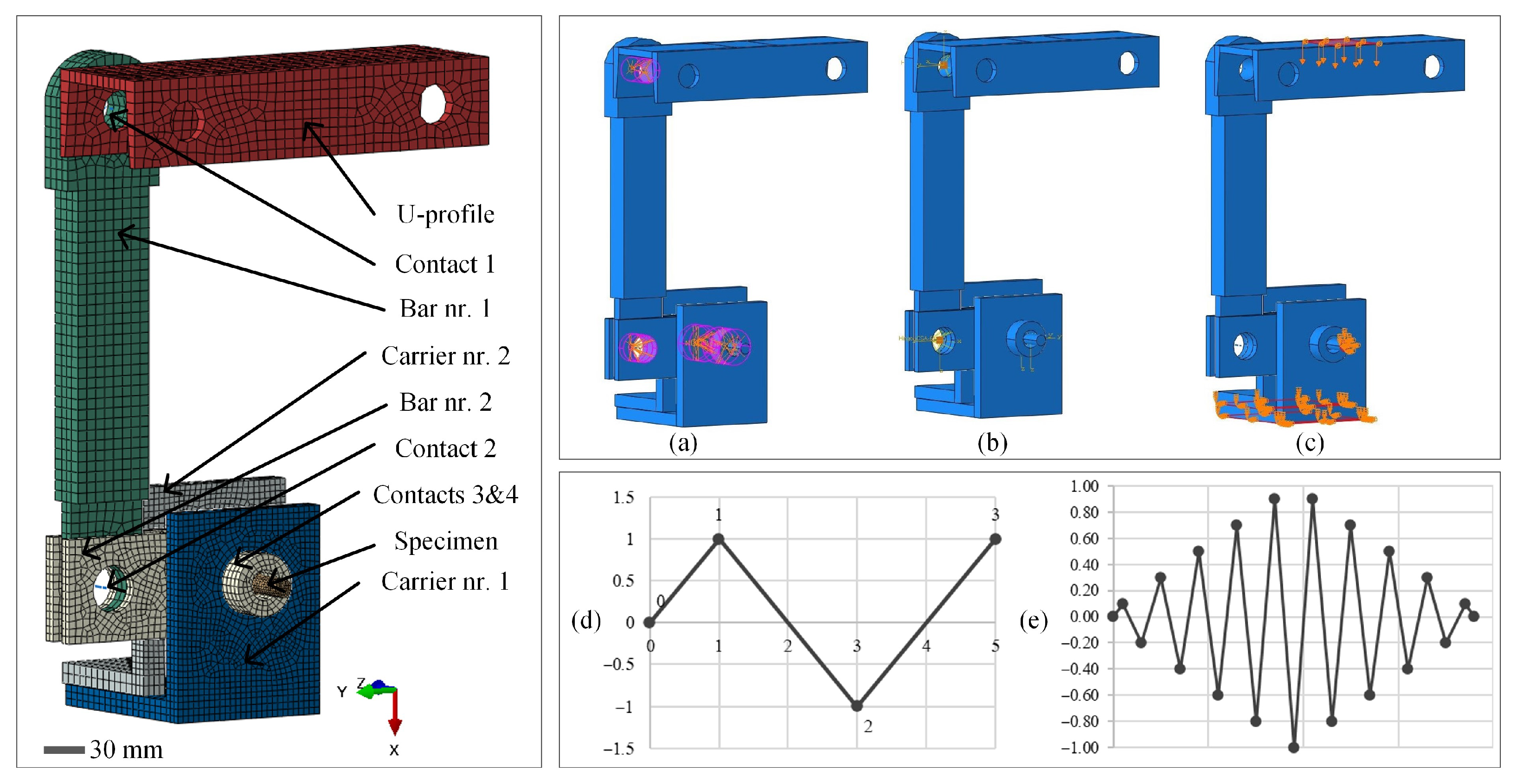
In Figure 5, the finite element mesh of both the torsional adapter in the neutral position and the specimen is given. The contact surfaces were connected to the reference points (Figure 5a). The reference points were then merged to create hinge connections (Figure 5b). The sliding conditions were set for the hinge connections either as frictionless or with friction. Both the boundary and the initial conditions were set as given in Figure 5c. Namely, the displacements and rotations were locked in all three directions on the lower surfaces of the both bars. The symmetry boundary condition was set in the midplane of the specimen to consider the other side of the torsional adapter in the simulation. The displacements in y and z directions at the top surface of the U profile were locked to allow for the vertical movement only. The simulation was controlled by the displacement of the U profile in the x direction. The loading signals for the low-cycle fatigue (LCF) and the incremental step test (IST) simulations are presented in Figure 5d and 5e, respectively.
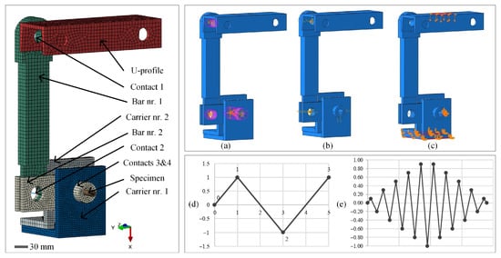
Figure 5.
Left: finite element mesh of the adapter in the neutral position and the specimen. Right: (a) reference points and couplings for contacts 1–4; (b) definition of hinge connections in contacts 1–4; (c) application of boundary conditions; (d) LCF load signal; and (e) IST load signal.
2.3. Experimental Procedure
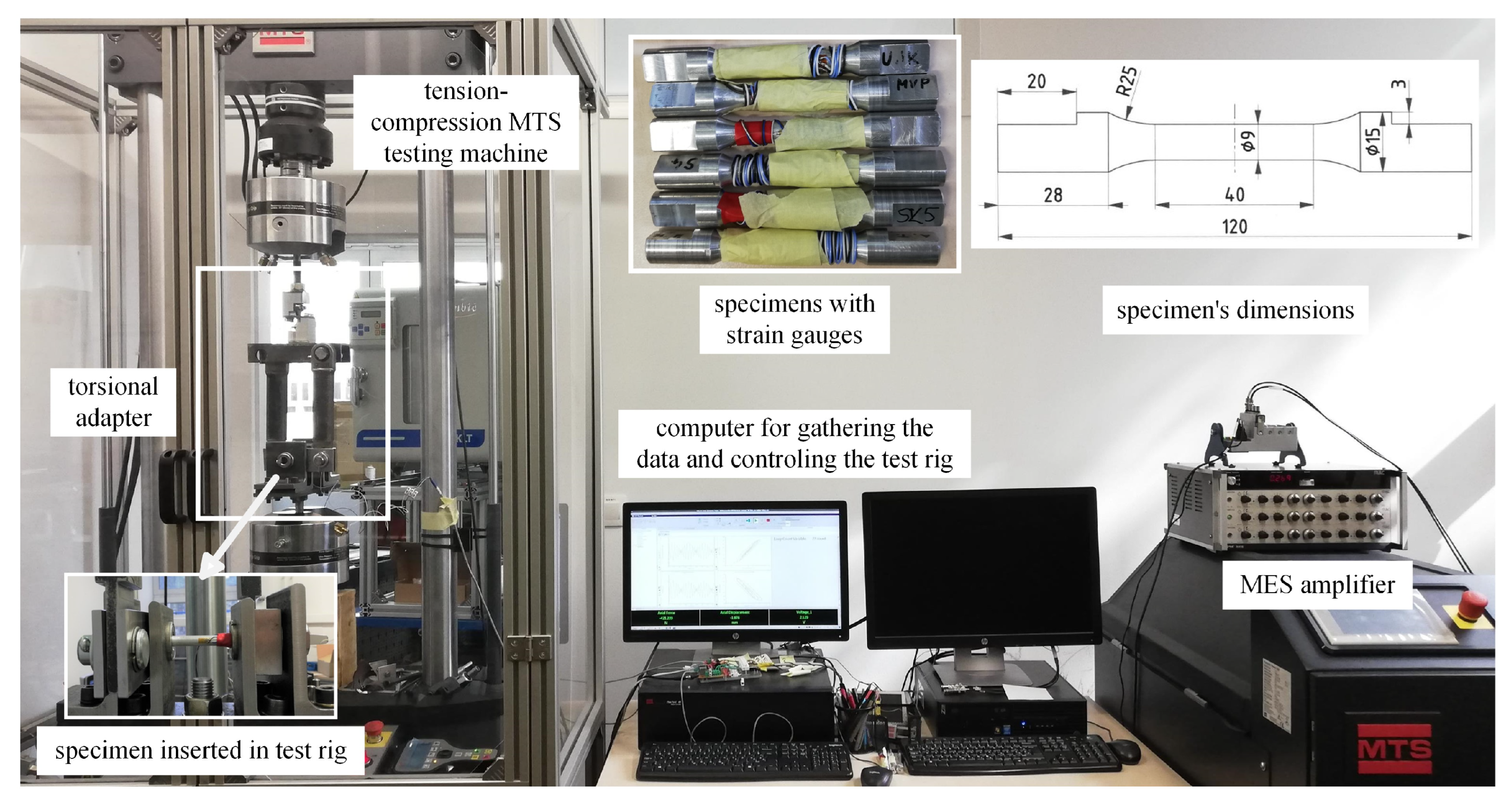
The torsional adapter was initially mounted to the tension–compression test machine as depicted in Figure 6. Next, a specimen with dimensions shown in Figure 6 was placed into the adapter. Two loading histories were prepared: LCF loading at several amplitudes and IST with a maximum displacement amplitude of 1 mm.
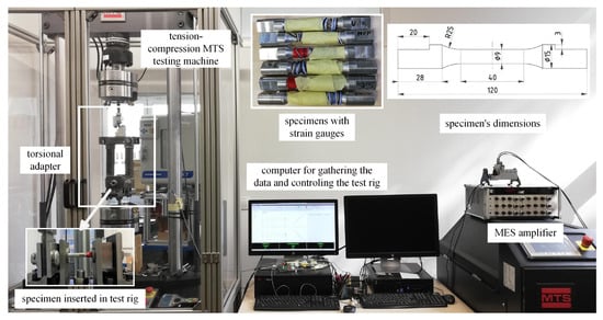
Figure 6.
Experimental setup and specimen dimensions.
Force and displacement were measured directly on the test rig. Additionally, a half bridge Wheatstone configuration for the measurement of the shear strains was applied to each of the specimens [36]. The reason for this was the search for the transfer function between the application of the displacement and the rotation of the specimen. Using the measurement of the bridge imbalance , the measured strains can be determined from
where and stand for the input voltage, output voltage, strain gauge constant, and the measured principal strain values, respectively [36]. Supposing that , Equation (23) can be simplified into
Engineering shear strain can finally be determined from the measured principal strain as
3. Results and Discussion
First, the results are separately presented for the analytical, numerical, and experimental evaluation. Afterwards, a correlation between the results is carried out.
3.1. Results of Analytical Model
The analytical solution is shown for the aluminium specimen. In Table 3, important measures for the analytical model are given. They correspond to the maximum analysed displacement of mm.
Table 3.
Geometric measures of the analytical model.
Based on the geometric and material properties of the specimen (Table 4), the torsional moment is calculated using Equation (26) as
Table 4.
Specimen properties used in the analytical model.
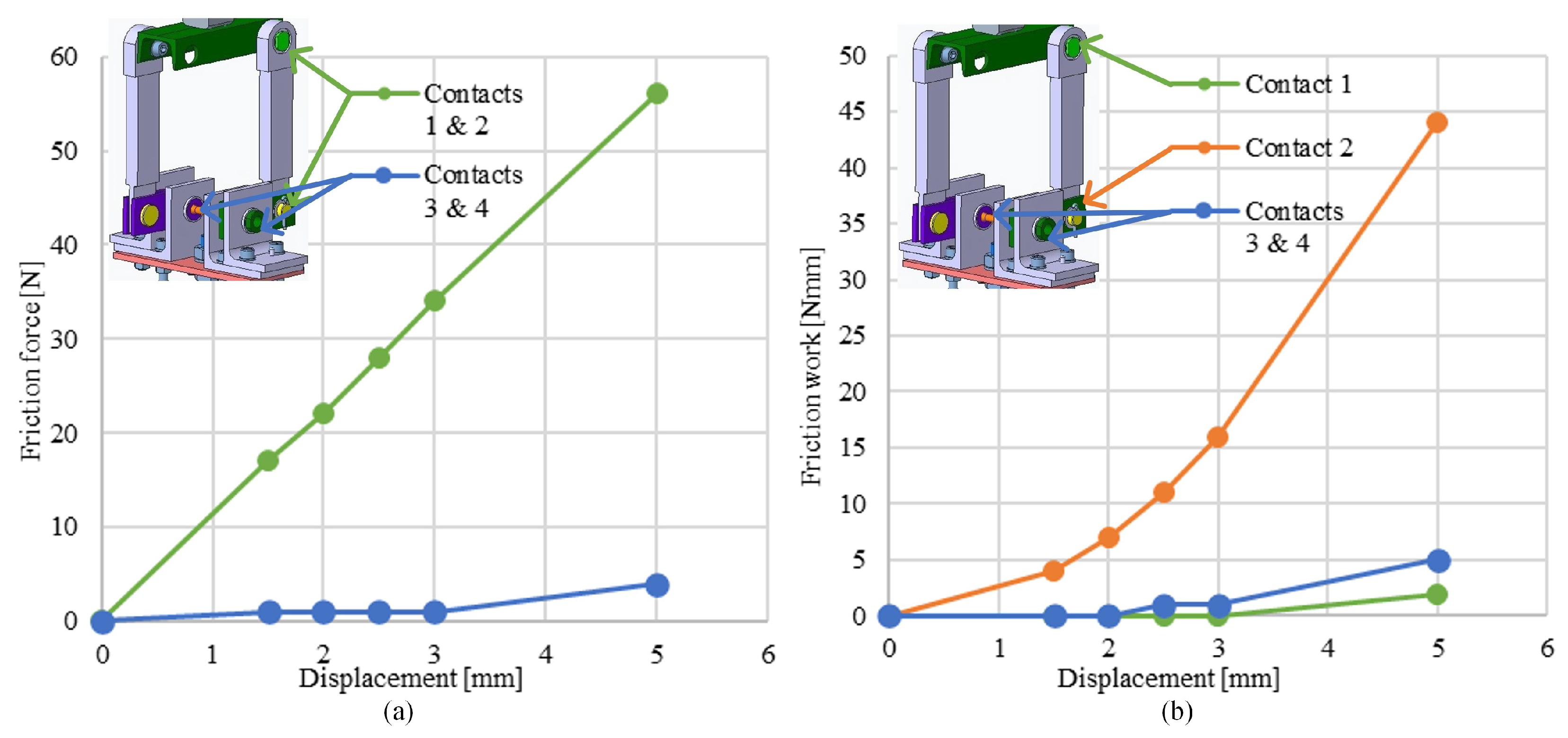
Following method 1 for determination of system losses, the friction forces in contacts 1–4 were calculated using Equations (9)–(14), with the coefficient of friction set to [37]. The results, including both sides of the mechanism, are given in Figure 7a. Moreover, the total work of the friction was compared to the work done by the input force. The system losses due to friction were thus calculated using Equation (17), which gave an estimate of 4% loss using method 1. The individual contributions of the contacts are depicted in Figure 7b.

Figure 7.
(a) Friction force and (b) friction work in contacts 1 to 4 according to analytical model and method 1 of considering friction losses.
Following method 2, the friction angle , friction radius , and moment of friction were determined according to Equations (18)–(20). The results are presented in Table 5 for each contact, including both sides of the mechanism. The system losses, here defined as the ratio between the sum of the friction moments in all contacts and the moment needed to achieve the desired rotation of the specimen, were evaluated according to Equation (21). An estimate of 4.6% loss was predicted using method 2, which is comparable to the calculation following method 1.
Table 5.
Friction angle , friction radius , and moment of friction .
3.2. Results of Numerical Model
The aim of the numerical simulation was a comparison between the performance of the mechanism considering friction in the sliding contacts and the operation of the mechanism as an ideal system with frictionless contacts. The first set of numerical simulations was performed with constant amplitude cycles (Figure 5d), whilst the second set was represented by the IST. The reaction force on the test rig F and the displacement of the U profile u during the loading were the crucial numerical results for subsequent experimental verification. Additionally, the shear strains and shear stresses , which occur at the surface of the specimen, were also determined. The presence or absence of the friction in the contacts was assumed to be reflected in the course of the reaction forces.
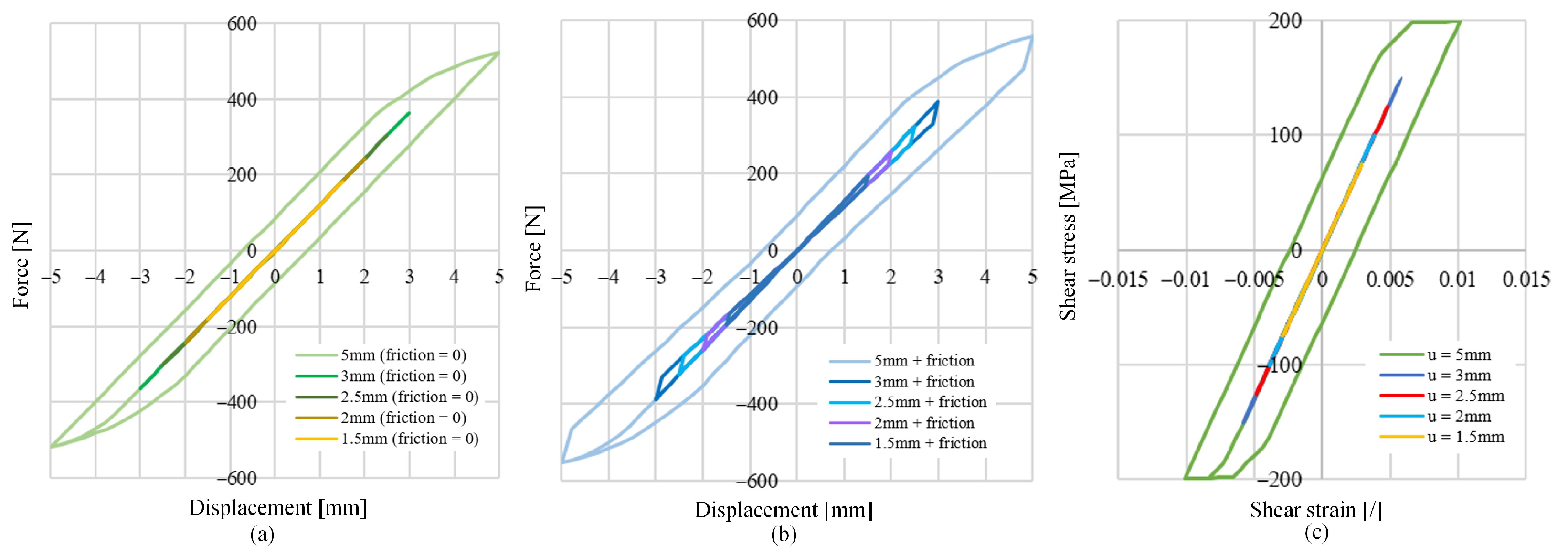
In the simulation, the force on the test rig was measured between the carriers 1 and 2 (Figure 5). To calculate the reaction force, all the reaction forces at the nodes between the carrier surfaces were summed. The results of the numerical simulation for the displacements of 1.5, 2.0, 2.5, 3.0, and 5.0 mm are presented in Figure 8a,b. For displacements between mm and mm, the force on the test rig changed linearly when there was no friction in the system. However, when friction was considered in the sliding contacts, the force on the test rig increased or decreased due to the friction force. When the U profile moved in positive direction of displacement u, the force on the test rig was enlarged for the friction force in the mechanism. When transitioning from the maximum displacement value to the initial position, the force value was reduced by twice the value of the friction force. After crossing the initial position, the force on the test rig was still reduced by the friction force value. In the extreme position, when the U profile started returning from the furthest point of negative displacement towards the initial position, the force on the test rig was instantly increased by twice the value of the friction force. However, the signal in the diagram indicates the elastic behaviour of the specimen, which can be obtained by comparison with the frictionless response (Figure 8a,b). On the contrary, when the specimen was loaded at a displacement level of mm, the force response became nonlinear, even in the absence of friction between the components of the cyclic torsional adapter. A hysteresis loop was thus formed, thereby suggesting the transition of the specimen into the elastoplastic region of loading. Here, the system losses due to friction were evaluated as the difference between the maximal absolute force values at reversal points when friction was assumed to the values when there was no friction considered in the contacts. It turns out that the force on the test rig was increased by 6% on average due to friction when the coefficient of friction in the sliding contacts was assumed to equal 0.2.
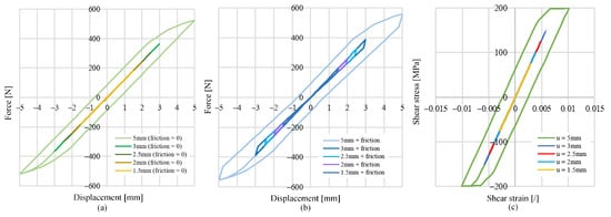
Figure 8.
Numerical simulation of (a) force displacement response at the test rig without consideration of friction, (b) force displacement response at the test rig with consideration of friction, and (c) stress–strain response of the specimen during constant amplitude loading with different displacements.
Figure 8c shows the shear stress –shear strain diagram result of the numerical simulation. The values were gained on the surface of the specimen in the middle of the measured gauge. For displacements between mm and mm, the response was a straight line. This indicates that the specimen was within the elastic range throughout the loading process at these loading levels. At the displacement of mm however, the specimen entered the elastoplastic region of the material, which resulted in a hysteresis loop. Importantly, the shear stress is presented in Figure 8c from the numerical stress results on the surface of the specimen. Since this position did not include the transfer of the loading over the cyclic torsional adapter, the same stress result was obtained regardless of the simulated friction in the mechanism. To observe the effect of friction, the value of the shear stress was extracted from the simulated force on the test rig (Figure 8a,b). These values are given below in Section 3.4.
3.3. Experimental Results
Nine specimens were tested experimentally. With the first group of specimens, LCF tests at displacements and mm were conducted. Strain gauges were attached to four specimens in order to establish the transfer function between the displacement of the test rig and the strain of the specimen. Three specimens served for the additional results of the durability curve. They were tested until failure at displacement levels of and mm. The remaining two specimens were used for the incremental step test (IST), which was performed to gain the stabilised cyclic shear stress–strain curve of the material. They were also equipped with strain gauges. The shear strain at reversal points for the three LCF specimens without strain gauges was then determined from the IST results, which are presented in detail in Section 3.4. The number of cycles to failure and the average values of the shear strain amplitudes are summarised in Table 6.
Table 6.
Experimental LCF test results for aluminium alloy Al6061. The specimens equipped with strain gauges are marked with an *.
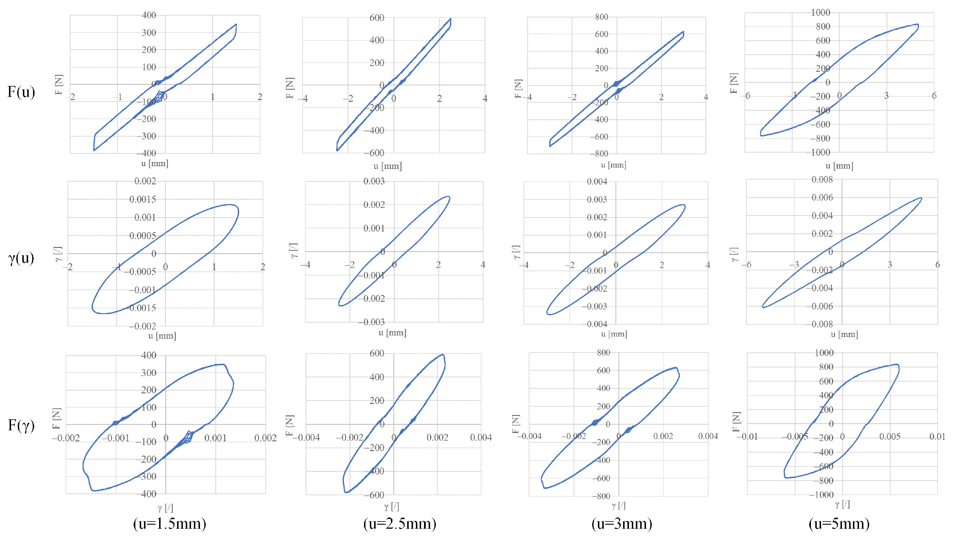
The force measurements on the test rig F, the displacements u, and shear strains can be compared for the four specimens equipped with strain gauges. The results are shown in Figure 9. The diagram shows the mutual dependence between the force F, displacement u, and shear strain .
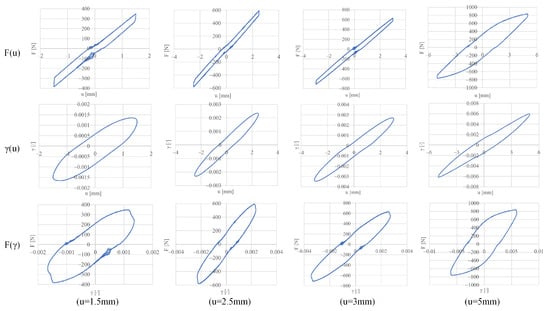
Figure 9.
F, , and F( relations for tested load levels.
Looking at the F and F diagrams, linear dependence can be noticed for small values of u and , whereas a nonlinear response can be observed for mm. The nonlinearity in this case is a consequence of the elastoplastic response of the specimen. On the contrary, the response is linear, as the displacement of the test rig and the strain on the specimen are directly connected through the mechanism of the cyclic torsional adapter. Nevertheless, some oscillations of the force signal in both the vertical and the horizontal directions of F and F during the crossing of the neutral position can be seen. This effect is a consequence of the displacement or tilting of the vertical bars away from their equilibrium position due to the slight clearance in the contacts of the mechanism. Moreover, when reaching the extreme displacement limit u, a sudden drop in the force signal can be observed most clearly in the F response. This effect is attributed to the frictional force in the mechanism. Regardless of the displacement amplitude, the values of the force drop when crossing the upper extreme limit and force jump when crossing the lower extreme limit were approximately 60 N. To reduce or eliminate this effect, the reduction of friction in the mechanism would be mandatory.
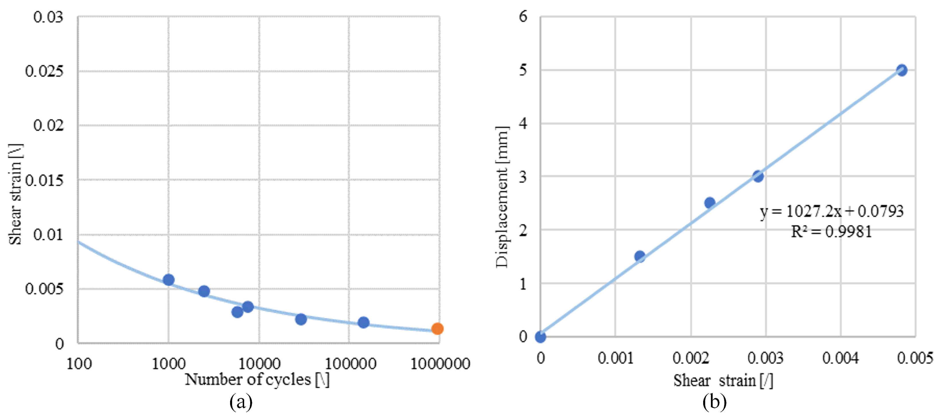
The durability curve can be created from the shear strain results. It is presented in Figure 10a. The Manson–Coffin–Morrow-type curve,
was determined based on the measurements at the amplitude levels of mm. The parameters are given in Table 7. A total of 510,000 cycles to failure at a displacement level of mm were then predicted. The prediction was compared to the experimental result, where 941,766 cycles at a 1.5 mm displacement amplitude were reached. The point is plotted with orange colour in the diagram in Figure 10a. It can be seen that in the logarithmic scale, this point and the approximation curve match substantially.
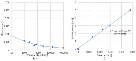
Figure 10.
Durability curve for aluminium alloy Al6061 (a) and geometric dependence between displacement of the test rig and shear strain (b). The curves were determined from blue points. The orange point represents the experimental result at displacement level of mm (shear strain level of ). The orange point and the approximation curve match substantially.
Table 7.
Manson–Coffin–Morrow parameters for durability curve of aluminium alloy Al6061.
If a large number of specimens is to be tested, the process of attaching strain gauges to each specimen can be too time-consuming and somewhat superfluous. A displacement–shear strain diagram can thus aid the establishment of either the cyclic stress–strain curve or the durability curve for the reversal points (Figure 10b). Namely, the geometric link between the displacement of the test rig and shear strain on the specimens provides a unique and definite result. To determine the shear strain, strain gauges are no longer needed; only the information regarding the displacement on the test rig must be recorded during the test. Then, based on the displacement–shear strain diagram, the corresponding shear strain for the specimens is determined. Even in the case of a different material of the specimens, a new calibration is not needed. Admittedly, the stress–strain curve between the reversal points might not be accurate due to the influence of the friction in the recorded force signal, but the state in the reversal points is correct.
3.4. Correlations
3.4.1. Incremental Step Tests
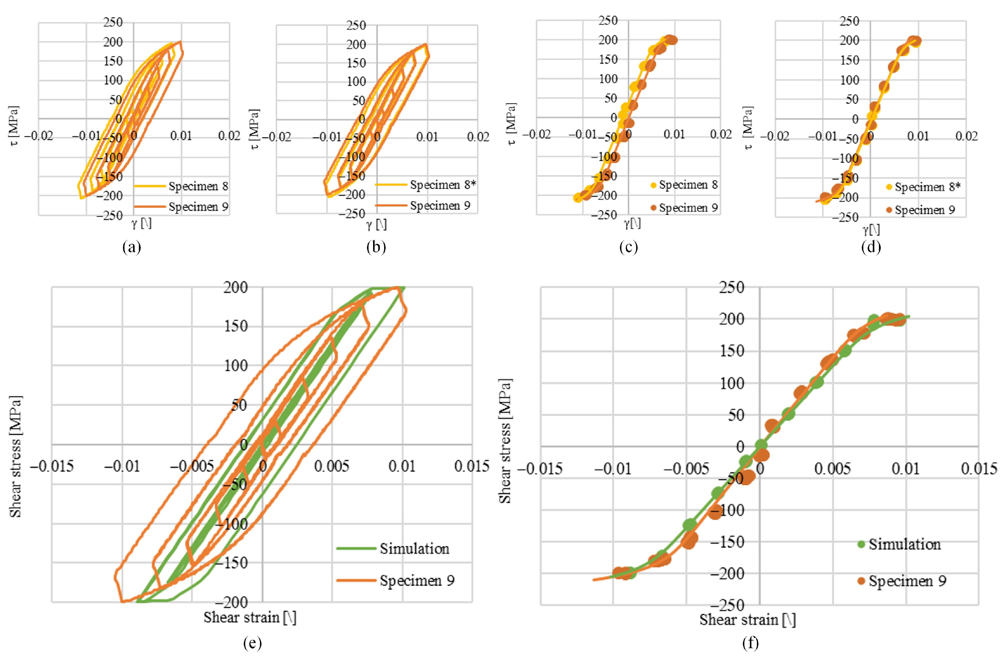
Numerical and experimental ISTs for a nominal displacement amplitude of mm were performed. Two physical specimens, equipped with strain gauges, were used for the IST. The course of the signal for the ISTs is given in Figure 5e. The recorded experimental results for the stabilised response of the material during the IST are presented in Figure 11a.
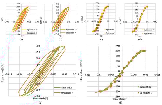
Figure 11.
Results of the incremental step test for nominal displacement amplitude value of 5 mm: recorded (a) – response, (b) shifted – response for specimen 8 (marked with *), (c) recorded reversal points, (d) shifted reversal points for specimen 8 (marked with *), (e) comparison of stress–strain response with simulation results, and (f) comparison of reversal points with simulation results.
As the signal for specimen 8 drifted during the test, it was afterwards corrected by a +0.0015 shift (Figure 11b). Moreover, stabilised reversal points were extracted for the determination of the cyclic stress–strain curve. The recorded values are given in Figure 11c, and the shifted values are given in Figure 11d. It can be noticed that an appreciable repeatability of the results was achieved. Evidently, the numerical and experimental hysteresis loops show the same phenomenon (Figure 11e). But since the experimental hysteresis loops were wider compared to the simulated loops, the discrepancies must be attributed to the friction circumstances in the torsional adapter. Specifically, the lateral friction between the components, which was not taken into account in the simulation, could be the cause for the mismatch of the signals. Nevertheless, the numerical and experimental results in the reversal points completely match (Figure 11f). It has thus been confirmed again that the reversal points obtained from the experimental results are correct, whereas the recorded paths between the reversal points can rather serve for orientation purposes.
A stabilised cyclic stress–strain curve was determined from the recorded signals using the Ramberg–Osgood equation:
The parameters used in the Ramberg–Osgood equation are presented in Table 8.
Table 8.
Parameters for Ramberg–Osgood type stabilised cyclic stress–strain curve of aluminium alloy Al6061 determined using the cyclic torsional adapter.
3.4.2. Stress–Strain Relations
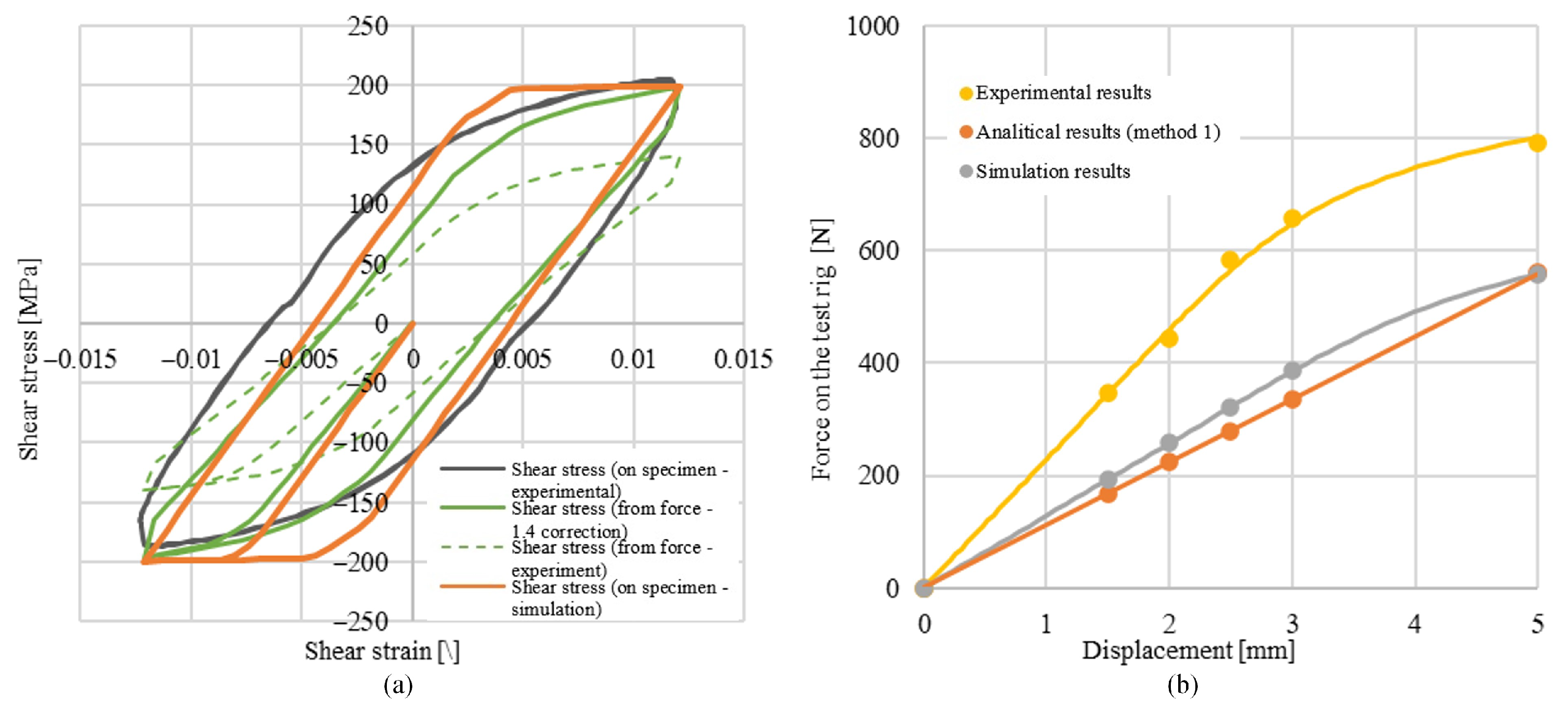
The shear stress and shear strain results of the experiment and simulation are compared for a displacement level of mm in Figure 12a. A hysteresis loop was formed at this excitation level. The experimental hysteresis loop appeared to be the widest, which was seemingly due to the friction in the hinge contacts of the torsional adapter and also between the components in the lateral direction. Moreover, two simulated curves were established. The orange curve represents the response as simulated directly on the surface of the specimen. The influence of friction is not visible in this curve. However, the green curve stands for the shear stress simulated from the force on the test rig. This value was corrected by a factor of 1.4 to consider the overall experimental friction losses in the cyclic torsional adapter. In the reversal points, a characteristic change of the stress value was observed due to the friction in the mechanism. A comparison between the experimental and the simulated results provides a good agreement of the signals.
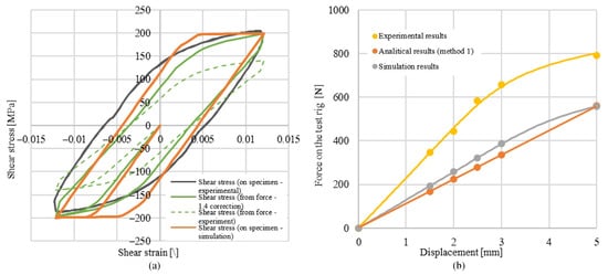
Figure 12.
Comparison of (a) experimental and simulated values of the stress–strain response and (b) experimental, analytical, and simulated reversal points.
3.4.3. Force on the Test Rig
The force and displacement on the test rig can be compared between the analytical, numerical, and experimental observations (Figure 12b). The simulation results and the analytical results with the consideration of friction model 1 differed by 15% for displacements of up to 3 mm. For the load level of mm, the results were the same. Importantly however, the force on the test rig in the analytical model rose proportionally with increasing displacement, whereas both the simulation and the experimental results indicate an exponential growth of the force as a function of the displacement. This discrepancy arises due to the elastoplastic behaviour of the specimen, which was not considered in the analytical model. On average, the experimental force values on the test rig were 50% higher than the values in the simulation and analytical model for displacements up to 3 mm. At the displacement level of 5 mm, the force on the test rig was around 30% higher than the analytically calculated value. The higher values of the experimentally measured force on the test rig can be attributed to the lateral friction between the components of the torsional adapter, which was not taken into account in the current analytical and numerical models.
Both experimental and simulation force–displacement results can also be approximated using a Ramberg–Osgood-type curve:
The parameters are presented in Table 9.
Table 9.
Ramberg–Osgood parameters for the relation between the force on the test rig and the displacement.
The comparison of the parameters confirms the similarity of the experimental and the numerical curve. Namely, the shape of the curve is given by the parameter , whilst the height of the initial part of the curve is set by the parameter . It can be noticed that the same optimal parameter was calculated to approximate the experimental and simulation results. Moreover, the presence of the lateral friction in the experimental results is indicated by a higher value of the parameter .
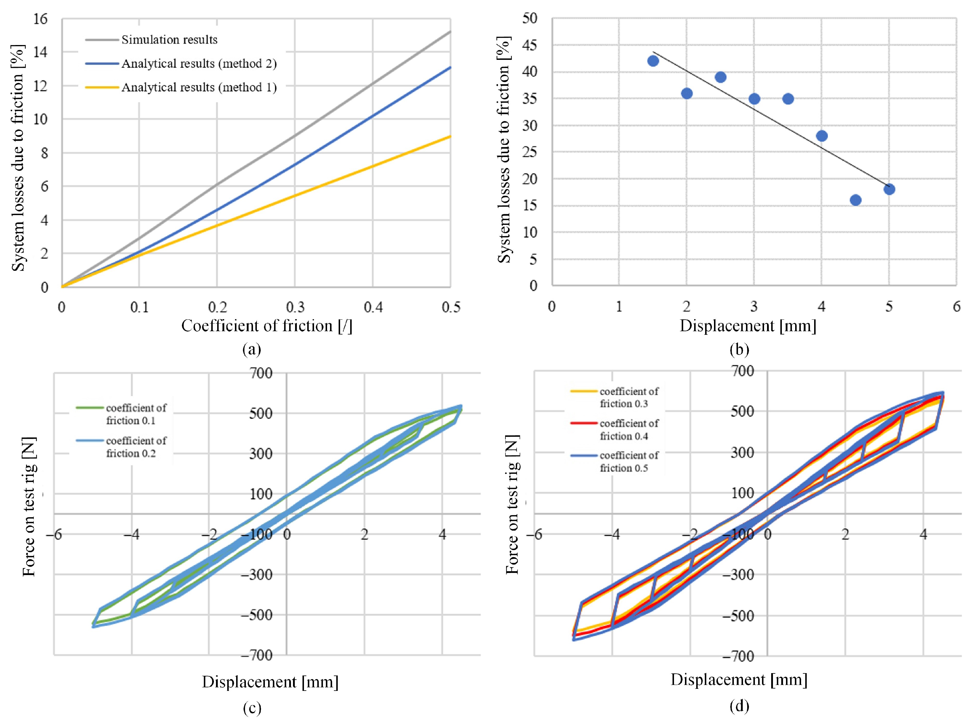
3.4.4. Sensitivity Analysis of the Torsional Adapter
If the magnitude of the force on the test rig is tracked in the numerical model, the proportion of system losses due to friction can be analysed. To better understand the influence of the friction coefficient on the simulation results, a sensitivity analysis was performed for the IST by varying the values of the friction coefficient in the contacts of the mechanism from to . The results are collected in the form of hysteresis loops in Figure 13c,d. The magnitude of the force predicted on the test rig at different coefficients of friction was compared to the results of the numerical simulation performed with frictionless conditions in the system and ideal sliding contacts. The difference in forces then represents the system losses due to friction. If these values are compared to the system losses of the analytical model for various friction coefficients, the result in Figure 13a is obtained. It can be noticed that the numerical results lie close to the results of the analytical model considering method 2 for the friction. Specifically, the analytically calculated losses considering method 1 reached up to 10%. The analytically calculated losses considering method 2 followed with around 13% of losses. The highest system loss prediction was obtained by the numerical model. According to this prediction, the system losses would reach up to 15% at the friction coefficient of 0.5.
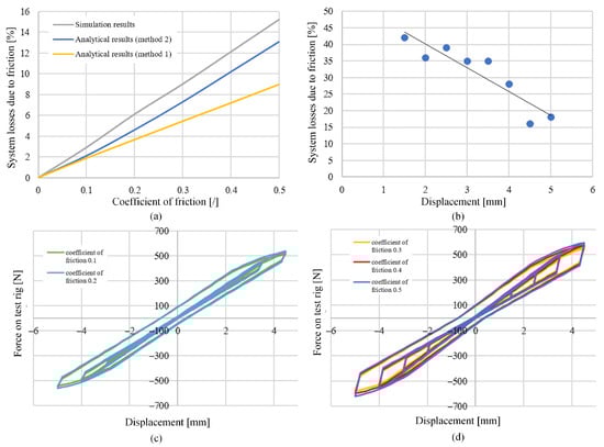
Figure 13.
Results of sensitivity analysis regarding the coefficient of friction: (a) comparison of numerical and analytical models, (b) experimental system losses, (c) results of numerical simulation for the values of friction coefficient 0.1 and 0.2, and (d) results of numerical simulation for the values of friction coefficient 0.3, 0.4, and 0.5.
The experimental system losses were determined as follows. The extreme values of force at reversal points of the IST (for specimen 9) were collected. Next, the system losses were calculated against the expected analytical solution using method 1 to consider friction for the same values of displacement. The course of system losses as a function of displacement u is presented in Figure 13b. A negative trend of the system losses was observed, i.e., the higher the displacement u on the test rig, the smaller force proportion needed to overcome the friction force. Specifically, at smaller displacements ( mm), the losses could reach over 40%. With increasing displacements ( and 5 mm), the losses fell below 20%.
If the system losses between the analytical, numerical, and experimental consideration are to be equalised, a coefficient of friction in the sliding contacts for the analytical and numerical model between and is needed. This result therefore clearly shows that the lateral friction between the components is considerable and would have to be considered in the numerical and analytical models in order to create realistic comparisons. With consideration of lateral friction in simulations, realistic values of the friction coefficient in the sliding contacts could also be applied. Future improvements of the models will therefore include the lateral friction between the components of the torsional adapter. Another option for the improvement of the torsional adapter is in the direction of omission of the sliding contacts in the mechanism.
4. Conclusions
Torsional adapters for tensile–compression test machines are not widespread. Little information about such designs is available. The evaluation of friction is mostly the biggest challenge.
The cyclic torsional adapter presented here enables the determination of both the cyclic shear stress–strain curve and the durability curves.
Analytical and numerical models were set to analyse the behaviour of the adapter during operation. The analytical model includes the kinematics of the mechanism and two methods to evaluate friction losses. The numerical model was set using the implicit finite element method and enables consideration of the elastoplastic material properties of the specimen and friction losses in the contacts of the mechanism. For the aluminium alloy Al6061 specimens, up to 10% losses were predicted by analytical and numerical simulations prior to the experiments.
Experimentally, low-cycle fatigue tests and incremental step tests were performed using the cyclic torsional adapter. The experimental setup enabled data acquisition from the displacement and force measurements at the test rig and strain from the strain gauges mounted onto the specimens. Additionally, the recorded number of cycles to failure allowed for the determination of the torsional durability curve of the tested material. The experimental system losses due to friction varied between 20 and 40%, depending on the displacement u.
In a simulated incremental step test, the numerically determined reversal points of the hysteresis loops coincided with experimental values. Nevertheless, to improve the prediction of the analytical and numerical models, the lateral friction between the components should be taken into account in future research.
Author Contributions
Conceptualization, D.Š. and J.K.; methodology, D.Š. and J.K.; software, K.G., A.Š. and D.Š.; validation, K.G., A.Š., J.K. and D.Š.; formal analysis, K.G. and D.Š.; investigation, K.G., A.Š. and D.Š.; resources, J.K.; data curation, K.G., A.Š. and D.Š.; writing—original draft preparation, K.G. and D.Š.; writing—review and editing, K.G., A.Š., J.K. and D.Š.; visualization, K.G. and D.Š.; supervision, D.Š. and J.K.; project administration, D.Š.; funding acquisition, J.K. All authors have read and agreed to the published version of the manuscript.
Funding
The authors acknowledge financial support from the Slovenian Research Agency (research core funding No. P2-0182 entitled Development Evaluation).
Data Availability Statement
Data are contained within the article.
Acknowledgments
The authors appreciate the efforts of the students who took the course Effectiveness of Products in the academic year 2021/2022 and Naëvan Avinin regarding the initial design of the torsional adapter.
Conflicts of Interest
The authors declare no conflicts of interest. The funders had no role in the design of the study; in the collection, analyses, or interpretation of data; in the writing of the manuscript, or in the decision to publish the results.
References
- Huang, L.; Lu, Y.; Shi, C. Unified Calculation Method for Symmetrically Reinforced Concrete Section Subjected to Combined Loading. ACI Struct. J. 2013, 110, 127–136. [Google Scholar]
- Traphöner, H.; Clausmeyer, T.; Tekkaya, A.E. Material characterization for plane and curved sheets using the in-plane torsion test—An overview. J. Mater. Process. Technol. 2018, 257, 278–287. [Google Scholar] [CrossRef]
- Liu, W.; Lian, J.; Münstermann, S. Damage mechanism analysis of a high-strength dual-phase steel sheet with optimized fracture samples for various stress states and loading rates. Eng. Fail. Anal. 2019, 106, 104138. [Google Scholar] [CrossRef]
- Feng, Q.; Zhu, Z.; Tong, Q.; Yu, Y.; Zheng, W. Dynamic responses and fatigue assessment of OSD in heavy-haul railway bridges. J. Constr. Steel Res. 2023, 204, 107873. [Google Scholar] [CrossRef]
- Saadouki, B.; Sapanathan, T.; Pelca, P.; Elghorba, M.; Rachik, M. Failure analysis and damage modeling of precipitate strengthened Cu–Ni–Si alloy under fatigue loading. Procedia Struct. Integr. 2018, 9, 186–198. [Google Scholar] [CrossRef]
- Sun, H.; Guo, W.; Wang, L.; Rong, B. An analysis method of dynamic requirement change in product design. Comput. Ind. Eng. 2022, 171, 108477. [Google Scholar] [CrossRef]
- Li, C.; Zhou, J.; Ke, L.; Yu, S.; Li, H. Failure mechanisms and loading capacity prediction for rectangular UHPC beams under pure torsion. Eng. Struct. 2022, 264, 114426. [Google Scholar] [CrossRef]
- Roesler, C.R.M.; Salmoria, G.V.; Moré, A.D.O.; Vassoler, J.M.; Fancello, E.A. Torsion test method for mechanical characterization of PLDLA 70/30 ACL interference screws. Polym. Test. 2014, 34, 34–41. [Google Scholar] [CrossRef]
- Ju, H.; Han, S.J.; Kim, K.S. Analytical model for torsional behavior of RC members combined with bending, shear, and axial loads. J. Build. Eng. 2020, 32, 101730. [Google Scholar] [CrossRef]
- Huang, Y.; Yang, J.; Feng, R.; Chen, H. Resistance of cold-formed sorbite stainless steel circular tubes under uniaxial compression. Thin-Walled Struct. 2022, 179, 109739. [Google Scholar] [CrossRef]
- Hao, P.; Spronk, S.; Van Paepegem, W.; Gilabert, F. Hydraulic-based testing and material modelling to investigate uniaxial compression of thermoset and thermoplastic polymers in quasistatic-to-dynamic regime. Mater. Des. 2022, 224, 111367. [Google Scholar] [CrossRef]
- Zhang, Y.; Fang, C.; Wang, W.; Hou, H. Cyclic plasticity and ULCF behavior of steel butt-joints considering different welding methods. Int. J. Fatigue 2023, 173, 107684. [Google Scholar] [CrossRef]
- Dong, H.; Li, X.; Li, Y.; Wang, H.; Peng, X.; Zhang, S.; Meng, B.; Yang, Y.; Li, D.; Balan, T. An experimental and modelling study of cyclic tension-compression behavior of AA7075-T6 under electrically-assisted condition. J. Mater. Process. Technol. 2022, 307, 117661. [Google Scholar] [CrossRef]
- Yang, B.; Jiang, Q.; Feng, X.; Xin, J.; Xu, D. Shear testing on rock tunnel models under constant normal stress conditions. J. Rock Mech. Geotech. Eng. 2022, 14, 1722–1736. [Google Scholar] [CrossRef]
- Turvey, G.J. Torsion tests on pultruded GRP sheet. Compos. Sci. Technol. 1998, 58, 1343–1351. [Google Scholar] [CrossRef]
- Wu, H.C.; Xu, Z.; Wang, P.T. Torsion test of aluminum in the large strain range. Int. J. Plast. 1997, 13, 873–892. [Google Scholar] [CrossRef]
- Małecka, J.; Łagoda, T. Fatigue and fractures of RG7 bronze after cyclic torsion and bending. Int. J. Fatigue 2023, 168, 107475. [Google Scholar] [CrossRef]
- Bressan, J.D.; Unfer, R.K. Construction and validation tests of a torsion test machine. J. Mater. Process. Technol. 2006, 179, 23–29. [Google Scholar] [CrossRef]
- Timercan, A.; Terriault, P.; Brailovski, V. Axial tension/compression and torsional loading of diamond and gyroid lattice structures for biomedical implants: Simulation and experiment. Mater. Des. 2023, 225, 111585. [Google Scholar] [CrossRef]
- Fu, S.; Wang, L.; Chen, G.; Yu, D.; Chen, X. A tension-torsional fatigue testing apparatus for micro-scale components. Rev. Sci. Instruments 2016, 87, 015111. [Google Scholar] [CrossRef]
- Shen, Y.; Fu, S.; Shi, S.; Chen, X. Torsional fatigue with axial constant stress of oligo-crystalline 316L stainless steel thin wire. Fatigue Fract. Eng. Mater. Struct. 2018, 41, 1929–1937. [Google Scholar] [CrossRef]
- Petit, J.; Jiang, Z.; Polit, O.; Palin-Luc, T. Optimisation of an ultrasonic torsion fatigue system for high strength materials. Int. J. Fatigue 2021, 151, 106395. [Google Scholar] [CrossRef]
- Ogawa, F.; Shimizu, Y.; Bressan, S.; Morishita, T.; Itoh, T. Bending and Torsion Fatigue-Testing Machine Developed for Multiaxial Non-Proportional Loading. Metals 2019, 9, 1115. [Google Scholar] [CrossRef]
- Achtelik, H.; Kurek, M.; Kurek, A.; Kluger, K.; Pawliczek, R.; Łagoda, T. Non-standard fatigue stands for material testing under bending and torsion loadings. AIP Conf. Proc. 2018, 2029, 020001. [Google Scholar]
- Goanta, V. Device for Torsional Fatigue Strength Assessment Adapted for Pulsating Testing Machines. Sensors 2022, 22, 2667. [Google Scholar] [CrossRef]
- Středulová, M.; Lisztwan, D.; Eliáš, J. Friction effects in uniaxial compression of concrete cylinders. Procedia Struc. Integ. 2022, 42, 1537–1544. [Google Scholar] [CrossRef]
- Maleki, M.; Ahmadian, H.; Rajabi, M. A modified Bouc-Wen model to simulate asymmetric hysteresis loop and stochastic model updating in frictional contacts. Int. J. Solids Struct. 2023, 269, 112212. [Google Scholar] [CrossRef]
- Farfan-Cabrera, L.I.; Pérez-González, J.; Iniestra-Galindo, M.G.; Marín-Santibáñez, B.M. Production and tribological evaluation of polypropylene nanocomposites with reduced graphene oxide (rGO) for using in water-lubricated bearings. Wear 2021, 477, 203860. [Google Scholar] [CrossRef]
- You, H.; Zhu, C.; Li, W. Contact Analysis on Large Negative Clearance Four-point Contact Ball Bearing. Procedia Eng. 2012, 37, 174–178. [Google Scholar]
- Tan, H.; Hu, Y.; Li, L. Effect of friction on the dynamic analysis of slider-crank mechanism with clearance joint. Int. J. Non-Linear Mech. 2019, 115, 20–40. [Google Scholar] [CrossRef]
- Benavides, J.E.H.; Corredor, D.E.E.; Moreno, R.J.; Hernandez, R.D.; Alfonso, D.H. Analysis od Friction Systems on Shafts for Engineering Applications. Int. J. Appl. Eng. Res. 2018, 13, 8871–8881. [Google Scholar]
- Šeruga, D.; Nagode, M. Comparative analysis of optimisation methods for linking material parameters of exponential and power models: An application to cyclic stress–strain curves of ferritic stainless steel. J. Mater. Des. Appl. 2019, 233, 1802–1813. [Google Scholar] [CrossRef]
- Armstrong, P.J.; Frederick, C.O. A Mathematical Representation of the Multiaxial Bauschinger Effect; Berkeley Nuclear Laboratories: Berkeley, CA, USA, 1966; Volume 731. [Google Scholar]
- Chaboche, J.L. A review of some plasticity and viscoplasticity constitutive theories. Int. J. Plast. 2008, 24, 1642–1693. [Google Scholar] [CrossRef]
- Carazo, F.D.; Alés, J.J.P.; Signorelli, J.; Celentano, J.D.; Guevara, C.M.; Lucci, R. Analysis of Strain Inhomogeneity in Extruded Al 6061-T6 Processed by ECAE. Metals 2022, 12, 299. [Google Scholar] [CrossRef]
- Hoffmann, K. An Introduction to Measurements using Strain Gages; Hottinger Baldwin Messtechnik GmbH: Darmstadt, Germany, 1987. [Google Scholar]
- Wittel, H.; Muhs, D.; Jannasch, D.; Voßiek, J. Roloff/Matek Maschinenelemente; Springer Fachmedien: Wiesbaden, Germany, 2013. [Google Scholar]
Disclaimer/Publisher’s Note: The statements, opinions and data contained in all publications are solely those of the individual author(s) and contributor(s) and not of MDPI and/or the editor(s). MDPI and/or the editor(s) disclaim responsibility for any injury to people or property resulting from any ideas, methods, instructions or products referred to in the content. |
© 2024 by the authors. Licensee MDPI, Basel, Switzerland. This article is an open access article distributed under the terms and conditions of the Creative Commons Attribution (CC BY) license (https://creativecommons.org/licenses/by/4.0/).