Adopting New Machine Learning Approaches on Cox’s Partial Likelihood Parameter Estimation for Predictive Maintenance Decisions

Abstract

The Proportional Hazards Model (PHM) under a Condition-Based Maintenance (CBM) policy is used by asset-intensive industries to predict failure rate, reliability function, and maintenance decisions based on vital covariates data. Cox’s partial likelihood optimization is a method to assess the weight of time and conditions into the hazard rate; however, parameter estimation with diverse covariates problem could have multiple and feasible solutions. Therefore, the boundary assessment and the initial value strategy are critical matters to consider. This paper analyzes innovative non/semi-parametric approaches to address this problem. Specifically, we incorporate IPCRidge for defining boundaries and use Gradient Boosting and Random Forest for estimating seed values for covariates weighting. When applied to a real case study, the integration of data scaling streamlines the handling of condition data with diverse orders of magnitude and units. This enhancement simplifies the modeling process and ensures a more comprehensive and accurate underlying data analysis. Finally, the proposed method shows an innovative path for assessing condition weights and Weibull parameters with data-driven approaches and advanced algorithms, increasing the robustness of non-convex log-likelihood optimization, and strengthening the PHM model with multiple covariates by easing its interpretation for predictive maintenance purposes.

1. Introduction

Physical Asset Management (PAM) is a critical aspect of modern industrial operations, as it involves the maintenance and optimization of system equipment to ensure their reliability, availability, and safety. As part of PAM, the Proportional Hazards Model (PHM) focuses on predicting the failure risk of assets based on their current condition and historical data. With PHM, it is possible to estimate conditional reliability functions and remaining useful life (RUL). Accurate RUL prediction can help reduce downtime, maintenance costs, and safety risks and improve the overall efficiency of industrial operations.

Predictive maintenance stands out as particularly interesting within the field of maintenance policies. It aims to determine the optimal intervention time of equipment, thereby minimizing the likelihood of failure through diverse techniques. A noteworthy approach within predictive maintenance is Condition-Based Maintenance (CBM), which operates as a prognostic policy by estimating equipment failure rates and reliability using present and anticipated conditions. Hence, the methodology involves continuous monitoring of those vital signs, in which PHM assigns weights to individual conditions, enabling the calculation of the equipment’s failure risk at any given moment.

In recent years, there has been a growing interest in using data-driven approaches and advanced algorithms to improve the accuracy of PHM modeling. In the same way, estimating parameters in PHM models with multiple covariates is challenging due to the log-likelihood function non-convex nature and the high dimensionality of the parameter space. In order to address this challenge, this work proposes a non-conventional methodology that combines non/semi-parametric approaches, such as Random Forest and Genetic Algorithm, to estimate the covariate weights and Weibull parameters in PHM models with multiple vital signs.

Cox’s partial likelihood optimization is usually employed to evaluate the impact of time and conditions on the hazard rate. However, when dealing with parameter estimation involving diverse covariates, the problem may have multiple feasible solutions. Consequently, assessing boundaries and carefully adopting an effective initial value strategy is imperative. Therefore, this paper explores innovative non/semi-parametric approaches to address these issues. Specifically, we integrate IPCRidge to define boundaries and leverage Gradient Boosting and Random Forest to estimate initial covariate weighting values. The proposed methodology is evaluated in a real-world case study in an asset-intensive firm to demonstrate the integration of condition data scaling with diverse orders of magnitude and units.

The rest of this paper is organized as follows. Section 2 provides a literature review of the existing approaches to PHM and parameter estimation. Section 3 describes the proposed methodology in detail, including the data-driven approaches and advanced algorithms used. Section 4 presents the case study and discusses the results obtained. Finally, Section 5 concludes the paper and outlines the future research directions.

2. Literature Review

2.1. Physical Asset Management (PAM)

PAM has gained greater relevance in recent years among asset-intensive companies, given its ability to integrate with maintenance decisions, making the performance of operations more efficient and safer. This approach has been implemented using Asset Management Systems (AMS), which reduces risk and asset life cycle costs [1,2,3].

Given industries’ recent and cross-cutting technological development, advanced tools can be adopted to improve asset and process management, such as predictive maintenance and data-driven techniques [4,5,6]. CBM, as a predictive policy, allows for making maintenance decisions based on information collected through the monitoring of asset conditions, such as temperature or pressure, in order to predict asset failures; this method improves asset health management and reduces the life cycle cost of assets [3,7]. As stated in [2], CBM is a key factor of PAM and very important for developing an ASM.

2.2. Proportional Hazards Model (PHM)

As a statistical procedure, PHM estimates equipment failure risk based on condition-monitoring information [8,9]. The way to describe Cox’s PHM is the baseline hazard function that normally is used by assuming Weibull distribution due to its flexibility and closed-form risk and reliability function [10,11], but others like the Gamma distribution could be used as well [12]. Similarly, ref. [13] develops a method for calculating reliability and remaining useful life (RUL) based on current conditions and presents a case study with one covariate. In a step of the method, data must be discretized in several states, each one with a representative reliability function. These functions are depicted graphically, showing the differences in their wear-out rates. Another relevant approach is presented in [9] with a method to optimize CBM for the decision-making process of asset interventions with multiple covariates, transition probability matrices, PHM, and the costs associated with corrective and preventive interventions. This method is expressed and condensed as software for industry applications.

The paragraph above introduces the relevant matter of this paper, the parameter estimation for Weibull distribution with multiple covariates, considering them in the hazard rate and conditional reliability function. There are many approaches to this particular matter, and some of the most relevant are discussed as follows. Ref. [8] shows a way to obtain the covariate coefficients/weights with Maximum Likelihood Estimation (MLE). Although the distribution parameters are not explicitly stated, Cox suggests assuming a two-parameter distribution such as Weibull or Exponential to model the baseline hazard rate and add these parameters inside MLE.

The two most widely used failure risk/survival analysis techniques are Cox’s PHM and Accelerated Failure Time Model (AFTM) [14]. Due to their flexibility and efficiency, one of the main differences between the two is that Cox’s PHM is a semi-parametric method where no assumptions are imposed on the baseline hazard function [15]. Ref. [16] proposes a method that uses MLE to obtain Weibull distribution parameters (shape and scale) and weight/importance of the covariates; specifically, the authors analyze PHM as an AFTM so they can estimate shape, scale, and covariate weights parameters with just one likelihood function. Nevertheless, the main issue is the non-linear nature of these MLE functions, so analytical solutions are not simple to obtain [17]. Ref. [18] shows a non-analytical way to solve it; the authors use a defined baseline hazard rate, specifically the Weibull hazard rate, so the model is called Weibull-PHM, or the Weibull regression model. They maximize the associate likelihood function using the Broyden–Fletcher–Goldfarb–Shanno (BFGS) quasi-Newton method [19], so the Weibull parameters and six covariate weights are estimated. One limitation of the proposed method is that BFGS is sensitive to initial conditions. If the initial value is far from the global minimum, BFGS may fail to converge or converge to a local minimum. A second limitation is that BFGS does not guarantee global convergence, so for non-convex objective functions such as the Weibull PHM’s MLE function, BFGS may fail [20,21]. In addition, the Weibull PHM’s MLE function needs reasonable starting values, according to [22]. Therefore, the boundaries and the initial value are important matters to consider for the problem-solving strategy.

2.3. Data Driven PHM

The requirement for data-driven methods is emphasized in [23] as essential for implementing and deploying more sophisticated PHM-CBM systems. Recently, some studies have tried to incorporate non-parametric approaches to obtain Weibull PHM parameters. For instance, a data-driven method that uses meta-heuristic rules to obtain relationships between internal features of available data and its insights is presented in [24]. Data-driven models have been widely used in several fields with successful results [3,17,24,25,26].

One of the main pillars of recent technological development is Artificial Intelligence (AI) and Machine Learning (ML) [27], which could be described as the use of algorithms that learn from experiences as a human being would do [3,28]. Furthermore, experience is related to data, i.e., by showing them what to search for (supervised learning) or not (unsupervised learning) or by punishing/rewarding them during learning (reinforcement learning) [3,29]. Work [30] applies Gradient Boosting techniques (supervised learning) to evaluate the quality of the inputs for an optimization problem, which is solved using the Artificial Bee Colony (ABC) algorithm, an Evolutionary/Data Driven algorithm for optimization close to reinforcement learning family, such as Genetic Algorithm (GA) or Ant Colony Optimization (ACO). Hence, Gradient Boosting minimizes the potential of ABC being trapped in a local optimum and makes it possible to obtain a global optimum by identifying the most informative features. This study demonstrates that the feature selection using Gradient Boosting does not sacrifice model accuracy and outperforms the optimization results with different datasets. Other studies have used Random Forest to improve the Evolutionary algorithm performance [31,32], reaching conclusions similar to those of [30].

Evolutionary algorithms (EA) are characterized by simple parameters, broad applicability, generality, and ease of implementation, and they have found success across various domains [33]. GA is the most commonly used EA in the field of optimization problems [34] due to its implementation simplicity and capacity to converge into a solution that is close to the optimum in a prudent amount of time, but its accuracy relies on the selection of parameters [35], such as bounds and starting values. In [35], the GAs boosted with Machine Learning algorithms display better performance than just using GA, providing evidence that using Machine Learning techniques to adjust algorithm parameters is a promising approach. In fact, Machine Learning plays a pivotal role in navigating the search space, allowing algorithms to concentrate their computational efforts in the most promising directions for discovering better solutions.

Feature/covariate weighting is an important subject that MLE tries to solve in the present work. The authors of [15] present an approach using Multiple Kernel Learning (MKL), a supervised learning algorithm, for survival prediction models and the convex conjugate function for Cox’s PHM likelihood function. The study shows a robust performance in likelihood function estimation. Also, the MKL allows for the complexity of the boundaries to be avoided. Nevertheless, the study does not consider any assumption on the baseline hazard function, so the distribution parameters are not estimated in the MLE, and it uses a modified convex loss function for MLE. Study [36] proposes a Neural Network (NN) autoencoding (unsupervised learning) approach to estimate the robust features of a set. Then, Cox’s PHM and Long-Short Term Memory NN (LSTM) are used to predict the time between failures (TBF). So, the authors select the most important features for the prediction and use Cox’s PHM to obtain a reliability curve. They use MLE for the baseline hazard function and covariate weighting, but they do not specify any method to solve MLE. Ref. [26] uses reinforcement learning (Q-learning), Random Forest (RF) algorithm (supervised learning), and Markov Decision Process (MDP) for CBM optimization. The transition probability matrix is not used because the study relies completely on the meta-heuristics algorithms to obtain the reliability curves based on the Kaplan–Meier estimation method, which is non-parametric and asymptotically efficient [37,38], so the covariate weighting is made by using this method. Also, teh authors do not assume any distribution for wear-out; RF is used to predict this phenomenon. MDP incorporates the state space (defined by RF), action space (preventive and corrective interventions, `’do-nothing” policy, and multi-level preventive repair, `’as good as new” repair included), rewards (RUL), and punishments (maintenance cost). Q-learning is used to simulate a decision-maker agent that decides the action based on the “current” conditions of the data, costs, and expected RUL. A matter of concern for this study is the high computational cost related to the Q-learning method.

To enhance parameter estimation for the q-Weibull distribution, in [17], the Adaptive Hybrid Artificial Bee Colony (AHABC) algorithm is introduced. This innovative approach seamlessly integrates ABC’s global exploration capabilities with the local exploitation techniques of the Nelder–Mead simplex search, thereby improving ABC’s local search performance. Comparative analyses with alternative optimization methods, such as the Genetic Algorithm (GA) and Particle Swarm Optimization (PSO), reveal that the proposed AHABC algorithm surpasses them regarding convergence speed and accuracy. While the current study does not delve into the intricacies of covariate weighting, it echoes the showcased potential benefits of amalgamating various statistical and heuristic models. This scope aligns with the objective of the present work, which aims to explore and implement a similar integration of several models to take care of the boundaries and initial value strategy for Weibull PHM’s MLE.

3. Model Formulation

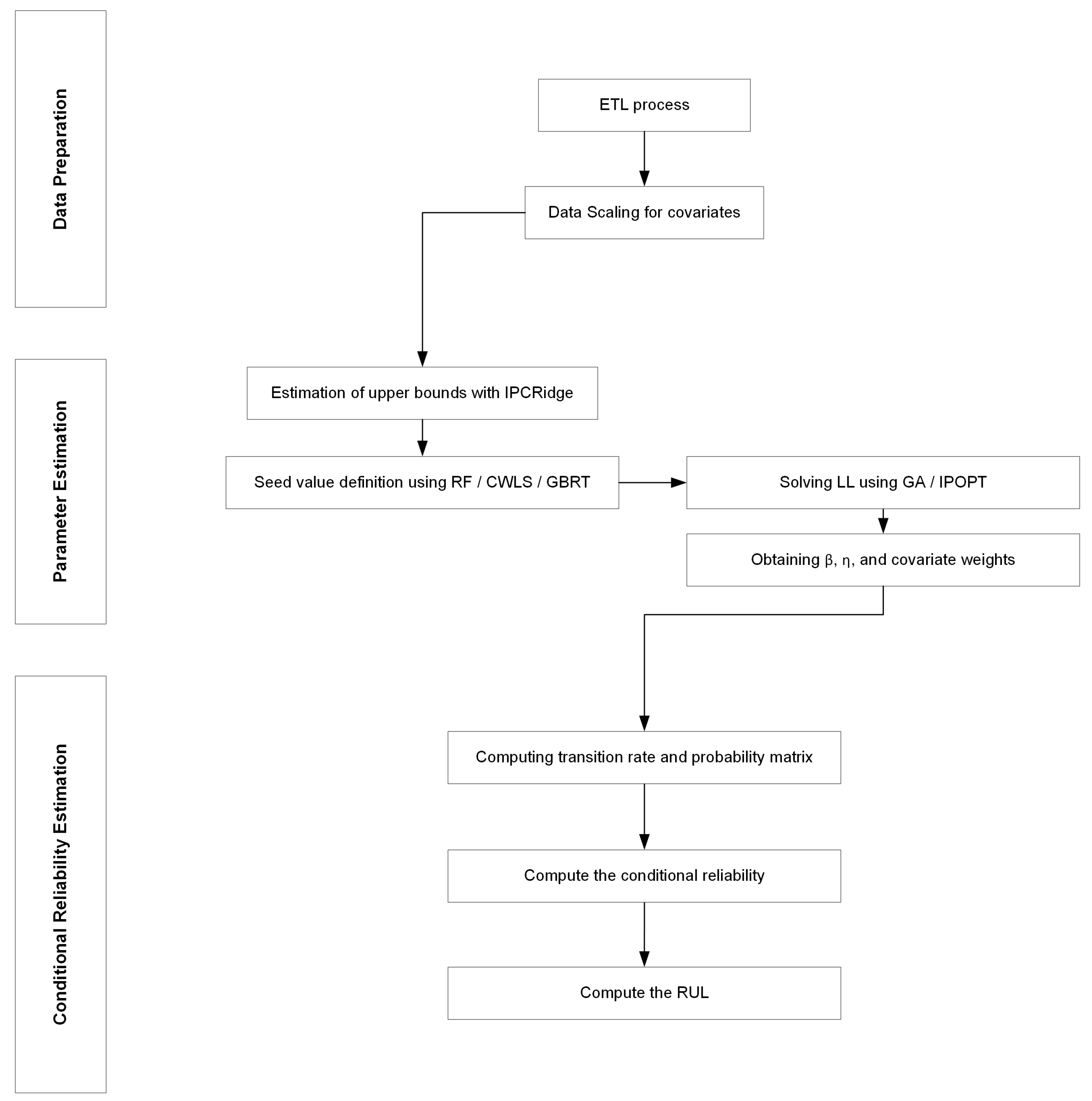
For the development of the present article, a flow chart of the analytical process was made, which can be seen in Figure 1.

3.1. Data Preparation and Data Scaling

First and foremost, data preparation is crucial to ensure the integrity of information before its utilization. This process involves thorough checks to eliminate null, missing, or duplicated data. Additionally, various tables are integrated through the ETL process (Extract, Transform, and Load) to consolidate all available information into a single dataset.

Simultaneously, a key aspect involves identifying and classifying maintenance types using a binary system. This binary system assigns values of 1 and 0 to preventive and corrective maintenance, respectively. The resulting table encapsulates only the pertinent data essential for model development. This includes an identifier for assets and their components (if applicable), the type of intervention represented in the binary system, the time intervals between interventions, and individual columns for each covariate.

Before working on covariate information, it is recommended to transform or standardize the data. An alternative is scaling this data to have the same order of magnitude and minimum and maximum values. This approach makes the analysis of the weights of each covariate easier, allowing for establishing their relative importance to one another. This study analyzes two transformation techniques: Min–Max scaling and a particular transformation representing a non-scaling alternative (NS). Both are shown below.

Min–Max scaling is a widely used method in Data Science for standardization that scales the data between two values; its formula is presented as follows:

$$x_{Scaled}(min,max)=\frac{(x-X_{min})}{(X_{max}-X_{min})}·(max-min)+min,$$

(1)

where value (x) is scaled by using the minimum value ($X_{min}$) and the maximum value ($X_{max}$) of the covariate data. Then, it is weighted considering a new minimum ($min$) and maximum ($max$) values.

The NS transformation is considered in this study for comparative purposes only so that the non-scaling alternative can be represented by this method. Its formula is shown as follows:

$$X_{Scaled}=\frac{(X+X_{min})}{X_{max}^{\ast }},$$

(2)

where $X_{max}^{\ast }$ is the maximum value of the transformed data column $X+X_{min}$. $X_{min}$ is the minimum value of the covariate data column X.

3.2. Bounds and Initial Value

As mentioned in Section 2.2, the boundaries and initial value are important to discuss. The proposed strategies for this issue are presented below.

3.2.1. Gradient Boosting

In numerous problem domains, combining the predictions of a bunch of models frequently results in a model with improved performance [39]. Gradient Boosting (GB) builds additive regression models by using naive/simple parameterized function (base learner) sequentially [40,41]. This study considers two base learners for Gradient Boosting methods: regression tree (GBRT) and component-wise least squares (CWLS). Both methods are based on [39,42], respectively. For this study, the ^®Python library Scikit-survival is used for the algorithm implementation of both Gradient Boosting techniques.

Specifically, GBRT and CWLS are used as initial covariate weight estimation strategies, using the voting classifier concept [43] but in the context of Gradient Boosting. So, as the algorithms learn and progress through the iterations (a new base learner learns from the previous ones), the current base learner considers some covariate as the best one to explain the dependent variable (TBF). Therefore, two strategies can be adopted for the estimation of initial weights. The first one is to consider as weights the number of times a base learner chooses some covariate as the best; this strategy is used for RF. The second strategy is to capture the index (the number of iterations) of the first base learner that chooses each covariate for the first time, considering that a base learner from the first iterations necessarily has a lower predictive performance than one related to later iterations due to the Gradient Boosting technique works. This last strategy is used for CWLS and GBRT.

After determining the proto-weights for each covariate, they are stored in a vector adjusted with the same scaler with which the covariates are standardized. Finally, this scaled vector already contains the initial weights to be used in the optimization algorithms.

3.2.2. Random Forest

RF is used as another alternative for obtaining initial covariate weights. For this algorithm, a method more similar to a Voting classifier is performed; each tree in the RF can choose a covariate as the best candidate. Then, a vote is taken, and each covariate is associated with a proto-weight representing the number of trees that chose each covariate as the best one to explain the dependent variable (TBF). Finally, the vector of proto-weights is calibrated with the scaler that standardized the covariates to obtain the vector of initial weights. The ^®Python library Scikit-learn is used for RF regression implementation.

For both algorithms, GB and RF, the Gini impurity index [44] is used to choose the best covariate candidate in each base learner.

3.2.3. IPCRidge

The accelerated failure time model with inverse probability of censoring weights (IPCRidge) is a model proposed in [45] that assumes a regression model of the following form:

$$logy={\beta }_0^{ipc}+X{\beta }^{ipc}+ϵ.$$

(3)

Each sample of the data is weighted by the inverse probability of censoring to account for right censoring (under the assumption that censoring is independent of the features (covariates), i.e., random censoring). $ϵ$ is the random error term of the regression model. The penalty term, ${\alpha }^{ipc}$, associated with L2-shrinkage and applied to coefficients ${\beta }^{ipc}$ needs to be a small positive value (between 0 and 1); in that way, it improves the conditioning of the problem and reduces the variance of the estimates. Also, using ${\alpha }^{ipc}=0$ is not advised for numerical reasons. The ^®Python library Scikit-survival is used for implementation. In this study, the coefficients are forced to be positive.

If the weight vector is transformed by taking the inverse (i.e., $1/{\beta }^{ipc}$), then this vector contains Kaplan–Meier estimators [38] associated with each covariate. The maximum value of the estimators is used as an upper bound for the covariate weights in the optimization algorithms. So, in the worst-case scenario, the algorithm can take these bounds at most as the feasible weights for covariates.

3.3. Parameters Estimation

The parameter estimation of this study considers the estimation of the Weibull parameters, too. In that order, the initial values of these parameters are calculated by linearizing the Reliability model proposed by Jardine (1987) [46], who indicated that reliability can be modeled as a two-parameter Weibull distribution through

$$R\left(t\right)=e^{-{(t/\eta )}^{\beta }}.$$

(4)

Linearizing the expression above, the following equation is obtained:

$$ln(-ln(R\left(t\right))=\beta ·ln(t)-\beta ·ln(\eta ),$$

(5)

where $\beta$ is the shape parameter (slope), and $\eta$ is the scale parameter. The reliability of the data is obtained through the Lewis method:

$$R\left(t\right)={\left[\frac{n+1-i}{n+2-i}\right]}^{(1-\delta )}·R\left(t_{i-1}\right),$$

(6)

where $\delta$ is a binary variable that takes the value of 1 when a censure occurs (e.g., preventive interventions) and 0 when a failure happens.

Finally, the initial values for Weibull parameters are obtained fitting a polynomial of Degree 1 using Equation (5) and the least squares method. For MLE, parameter $\lambda$ is calculated using $\eta$ and $\beta$, as can be seen in Equation (7). Therefore, feasible $\lambda$ and $\beta$ are obtained from MLE, then $\eta$ is calculated. Expert knowledge is used as input for the boundaries of Weibull parameters.

$$\lambda =\frac{\beta }{e^{ln\left(\eta \right)\beta }}.$$

(7)

3.4. Solver Strategy

The solver strategy implies the minimization of the negative partial log-likelihood; for this study, the partial log-likelihood model proposed by Liu and Makis (1996) [16] is used, but considering all the samples as failures. The equation is presented as follows:

$$LL=\sum _{i=1}^n(ln\left(\lambda t_i^{(\beta -1)}\right)+\sum _{j=1}^m{\gamma }_{j}ln\left(z_{ij}\right)-\frac{\lambda t_i^{\beta }}{\beta }\prod _{j=1}^m{z}_{ij}^{{\gamma }_j}),$$

(8)

where n is the number of samples, m is the number of covariates, and ${\gamma }_j$ is the weight associated with the jth covariate.

When the initial value and boundaries are estimated, they are used as input for the solver algorithms. Two methods are considered for optimization; both are shown below.

3.4.1. Genetic Algorithm

Genetic Algorithms (GAs) establish a searching technique by combining the idea of survival of the fittest and an inter-crossing population. GA operates by representing solutions in chromosomes, subjecting them to selection, mating, and mutation phases to generate new solutions that are subsequently evaluated using a fitness function [47,48]. The fitness function in this study is Equation (8); the boundaries and initial value are obtained as presented in the above section.

The chromosomes are strings that represent a solution to the optimization problem. This paper defines a chromosome as a $(2+m)\times 1$ matrix, where m is the number of covariates. So, the first two rows contain Weibull parameters ($\lambda$ and $\beta$), and the others contain covariate weights. In order to obtain feasible solutions, a penalty function is implemented; if the solution is not within the boundaries, a penalty is applied. Also, the initial iteration is created by using the initial values obtained from the strategies mentioned before (RF, GBRT, CWLS).

When a population is created, the best chromosomes are selected for the next population based on the fitness values. Function (8) is trying to be minimized, so the chromosomes selected (with the tournament method) are the ones with the lowest fitness values.

Mating and mutation are used for the recombination of chromosomes. Mating, also known as crossover, is the process of mixing two selected parents’ genes to generate new offspring chromosomes; this process happens with a pre-established probability. Conversely, mutation is applied to the offspring chromosomes generated by crossovers to prevent premature convergence into a local solution. Also, each parent is randomly selected at a predetermined mutation rate. In addition, the mutation of each value within the offspring changes by applying Gaussian additive mutation. The ^®Python library Deap is used for the GA implementation.

3.4.2. Interior Point OPTimizer

Interior point optimizer (IPOPT) implements an interior point-line search filter method that aims to find a local solution of non-linear problems (NLP) [49]. This algorithm considers boundaries for constraint functions and variables. The objective function can be linear, non-linear, convex, or non-convex (but should be twice continuously differentiable).

As the approach is more like an optimization modeling programming, it requires less hyper-parameter decision making (tunning). This approach needs an objective function, variables, boundaries, and an initial value. In this study, the objective function is Equation (8), and the variables are Weibull parameters and covariate weights. Boundaries and initial/starting values are estimated as mentioned in the previous sections (RF/GBRT/CWLS + IPCRidge). For IPOPT implementation, the ^®Python library Pyomo is used.

3.5. Conditional Reliability Estimation

Once the weights are estimated, this study uses the method proposed in [9,13] to estimate conditional reliability in the CBM context with multiple covariates. So, the transition probability matrix needs to be calculated. Hence, covariate bands need to be estimated. For that purpose, this paper relies on the work proposed in [3] that uses clustering (unsupervised learning) methods to obtain covariate bands. This method takes as input the sum of $\gamma ·Z\left(t\right)$ of each covariate as the data to be clustered, i.e.,

$$f(\gamma ,z)=\sum _{i\in Z}{\gamma }_i{Z}_i\left(t\right),$$

(9)

where ${\gamma }_i$ is the weight of covariate i and $Z_i\left(t\right)$ is the value of covariate i in time t. With the calculated ranges, generating the transition probability matrix is possible. Therefore, the state of all data samples needs to be identified. Then, ordering the samples chronologically, state transitions are identified, specifically how many times one state i transited to state j for all possible combinations (denoted by $n_{ij}$). Also, it is crucial to calculate the time for which the equipment remains in state i (denoted by $A_i$). With both parameters, it is possible to obtain the transition rates based on the following expressions:

$${\mathrm{\Lambda }}_{ij}=\frac{n_{ij}}{A_i},i\ne j,$$

(10)

$${\mathrm{\Lambda }}_{ii}=-\sum _{i\ne j}{\mathrm{\Lambda }}_{ij}.$$

(11)

Finally, transition probabilities are calculated as follows:

$${\pi }_{ij}=e^{{\mathrm{\Lambda }}_{ij}}.$$

(12)

For reliability calculation, the number of iterations to conduct needs to be determined, for which an initial time and a value for the length of steps between the initial and final time are required. The lower the value, the more precise the result is. $K_t$ is the number of iterations performed, calculated using the following expression:

$$k_t=(t_{\mathrm{final}}-t_{\mathrm{initial}})/\mathrm{\Delta }=x/\mathrm{\Delta }.$$

(13)

Then, the exponent value of each covariate ($x_j$) can be obtained through the next equation:

$$e^{\left(x_j\right)}={e^{\left({(\mathrm{\Delta }/\eta )}^{\beta } e^{\left({\gamma }_j{x}_j\right)}\right)}}^{\left(k^{\beta }-{(k+1)}^{\beta }\right)},$$

(14)

where ${\gamma }_j$ is the weight of covariate j and $\mathrm{\Delta }$ is the approximation interval length. The values obtained through Equation (14) are expressed in a diagonal matrix and then multiplied with the transition probability matrix, which needs to be expressed in a diagonal matrix. Therefore, the result matrix is matrix L$\left[i\right]$.

The next step is to obtain the matrix multiplication between L$\left[i\right]$ from the previous and current iteration. The conditional reliability is obtained through the sum of each row of the last matrix. This estimation is conducted using the product property method explained in detail in [13], for which the failure rate matrix is first estimated through the following equation:

$$\lambda (t,Z\left(t\right))=(\beta /\eta ){(t/\eta )}^{\beta -1}{e}^{{\sum }_i{\gamma }_i\ast Z_i\left(t\right)}.$$

(15)

Using the failure rate matrix and the transition probability matrix, the $\tilde{\mathbf{L}}\left[i\right]$ matrix and L$[x,t]$ are finally solved. Consequently, conditional reliability for each state can be obtained.

4. Case Study and Discussion

The study of this paper intends to show a real case example by using the proposed methodology on real data from an electrical distribution company in Chile. An extract of the data set is shown as follows.

Table 1. Extract of the case study data.

TBF (h)	Type of Intervention	Machine ID	Electric Demand (MVA)	Internal Temperature (°C)	C2H4 (%)	Dielectric Strength (kV)
162,770	0	1	18.1	64	2.1392	64.1948
163,210	0	1	16.4	54	2.1082	64.0284
186,900	0	1	16.6	59	3.3276	63.7482
156,630	0	2	8.9	53	1.6896	66.2913
157,060	0	2	12.8	50	1.7452	65.9824

shows the different columns available in the data set. The first one is the TBF of each sample in hours; the second is the type of intervention (one as preventive and zero as corrective); the “Machine ID” represents the electric transformer’s ID; and the last four columns are the covariates considered in this case study. The electric demand satisfied by the electric transformer is measured in megavolt-ampere (MVA), the internal temperature of the transformer is registered in Celsius degrees (°C), the ethylene (C2H4) in transformer oil is measured as a percentage of gas presence. Finally, the dielectric strength of the transformer oil is measured in (kV). Additionally,

Table 2. Data Analysis of covariates.

	Electric Demand (MVA)	Internal Temperature (°C)	C2H4 (%)	Dielectric Strength (kV)
count	60.0000	60.0000	60.0000	60.0000
mean	11.6550	53.5833	5.1092	68.8628
std	5.5781	14.0728	7.8651	3.6886
min	0.0000	29.0000	0.0000	61.1533
25%	8.9000	42.7500	1.7313	65.9329
50%	12.4000	52.5000	3.0694	69.6306
75%	16.0750	64.0000	5.4385	71.7698
max	20.4000	96.0000	45.7537	75.5950

shows some relevant statistical indicators for covariate data, such as mean, standard deviation , and quartiles. The selection of these four covariates is based on their data availability. However, it is important to note that the model has the capacity to consider a larger number of covariates, with the possibility of rejecting some during the subsequent covariate weighting step. As shown in Section 3.3, Weibull parameters are estimated to be used as initial values for the optimization methods. Those starting values are presented in

Table 3. Starting values for Weibull parameters.

Weibull Parameter	Initial/Starting Value
$\beta$	1.593
$\eta$	209,013

.

The next step requires the performance of data scaling; the covariates have different orders of magnitude ( as shown in Table 2), so, for reasons already explained, it is important to standardize them. Therefore, for the next steps, the types of scaling are considered in parallel in separate ways. For the four covariates considered in this case study, the three alternatives of starting values estimations are presented as shown in Section 3.2; the hyper-parameter tunning of this algorithm is made using GridSearchCV of the ^®Python library Scikit-learn.

Table 4. Proto-Weights obtained for covariates.

Scaler	Weight Method	Electric Demand (p1)	Internal Temperature (p2)	C2H4 (p3)	Dielectric Strength (p4)
NS	CWLS	9	65	1	578
MinMax(0,1)	CWLS	15	8	1	64
MinMax(0,2)	CWLS	15	8	1	64
NS	GBRT	19	49	4	1
MinMax(0,1)	GBRT	19	49	4	1
MinMax(0,2)	GBRT	19	49	4	1
NS	RF	181	189	157	173
MinMax(0,1)	RF	181	189	157	173
MinMax(0,2)	RF	181	189	157	173

shows that the proto-weight estimations have orders of magnitude different from the data, so scaling is necessary. It is also possible to observe, for example, that the Gradient Boosting method CWLS choose Covariate 3 first and Covariate 4 last. Hence, they are the least and most important, respectively, to explain the behavior of the TBF. Moreover, RF is more impartial in assigning importance to each covariate based on its voting. For the case of the “NS” method, the proto-weights are scaled using the MinMax method between zero and three, which is arbitrary and must be considered a case with expert knowledge influence. Therefore, the starting weights are made with an intuitive approach and are easy to interpret. The scaled weights, which are used as starting values, are presented in

Table 5. Starting Weights estimated for each covariate.

Scaler	Weight Method	p1	p2	p3	p4
NS	CWLS	0.0416	0.3328	0.0000	3.0000
MinMax(0,1)	CWLS	0.2222	0.1111	0.0000	1.0000
MinMax(0,2)	CWLS	0.4444	0.2222	0.0000	2.0000
NS	GBRT	1.1250	3.0000	0.1875	0.0000
MinMax(0,1)	GBRT	0.3750	1.0000	0.0625	0.0000
MinMax(0,2)	GBRT	0.7500	2.0000	0.1250	0.0000
NS	RF	2.2500	3.0000	0.0000	1.5000
MinMax(0,1)	RF	0.7500	1.0000	0.0000	0.5000
MinMax(0,2)	RF	1.5000	2.0000	0.0000	1.0000

.

As the lower bounds of the covariate weights are zero, two ways are considered for the upper bounds: the IPCRidge method and non-upper bounds. This approach aims to identify which part is more important for optimization: the boundaries or the starting value. The boundaries calculated are shown in

Table 6. Boundaries for the optimization algorithms considering upper bounds (with IPCRidge).

	Scaler	$\mathit{\lambda }$	$\mathit{\beta }$	p1	p2	p3	p4
Lower Bounds	-	0	1.1	0	0	0	0
Upper Bounds	NS	10	11	16.8393	16.8393	16.8393	16.8393
Upper Bounds	MinMax(0,1)	10	11	1.3164	1.3164	1.3164	1.3164
Upper Bounds	MinMax(0,2)	10	11	2.4083	2.4083	2.4083	2.4083

and

Table 7. Boundaries for the optimization algorithms without upper bounds.

	$\mathit{\lambda }$	$\mathit{\beta }$	p1	p2	p3	p4
Lower Bounds	0	1.1	0	0	0	0
Upper Bounds	10	11	Inf	Inf	Inf	Inf

. The upper bounds for NS are more relaxed than the others; this method does not standardize the magnitude orders of all the covariates as the other methods.

Then, it is possible to put the optimization algorithms in action. The results obtained for the IPOPT approach are shown in

Table 8. Results of the IPOPT solver.

Upper Bound	Weight Method	Scaler	LL Reached Value	$\mathit{\lambda }$	$\mathit{\eta }$	$\mathit{\beta }$	Elapsed Time (s)
No	CWLS	NS	748.3538	1.3063 × ${10}^{-14}$	144,571.8120	2.7767	5.7463
Yes	CWLS	NS	748.3538	1.3063 × ${10}^{-14}$	144,571.6497	2.7767	1.2767
No	GBRT	NS	748.3538	1.3063 × ${10}^{-14}$	144,571.6005	2.7767	15.3737
Yes	GBRT	NS	748.3538	1.3063 × ${10}^{-14}$	144,571.6497	2.7767	8.4927
No	RF	NS	748.3538	1.3063 × ${10}^{-14}$	144,571.6005	2.7767	13.0116
Yes	RF	NS	748.3538	1.3063 × ${10}^{-14}$	144,571.6497	2.7767	4.4905
No	CWLS	MinMax(0,1)	747.1369	5.0210 × ${10}^{-15}$	145,706.4477	2.8577	3.5969
Yes	CWLS	MinMax(0,1)	747.1369	5.0210 × ${10}^{-15}$	145,706.4502	2.8577	2.2430
No	GBRT	MinMax(0,1)					2.5358
Yes	GBRT	MinMax(0,1)	747.1369	5.0210 × ${10}^{-15}$	145,706.4399	2.8577	4.5415
No	RF	MinMax(0,1)					4.4798
Yes	RF	MinMax(0,1)	747.1369	5.0210 × ${10}^{-15}$	145,706.4399	2.8577	5.7032
No	CWLS	MinMax(0,2)					1.8389
Yes	CWLS	MinMax(0,2)	748.7728	1.2140 × ${10}^{-17}$	1,726,525.4024	2.7834	2.1190
No	GBRT	MinMax(0,2)					4.0725
Yes	GBRT	MinMax(0,2)	747.1155	4.5026 × ${10}^{-15}$	151,169.8890	2.8579	4.2528
No	RF	MinMax(0,2)					5.2494
Yes	RF	MinMax(0,2)	748.7728	1.2140 × ${10}^{-17}$	1,726,525.4024	2.7834	7.4087

, where the scaler method that achieves the lowest $LL$ values on average is the Min–Max(0,1) method. However, the NS method manages to obtain feasible solutions in all its scenarios. The Min–Max(0,2) method achieves the lowest $LL$ value with GBRT and upper bounds, but its solutions are worse or infeasible in the rest. Regarding the latter, the estimated values of $\beta$ and $\eta$ show a wear-out stage in the asset life cycle, which is why $\beta >1$, in turn, explains the order of magnitude of $\eta$. The method decreases the value of $\eta$; hence, its estimation must be less than the value previously shown in Table 3. Therefore, the MinMax(0,2) method reaches just one feasible solution, using GBRT with upper bounds. CWLS is the seed weighting method that becomes more feasible solutions in all its scenarios compared to the other methods, so it is the most consistent. The MinMax(0,2) method obtains $\eta$ with orders of magnitude that escape the rest of the solutions and only obtains one feasible solution; it is the least consistent for IPOPT. The NS method (with expert knowledge) is the most consistent for the same reasons.

In

Table 9. Weights estimated using the IPOPT solver.

Upper Bound	Weight Method	Scaler	p1	p2	p3	p4
No	CWLS	NS	1.3852 × ${10}^{-7}$	1.2185 × ${10}^{-5}$	7.3698 × ${10}^{-2}$	1.9637 × ${10}^0$
Yes	CWLS	NS	1.9493 × ${10}^{-7}$	1.6818 × ${10}^{-5}$	7.3698 × ${10}^{-2}$	1.9637 × ${10}^0$
No	GBRT	NS	1.9493 × ${10}^{-7}$	1.6818 × ${10}^{-5}$	7.3698 × ${10}^{-2}$	1.9638 × ${10}^0$
Yes	GBRT	NS	1.9493 × ${10}^{-7}$	1.6818 × ${10}^{-5}$	7.3698 × ${10}^{-2}$	1.9637 × ${10}^0$
No	RF	NS	1.9493 × ${10}^{-7}$	1.6818 × ${10}^{-5}$	7.3698 × ${10}^{-2}$	1.9638 × ${10}^0$
Yes	RF	NS	1.9493 × ${10}^{-7}$	1.6818 × ${10}^{-5}$	7.3698 × ${10}^{-2}$	1.9637 × ${10}^0$
No	CWLS	MinMax(0,1)	1.7591 × ${10}^{-7}$	7.8057 × ${10}^{-7}$	7.5727 × ${10}^{-2}$	6.8442 × ${10}^{-2}$
Yes	CWLS	MinMax(0,1)	1.7591 × ${10}^{-7}$	7.8057 × ${10}^{-7}$	7.5727 × ${10}^{-2}$	6.8442 × ${10}^{-2}$
No	GBRT	MinMax(0,1)
Yes	GBRT	MinMax(0,1)	1.9281 × ${10}^{-7}$	8.5577 × ${10}^{-7}$	7.5727 × ${10}^{-2}$	6.8442 × ${10}^{-2}$
No	RF	MinMax(0,1)
Yes	RF	MinMax(0,1)	1.9281 × ${10}^{-7}$	8.5577 × ${10}^{-7}$	7.5727 × ${10}^{-2}$	6.8442 × ${10}^{-2}$
No	CWLS	MinMax(0,2)
Yes	CWLS	MinMax(0,2)	3.1597 × ${10}^{-3}$	1.3733 × ${10}^{-1}$	6.0173 × ${10}^{-2}$	1.1878 × ${10}^0$
No	GBRT	MinMax(0,2)
Yes	GBRT	MinMax(0,2)	1.3115 × ${10}^{-7}$	5.9619 × ${10}^{-7}$	7.2702 × ${10}^{-2}$	6.6582 × ${10}^{-2}$
No	RF	MinMax(0,2)
Yes	RF	MinMax(0,2)	3.1597 × ${10}^{-3}$	1.3733 × ${10}^{-1}$	6.0173 × ${10}^{-2}$	1.1878 × ${10}^0$

, it can be seen that there is little difference in the decision of the method for initial weight estimation and the estimated values of covariate weights. The scaler method has more importance for the value in estimating weights than the method of starting weight. For MinMax(0,2), there is more variation, but it could be explained because of the poor consistency of this scaling method. Also, the weights change when the scaler changes; the covariate weight with more variation is Dielectric Strength (p4) and Internal Temperature (p2), which are the covariates with the higher orders of magnitude of all (see Table 2). Nevertheless, there is not much difference between the Min–Max scaler methods for these two covariates (taking into account the consistency of the Min–Max(0,2) method); the main difference occurs between NS and Min–Max methods.

For GA, the mating probability is set to 1, the mutation rate is equal to $0.7$, the mutation of each value within the offspring, as it said before, changes applying Gaussian additive mutation with a mean equals to 0, standard deviation equal to 1 and independent probability for each value to be mutated equal to $0.3$. Finally, the population size is 500 individuals, and 1000 generations are simulated in this study for each iteration. Therefore, the following results are obtained.

From

Table 10. Results of the GA solver.

Upper Bound	Weight Method	Scaler	LL Reached Value	$\mathit{\lambda }$	$\mathit{\eta }$	$\mathit{\beta }$	Elapsed Time (s)
No	CWLS	NS	756.7873	4.8460 × ${10}^{-9}$	127,529.7255	1.6723	1175.9755
Yes	CWLS	NS	756.7873	4.8460 × ${10}^{-9}$	127,419.1777	1.6724	1174.8894
No	GBRT	NS	756.7873	4.8460 × ${10}^{-9}$	127,315.7402	1.6725	1201.4359
Yes	GBRT	NS	756.7873	4.8460 × ${10}^{-9}$	127,490.0126	1.6723	1182.3434
No	RF	NS	756.7873	4.8460 × ${10}^{-9}$	127,387.1861	1.6724	1184.8883
Yes	RF	NS	756.7873	4.8460 × ${10}^{-9}$	127,490.1241	1.6723	1177.2808
No	CWLS	MinMax(0,1)	756.3793	4.8460 × ${10}^{-9}$	133,799.8400	1.6651	1126.4223
Yes	CWLS	MinMax(0,1)	756.3793	4.8460 × ${10}^{-9}$	133,799.8405	1.6651	1056.5227
No	GBRT	MinMax(0,1)	756.3793	4.8460 × ${10}^{-9}$	133,799.8405	1.6651	1165.5899
Yes	GBRT	MinMax(0,1)	756.3793	4.8460 × ${10}^{-9}$	133,799.8412	1.6651	1046.7461
No	RF	MinMax(0,1)	756.3793	4.8460 × ${10}^{-9}$	133,799.8409	1.6651	1118.3745
Yes	RF	MinMax(0,1)	756.3793	4.8460 × ${10}^{-9}$	133,799.8408	1.6651	1072.9131
No	CWLS	MinMax(0,2)	757.1333	4.8460 × ${10}^{-9}$	156,459.0487	1.6422	1118.3847
Yes	CWLS	MinMax(0,2)	756.4737	4.8460 × ${10}^{-9}$	139,765.1829	1.6586	1112.1583
No	GBRT	MinMax(0,2)	757.1333	4.8460 × ${10}^{-9}$	156,459.0482	1.6422	1140.9477
Yes	GBRT	MinMax(0,2)	756.4737	4.8460 × ${10}^{-9}$	139,765.1844	1.6586	1103.4481
No	RF	MinMax(0,2)	757.1333	4.8460 × ${10}^{-9}$	156,459.0473	1.6422	1105.1039
Yes	RF	MinMax(0,2)	756.4737	4.8460 × ${10}^{-9}$	139,765.1829	1.6586	1114.9228

, it is possible to observe a higher consistency in all the values achieved no matter the chosen method. Min–Max(0,1) obtains the lowest values of $LL$. GA obtains a different $\beta$ than IPOPT but is compensated with lower values of $\lambda$, so the orders of magnitude of $\eta$ do not change between optimization algorithms. Also, $\beta$ stills are greater than one. The results of the Min–Max(0,2) method are sensitive to the presence or absence of upper bounds, thus reaffirming the inconsistency of the method when changing the optimization algorithm and the importance of the upper bounds to obtain lower $LL$ values in a smaller amount of time. The choice of the method to obtain the initial weights is not important enough to affect the obtained results.

In

Table 11. Weights estimated using the GA solver.

Upper Bound	Weight Method	Scaler	p1	p2	p3	p4
No	CWLS	NS	9.7500 × ${10}^{-16}$	1.8989 × ${10}^{-1}$	5.0954 × ${10}^{-2}$	1.0428 × ${10}^0$
Yes	CWLS	NS	5.8443 × ${10}^{-16}$	1.9170 × ${10}^{-1}$	5.0992 × ${10}^{-2}$	1.0507 × ${10}^0$
No	GBRT	NS	1.1242 × ${10}^{-13}$	1.9340 × ${10}^{-1}$	5.1027 × ${10}^{-2}$	1.0581 × ${10}^0$
Yes	GBRT	NS	2.3680 × ${10}^{-15}$	1.9054 × ${10}^{-1}$	5.0968 × ${10}^{-2}$	1.0456 × ${10}^0$
No	RF	NS	1.2804 × ${10}^{-15}$	1.9223 × ${10}^{-1}$	5.1003 × ${10}^{-2}$	1.0530 × ${10}^0$
Yes	RF	NS	1.2422 × ${10}^{-15}$	1.9054 × ${10}^{-1}$	5.0968 × ${10}^{-2}$	1.0456 × ${10}^0$
No	CWLS	MinMax(0,1)	2.3341 × ${10}^{-16}$	3.5369 × ${10}^{-16}$	5.1027 × ${10}^{-2}$	4.4779 × ${10}^{-2}$
Yes	CWLS	MinMax(0,1)	4.7749 × ${10}^{-16}$	4.0651 × ${10}^{-16}$	5.1027 × ${10}^{-2}$	4.4779 × ${10}^{-2}$
No	GBRT	MinMax(0,1)	3.8399 × ${10}^{-16}$	3.5341 × ${10}^{-16}$	5.1027 × ${10}^{-2}$	4.4779 × ${10}^{-2}$
Yes	GBRT	MinMax(0,1)	4.7636 × ${10}^{-16}$	4.0128 × ${10}^{-16}$	5.1027 × ${10}^{-2}$	4.4779 × ${10}^{-2}$
No	RF	MinMax(0,1)	3.7140 × ${10}^{-16}$	3.8111 × ${10}^{-16}$	5.1027 × ${10}^{-2}$	4.4779 × ${10}^{-2}$
Yes	RF	MinMax(0,1)	2.9873 × ${10}^{-16}$	1.7825 × ${10}^{-16}$	5.1027 × ${10}^{-2}$	4.4779 × ${10}^{-2}$
No	CWLS	MinMax(0,2)	3.2435 × ${10}^{-16}$	2.2551 × ${10}^{-15}$	3.5347 × ${10}^{-2}$	2.9013 × ${10}^{-15}$
Yes	CWLS	MinMax(0,2)	1.4053 × ${10}^{-16}$	5.8639 × ${10}^{-16}$	4.8051 × ${10}^{-2}$	4.0673 × ${10}^{-2}$
No	GBRT	MinMax(0,2)	3.2011 × ${10}^{-16}$	2.2414 × ${10}^{-16}$	3.5347 × ${10}^{-2}$	1.2945 × ${10}^{-15}$
Yes	GBRT	MinMax(0,2)	1.7579 × ${10}^{-16}$	3.4217 × ${10}^{-16}$	4.8051 × ${10}^{-2}$	4.0673 × ${10}^{-2}$
No	RF	MinMax(0,2)	3.4526 × ${10}^{-16}$	6.2181 × ${10}^{-16}$	3.5347 × ${10}^{-2}$	9.1053 × ${10}^{-16}$
Yes	RF	MinMax(0,2)	1.1811 × ${10}^{-16}$	4.1346 × ${10}^{-16}$	4.8051 × ${10}^{-2}$	4.0673 × ${10}^{-2}$

, similar behavior to that achieved by IPOPT is observed ( as shown in Table 9). Nevertheless, GA shows a better consistency in the weights estimated for all the covariates. The Min–Max(0,2) method still presents poor consistency through the iterations, in the same covariates as the IPOPT case, and shows sensibility to the existence (or not) of upper bounds. The NS method still has a greater difference in orders of magnitude of the weights of Covariates 2 and 4 compared to the values estimated using the Min–Max methods.

Table 12. Mean Times elapsed for each scaling method and solver.

Scaling Method	Mean Time GA (s)	Mean Time IPOPT (s)
NS	1182.8022	8.0652
MinMax(0,1)	1097.7614	3.8501
MinMax(0,2)	1115.8276	4.1569

shows a lower mean computational cost reached by Min–Max methods against the non-scaling alternative. So, it is easier for solver algorithms to deal with scaled data than to handle covariate data with a simple increasing transformation (NS).

In addition, for goodness-of-fit purposes, the p-values for each parameter estimated through both solver strategies are calculated based on 95% profile likelihood confidence intervals and Wald test using the Python library VeMoMoTo. The p-values for the GA and IPOPT cases are shown in

Table 13. Calculation of p-values for GA estimated parameters.

Upper Bound	Weight Method	Scaler	$\mathit{\eta }$	$\mathit{\beta }$	p1	p2	p3	p4
No	CWLS	NS	0.360	<0.001	<0.001	<0.001	<0.001	<0.001
Yes	CWLS	NS	0.360	<0.001	<0.001	<0.001	<0.001	<0.001
No	GBRT	NS	0.360	<0.001	<0.001	<0.001	<0.001	<0.001
Yes	GBRT	NS	0.360	<0.001	<0.001	<0.001	<0.001	<0.001
No	RF	NS	0.360	<0.001	<0.001	<0.001	<0.001	<0.001
Yes	RF	NS	0.360	<0.001	<0.001	<0.001	<0.001	<0.001
No	CWLS	MinMax(0,1)	<0.001	<0.001	<0.001	<0.001	<0.001	<0.001
Yes	CWLS	MinMax(0,1)	1.000	<0.001	<0.001	<0.001	<0.001	<0.001
No	GBRT	MinMax(0,1)	1.000	<0.001	<0.001	<0.001	<0.001	<0.001
Yes	GBRT	MinMax(0,1)	1.000	<0.001	<0.001	<0.001	<0.001	<0.001
No	RF	MinMax(0,1)	1.000	<0.001	<0.001	<0.001	<0.001	<0.001
Yes	RF	MinMax(0,1)	1.000	<0.001	<0.001	<0.001	<0.001	<0.001
No	CWLS	MinMax(0,2)	1.000	<0.001	<0.001	<0.001	<0.001	<0.001
Yes	CWLS	MinMax(0,2)	1.000	<0.001	<0.001	<0.001	<0.001	<0.001
No	GBRT	MinMax(0,2)	1.000	<0.001	<0.001	<0.001	<0.001	<0.001
Yes	GBRT	MinMax(0,2)	1.000	<0.001	<0.001	<0.001	<0.001	<0.001
No	RF	MinMax(0,2)	1.000	<0.001	<0.001	<0.001	<0.001	<0.001
Yes	RF	MinMax(0,2)	1.000	<0.001	<0.001	<0.001	<0.001	<0.001

and

Table 14. Calculation of p-values for IPOPT estimated parameters.

Upper Bound	Weight Method	Scaler	$\mathit{\eta }$	$\mathit{\beta }$	p1	p2	p3	p4
No	CWLS	NS	1.000	<0.001	<0.001	<0.001	<0.001	<0.001
Yes	CWLS	NS	1.000	<0.001	<0.001	<0.001	<0.001	<0.001
No	GBRT	NS	1.000	<0.001	<0.001	<0.001	<0.001	<0.001
Yes	GBRT	NS	1.000	<0.001	<0.001	<0.001	<0.001	<0.001
No	RF	NS	1.000	<0.001	<0.001	<0.001	<0.001	<0.001
Yes	RF	NS	1.000	<0.001	<0.001	<0.001	<0.001	<0.001
No	CWLS	MinMax(0,1)	<0.001	<0.001	<0.001	<0.001	<0.001	<0.001
Yes	CWLS	MinMax(0,1)	1.000	<0.001	<0.001	<0.001	<0.001	<0.001
No	GBRT	MinMax(0,1)
Yes	GBRT	MinMax(0,1)	1.000	<0.001	<0.001	<0.001	<0.001	<0.001
No	RF	MinMax(0,1)
Yes	RF	MinMax(0,1)	1.000	<0.001	<0.001	<0.001	<0.001	<0.001
No	CWLS	MinMax(0,2)
Yes	CWLS	MinMax(0,2)	1.000	<0.001	<0.001	<0.001	<0.001	<0.001
No	GBRT	MinMax(0,2)
Yes	GBRT	MinMax(0,2)	1.000	<0.001	<0.001	<0.001	<0.001	<0.001
No	RF	MinMax(0,2)
Yes	RF	MinMax(0,2)	1.000	<0.001	<0.001	<0.001	<0.001	<0.001

, respectively.

Note that $p<0.05$ means that the results are statistically significant, rejecting the null hypothesis. Table 8 and Table 10 show that both optimization algorithms reach feasible solutions in most of the simulated iterations. The iterations that do not reach a feasible solution have the absence of an upper bound as a common factor. In addition, from Table 12, it is possible to appreciate that GA, on average, requires much more computational cost than IPOPT but manages to always reach feasible solutions, unlike IPOPT. In almost all cases (with a feasible solution), the shortest times are achieved when upper bounds are considered. Therefore, the upper bounds have an impact to consider in the optimization methods, which is higher in IPOPT.

The initial value method for the weights that presents the highest robustness is CWLS; in the least consistent optimization algorithm (IPOPT), it manages to obtain feasible solutions without upper bounds in most cases; this could indicate that CWLS is closer to the real covariate weights than the other methods. The results of IPOPT (Table 8) reach lower values of $LL$ than those of GA (Table 10) in all cases (with a feasible solution).

For illustrative purposes, taking as an example the solutions from IPOPT optimization with the NS method, CWLS, and upper bounds, it is possible to estimate the conditional reliability functions, as explained in Section 3.5. So, the generated transition probability matrix is shown below.

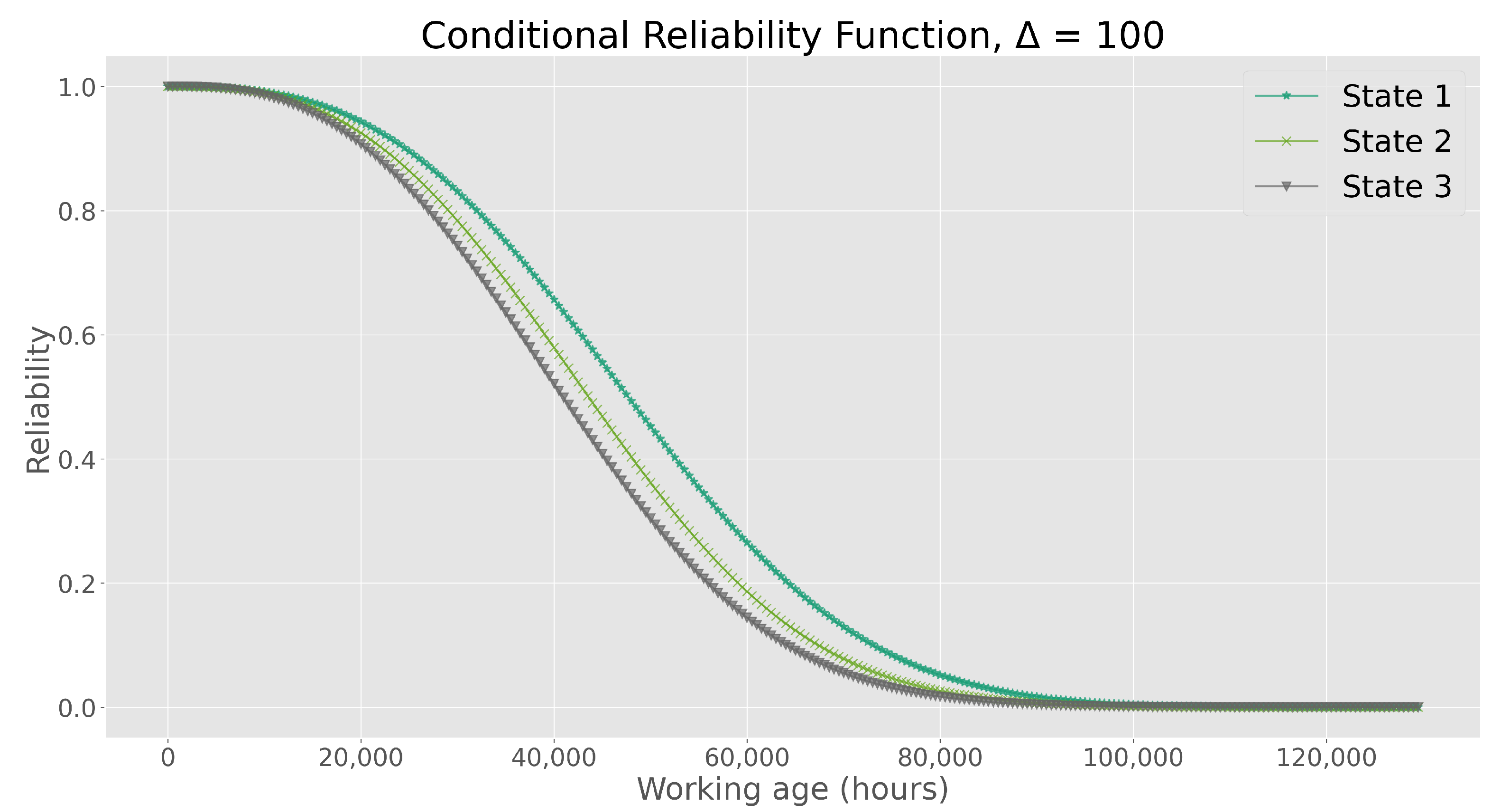
Therefore, three states are generated using the proposed method in [3], and the

Table 15. Transition Probability Matrix.

State	1	2	3
1	99.9917%	0.0050%	0.0033%
2	0.0049%	99.9828%	0.0123%
3	0.0024%	0.0048%	99.9929%

matrix is calculated. With this matrix, it is possible to obtain conditional reliability for each state (with $\mathrm{\Delta }=100$ and $t_{initial}=0$), as can be seen in Figure 2.

Then, Figure 2 shows the corresponding conditional reliability functions using the probability transition matrices as input to the aforementioned product property method. The reliability behavior for each state is similar. Consequently, State 1 corresponds to the state where the asset exhibits the highest reliability, followed by State 2 and then State 3, which present the lowest reliability over time.

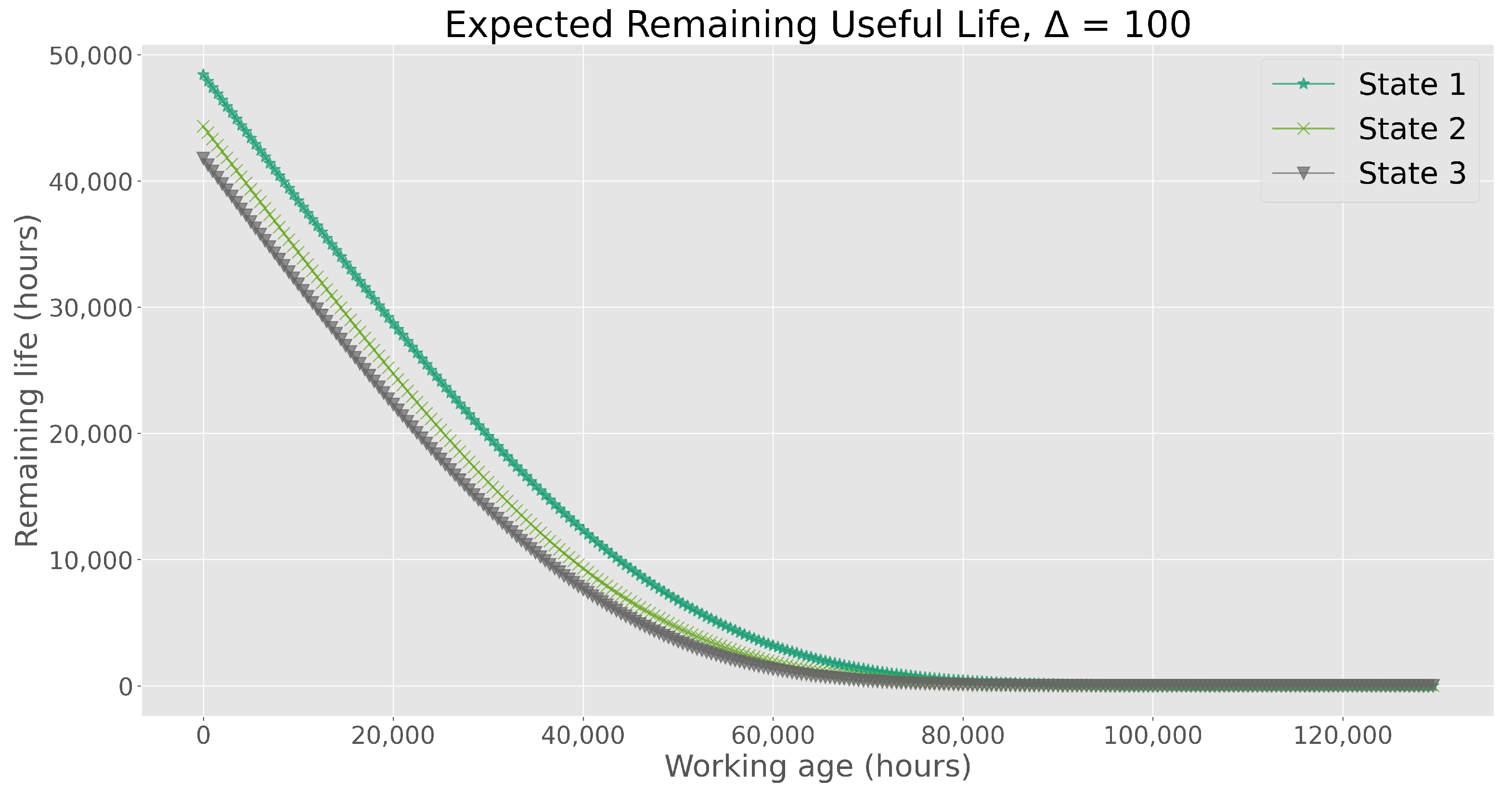
Figure 3 illustrates the remaining useful life (RUL) by incorporating the estimated conditional reliability functions as inputs for predictive analysis. This representation considers the progression of clustered covariate data across various states. Unsurprisingly, State 1 emerges as the optimal condition, characterized by a gradual decline in RUL from its peak, indicative of a smoother degradation process. Conversely, State 3 is identified as the least favorable clustered condition, exhibiting the most pronounced and aggressive deterioration throughout its operational lifespan.

With respect to the other component of the Predictive PHM Model (Equation (15)), i.e., the contribution of age to the risk rate, values of $\beta$ and $\eta$ align with their interpretation in conditional reliability and Remaining Useful Life (RUL), as evidenced in Figure 2 and Figure 3. In Table 8, it is observed that the value of $\beta$ is greater than one, indicating a stage of wear in the asset’s life cycle. This implies that the studied equipment is aging over the analyzed period. Characteristic life $\eta$ also aligns with the values of operating time. However, it is interesting to note that in the initial stages of the life cycle, the impact of the clustered condition is slightly more significant than the effect of age; that is, the difference in RUL between states is more noticeable.

In alignment with the PHM model, divergences in Remaining Useful Life (RUL) decrease during the later stages of the asset’s lifespan. This indicates that, over prolonged operational periods, the influence of time becomes more prominent as the overall condition of the asset undergoes significant degradation in advanced operating times.

In summary, the Genetic Algorithm (GA) exhibits greater robustness compared to IPOPT, even though GA falls short of achieving results as optimal as IPOPT concerning log-likelihood values (LL) and computational cost. It is important to notice that LL measures the goodness of fit of a statistical model, but p-values related to 95% confidence intervals for the estimated parameters are calculated as well. Introducing the Kaplan–Meier estimator as an upper bound yields superior results compared to scenarios without upper bounds, establishing it as a valuable technique for upper bound estimation. Additionally, Gradient Boosting with component-wise least squares (CWLS) as the base learner demonstrates robustness in providing reliable initial value estimates across all analyzed iterations. Hence, it is evident that addressing boundaries and employing a thoughtful initial value strategy is crucial for effectively solving this problem. Moreover, the estimation strategy introduced in this study enhances the robustness of Maximum Likelihood Estimation (MLE) optimization in the Weibull Proportional Hazard Model (PHM).

The data scaling methods improve performance of solver algorithms, reaching optimal solutions with less computational efforts. Additionally, the Gradient Boosting approach and the voting method of Random Forest (RF) are easily interpretable due to their intuitive operation. Furthermore, their calculation processes are straightforward to follow. However, the Component-Wise Least Squares (CWLS) method appears to outperform other methods for the considered optimization algorithms. Finally, as an illustrative example of attainable solutions, a transition matrix is calculated. Subsequently, the conditional reliability function and Remaining Useful Life (RUL) are estimated for each state, contributing to enhanced predictive analyses for Condition-Based Maintenance (CBM).

All the presented findings are derived from a real-world dataset within the electric industry, encountering typical data handling challenges such as missing values and non-ideal behaviors of the underlying data distributions—a common occurrence across various fields. To address these challenges, mixed semi/non-parametric algorithms are employed, capable of handling multiple variables with diverse behaviors and units. However, the multi-objective problem-solving approach proposed in this study may need further validation with additional covariates when diverse datasets from other capital-intensive scenarios are presented. Additionally, a dedicated study focusing on challenges related to parameter estimation and the integration of covariate bands calculation is essential to develop a robust and integrated Data-Driven multi-covariate Weibull Proportional Hazard Model (PHM).

5. Conclusions

This paper adopted new data-driven approaches for parameter estimation in the Weibull PHM context. Several Machine Learning methods were proven to estimate boundaries and starting/initial values for a non-convex problem, i.e., Cox’s partial likelihood with multiple covariates and Weibull distribution. Two optimization algorithms, a genetic algorithm (non-parametric) and an interior point optimizer (semi-parametric), were used to solve this non-convex problem, reaching feasible results in both cases. In addition, data scaling was analyzed, and the inclusion of Min–Max methods showed consistent MLE results when the max value was 1 and was better than the expert knowledge method (NS). So, regarding computational cost, data scaling simplifies the work for the optimization methods and helps to reach an outperformed MLE.

In conclusion, the proposed methodology establishes a novel framework for evaluating covariate weights and Weibull parameters by applying data-driven methodologies and advanced algorithms in scenarios when the boundaries assessment and seed values strategy are critical. This approach contributes to heightened robustness in non-convex log-likelihood optimization. Furthermore, data scaling helps the covariate data handling when different orders of magnitude and units are involved. Finally, it enhances the Proportional Hazards Model (PHM) by assessing multiple covariates under a Machine Learning approach, thereby offering a more interpretable model for the decision-making process in predictive maintenance.

In future work, one possible area of focus could be the validation and testing of the proposed methodology in a wider range of industrial applications. While the real-world case study in the electric power industry provides promising results, testing the methodology in other industries, such as transportation, energy, or mining, to evaluate its effectiveness and generalizability. Additionally, further research could explore integrating other advanced data-driven techniques to enhance the accuracy and reliability of RUL prediction in PHM models with multiple covariates. Finally, future work could also investigate using other probability distributions, such as log-normal or Gamma distributions, to model the failure data and compare their performance with the Weibull distribution.

References

1. Safaei, N.; Jardine, A.K. Aircraft routing with generalized maintenance constraints. Omega 2018, 80, 111–122. [Google Scholar] [CrossRef]
2. Maletič, D.; Maletič, M.; Al-Najjar, B.; Gomišček, B. An analysis of physical asset management core practices and their influence on operational performance. Sustainability 2020, 12, 9097. [Google Scholar] [CrossRef]
3. Godoy, D.R.; Álvarez, V.; López-Campos, M. Optimizing Predictive Maintenance Decisions: Use of Non-Arbitrary Multi-Covariate Bands in a Novel Condition Assessment under a Machine Learning Approach. Machines 2023, 11, 418. [Google Scholar] [CrossRef]
4. Nehring, M.; Knights, P.; Kizil, M.; Hay, E. A comparison of strategic mine planning approaches for in-pit crushing and conveying, and truck/shovel systems. Int. J. Min. Sci. Technol. 2018, 28, 205–214. [Google Scholar] [CrossRef]
5. Galar, D.; Kans, M. The impact of maintenance 4.0 and big data analytics within strategic asset management. In Proceedings of the Maintenance Performance and Measurement and Management 2016 (MPMM 2016), Luleå Tekniska Universitet, Luleå, Sweden, 28 November 2017; pp. 96–104. [Google Scholar]
6. Crespo, A.; Gómez, J.F.; Martínez-Galán, P.; Guillén, A. Maintenance management through intelligent asset management platforms (IAMP). Emerging factors, key impact areas and data models. Energies 2020, 13, 3762. [Google Scholar] [CrossRef]
7. Jardine, A.K.; Lin, D.; Banjevic, D. A review on machinery diagnostics and prognostics implementing condition-based maintenance. Mech. Syst. Signal Process. 2006, 20, 1483–1510. [Google Scholar] [CrossRef]
8. Cox, D.R. Regression models and life-tables. J. R. Stat. Soc. Ser. B (Methodol.) 1972, 34, 187–202. [Google Scholar] [CrossRef]
9. Jardine, A.K.; Tsang, A.H. Maintenance, Replacement, and Reliability: Theory and Applications; CRC Press: Boca Ratón, FL, USA, 2005. [Google Scholar]
10. Zheng, R.; Najafi, S.; Zhang, Y. A recursive method for the health assessment of systems using the proportional hazards model. Reliab. Eng. Syst. Saf. 2022, 221, 108379. [Google Scholar] [CrossRef]
11. Zheng, R.; Wang, J.; Zhang, Y. A hybrid repair-replacement policy in the proportional hazards model. Eur. J. Oper. Res. 2023, 304, 1011–1021. [Google Scholar] [CrossRef]
12. Zheng, R.; Makis, V. Optimal condition-based maintenance with general repair and two dependent failure modes. Comput. Ind. Eng. 2020, 141, 106322. [Google Scholar] [CrossRef]
13. Banjevic, D.; Jardine, A. Calculation of reliability function and remaining useful life for a Markov failure time process. IMA J. Manag. Math. 2006, 17, 115–130. [Google Scholar] [CrossRef]
14. Newby, M. Accelerated failure time models for reliability data analysis. Reliab. Eng. Syst. Saf. 1988, 20, 187–197. [Google Scholar] [CrossRef]
15. Wilson, C.M.; Li, K.; Sun, Q.; Kuan, P.F.; Wang, X. Fenchel duality of Cox partial likelihood with an application in survival kernel learning. Artif. Intell. Med. 2021, 116, 102077. [Google Scholar] [CrossRef] [PubMed]
16. Liu, H.; Makis, V. Cutting-tool reliability assessment in variable machining conditions. IEEE Trans. Reliab. 1996, 45, 573–581. [Google Scholar]
17. Xu, M.; Droguett, E.L.; Lins, I.D.; das Chagas Moura, M. On the q-Weibull distribution for reliability applications: An adaptive hybrid artificial bee colony algorithm for parameter estimation. Reliab. Eng. Syst. Saf. 2017, 158, 93–105. [Google Scholar] [CrossRef]
18. Vlok, P.; Coetzee, J.; Banjevic, D.; Jardine, A.K.; Makis, V. Optimal component replacement decisions using vibration monitoring and the proportional-hazards model. J. Oper. Res. Soc. 2002, 53, 193–202. [Google Scholar] [CrossRef]
19. Press, W.; Teukolsky, S.; Vetterling, W.; Flannery, B. Rational Function Interpolation and Extrapolation. In Numerical Recipes in C: The Art of Scientific Computing; Cambridge University Press: Cambridge, UK, 1994. [Google Scholar]
20. Mascarenhas, W.F. The BFGS method with exact line searches fails for non-convex objective functions. Math. Program. 2004, 99, 49. [Google Scholar] [CrossRef]
21. Lawless, J.F. Statistical Models and Methods for Lifetime Data; John Wiley & Sons: Hoboken, NJ, USA, 2011. [Google Scholar]
22. Smith, R.L. Weibull regression models for reliability data. Reliab. Eng. Syst. Saf. 1991, 34, 55–76. [Google Scholar] [CrossRef]
23. Zheng, R.; Zhou, Y. A dynamic inspection and replacement policy for a two-unit production system subject to interdependence. Appl. Math. Model. 2022, 103, 221–237. [Google Scholar] [CrossRef]
24. Liu, W.; Li, A.; Fang, W.; Love, P.E.; Hartmann, T.; Luo, H. A hybrid data-driven model for geotechnical reliability analysis. Reliab. Eng. Syst. Saf. 2023, 231, 108985. [Google Scholar] [CrossRef]
25. Hesabi, H.; Nourelfath, M.; Hajji, A. A deep learning predictive model for selective maintenance optimization. Reliab. Eng. Syst. Saf. 2022, 219, 108191. [Google Scholar] [CrossRef]
26. Mikhail, M.; Ouali, M.S.; Yacout, S. A data-driven methodology with a nonparametric reliability method for optimal condition-based maintenance strategies. Reliab. Eng. Syst. Saf. 2024, 241, 109668. [Google Scholar] [CrossRef]
27. Mofolasayo, A.; Young, S.; Martínez, P.; Ahmad, R. How to adapt lean practices in SMEs to support Industry 4.0 in manufacturing. Procedia Comput. Sci. 2022, 200, 934–943. [Google Scholar] [CrossRef]
28. Shinde, P.P.; Shah, S. A review of machine learning and deep learning applications. In Proceedings of the 2018 Fourth International Conference on Computing Communication Control and Automation (ICCUBEA), Pune, India, 16–18 August 2018; pp. 1–6. [Google Scholar]
29. Rajendra, P.; Girisha, A.; Gunavardhana Naidu, T. Advancement of machine learning in materials science. Mater. Today Proc. 2022, 62, 5503–5507. [Google Scholar] [CrossRef]
30. Rao, H.; Shi, X.; Rodrigue, A.K.; Feng, J.; Xia, Y.; Elhoseny, M.; Yuan, X.; Gu, L. Feature selection based on artificial bee colony and gradient boosting decision tree. Appl. Soft Comput. 2019, 74, 634–642. [Google Scholar] [CrossRef]
31. Wang, J.; Zhao, Z.; Liu, G.; Xu, H. A robust optimization approach of well placement for doublet in heterogeneous geothermal reservoirs using random forest technique and genetic algorithm. Energy 2022, 254, 124427. [Google Scholar] [CrossRef]
32. Paul, D.; Su, R.; Romain, M.; Sébastien, V.; Pierre, V.; Isabelle, G. Feature selection for outcome prediction in oesophageal cancer using genetic algorithm and random forest classifier. Comput. Med Imaging Graph. 2017, 60, 42–49. [Google Scholar] [CrossRef]
33. He, Y.; Wang, J.; Liu, X.; Wang, X.; Ouyang, H. Modelling and solving of knapsack problem with setup based on evolutionary algorithm. Math. Comput. Simul. 2023, 219, 378–403. [Google Scholar] [CrossRef]
34. Katoch, S.; Chauhan, S.S.; Kumar, V. A review on genetic algorithm: Past, present, and future. Multimed. Tools Appl. 2021, 80, 8091–8126. [Google Scholar] [CrossRef]
35. Cavallaro, C.; Cutello, V.; Pavone, M.; Zito, F. Machine Learning and Genetic Algorithms: A case study on image reconstruction. Knowl.-Based Syst. 2024, 284, 111194. [Google Scholar] [CrossRef]
36. Chen, C.; Liu, Y.; Wang, S.; Sun, X.; Di Cairano-Gilfedder, C.; Titmus, S.; Syntetos, A.A. Predictive maintenance using cox proportional hazard deep learning. Adv. Eng. Inform. 2020, 44, 101054. [Google Scholar] [CrossRef]
37. Klein, J.P.; Moeschberger, M.L.; Klein, J.P.; Moeschberger, M.L. Nonparametric estimation of basic quantities for right-censored and left-truncated data. In Survival Analysis: Techniques for Censored and Truncated Data; Springer: New York, NY, USA, 2003; pp. 91–138. [Google Scholar]
38. Satten, G.A.; Datta, S. The Kaplan–Meier estimator as an inverse-probability-of-censoring weighted average. Am. Stat. 2001, 55, 207–210. [Google Scholar] [CrossRef]
39. Ridgeway, G. The state of boosting. Comput. Sci. Stat. 1999, 31, 172–181. [Google Scholar]
40. Friedman, J.H. Greedy function approximation: A gradient boosting machine. Ann. Stat. 2001, 29, 1189–1232. [Google Scholar] [CrossRef]
41. Friedman, J.H. Stochastic gradient boosting. Comput. Stat. Data Anal. 2002, 38, 367–378. [Google Scholar] [CrossRef]
42. Hothorn, T.; Bühlmann, P.; Dudoit, S.; Molinaro, A.; Van Der Laan, M.J. Survival ensembles. Biostatistics 2006, 7, 355–373. [Google Scholar] [CrossRef]
43. Breiman, L. Bagging predictors. Mach. Learn. 1996, 24, 123–140. [Google Scholar] [CrossRef]
44. Biró, T.S.; Néda, Z. Gintropy: Gini index based generalization of entropy. Entropy 2020, 22, 879. [Google Scholar] [CrossRef]
45. Stute, W. Consistent estimation under random censorship when covariables are present. J. Multivar. Anal. 1993, 45, 89–103. [Google Scholar] [CrossRef]
46. Jardine, A.; Anderson, P.; Mann, D. Application of the Weibull proportional hazards model to aircraft and marine engine failure data. Qual. Reliab. Eng. Int. 1987, 3, 77–82. [Google Scholar] [CrossRef]
47. Holland, J.H. Adaptation in Natural and Artificial Systems: An Introductory Analysis with Applications to Biology, Control, and Artificial Intelligence; MIT Press: Cambridge, MA, USA, 1992. [Google Scholar]
48. Peiravi, A.; Ardakan, M.A.; Zio, E. A new Markov-based model for reliability optimization problems with mixed redundancy strategy. Reliab. Eng. Syst. Saf. 2020, 201, 106987. [Google Scholar] [CrossRef]
49. Wächter, A.; Biegler, L.T. On the implementation of an interior-point filter line-search algorithm for large-scale nonlinear programming. Math. Program. 2006, 106, 25–57. [Google Scholar] [CrossRef]
Figure 1. Flow chart of the proposed model.
Machines 12 00060 g001
Figure 2. Conditional reliability function for the case study.
Machines 12 00060 g002
Figure 3. Remaining useful life for the case study.
Machines 12 00060 g003