Abstract
Flexible shrouded blades are commonly adopted in the last stages of steam turbines where complicated dynamical behavior can be induced by dry friction force generated on contacting interfaces between adjacent shrouds and the geometric nonlinearity due to the structural flexibility of the blades. In this paper, combination resonance caused by contact and friction forces generated on shroud interfaces is investigated, which is a concurrence of 1:3 internal resonance involving the first and second modes in the flapwise direction and the primary resonance of the first flapwise mode. The stiffness and damping at the contact interface are obtained by linearizing the contact and friction forces between shrouds through the harmonic balance method. The vibrating blade is modeled as a beam with a concentrated mass of which the responses under the combination resonance are solved through the multiple-scale method. Sensitivities of response with respect to the angle of shrouds, contact stiffness and rotation speed are illustrated, and the influences of these parameters on the periodicity and amplitudes of steady responses are demonstrated. The parametric regions where the combination resonance occurs are pointed out. Finally, parametric analyses are presented to show how the amplitude–frequency relation of the multiple-scale solutions under the combination resonance vary with detuning and design parameters. The present research provides a designing basis for improving the dynamic performance of flexible shrouded blades and suppressing vibrations of blades by adjusting structural parameters in practical engineering.
1. Introduction
Shrouds have been widely used by developers of multi-stage steam turbines to dissipate vibratory energy and reduce the stress of rotating bladed blisks for the purpose of improving their structural reliability [1]. To ensure the constant flow rate of the steam, the blades mounted on the last-stage blisk are generally designed to be the longest with considerable structural flexibility, which causes an effect of geometric nonlinearity that cannot be ignored. On the other hand, there exists contact and dry friction on the contacting interfaces between adjacent shrouds, which intensifies the nonlinear characteristics as far as the dynamic of the shrouded blades is concerned.
Various studies were published previously devoted to modeling the shrouded blade of turbines, covering the topics of modeling of blades as well as the contact force between adjacent shrouds. Single-blade modeling was adopted to understand the dynamical properties of flexible turbine blades [2,3]. In some publications, the interaction between the reference blade and the adjacent blades [4,5,6] was considered, while a few studies were aimed at the vibration of the whole blade disk [7]. Zhou et al. [8] investigated the transverse vibration of composite blades of a wind turbine using a generalized Timoshenko beam. Slender blades that resembled the beam model and a rigid disk were integrated into a continuous model by Shadmani [9] in modal analysis of a turbine blisk. As for the contacts between adjacent shrouds, various models were published for evaluating the inter-shroud action of friction and contact. The effects of macro- and micro-slip between the neighboring blades were established by Griffin [10] and later publications such as [11,12]. Later, Yang and Menq established a special model to predict the resonance of structural response possessing a three-dimensional frictional constraint [13]. Nan et al. [14] translated the contact and friction that acted on the shroud interfaces into an equivalent stiffness as well as damping by means of the harmonic balance method.
In essence, the contact between the shrouds is physically nonlinear and has been regularly simplified as a piecewise linear function of the blade motion. In the view of dynamics, such contact force is attributable to complicated behaviors, e.g., self-excited vibrations, bifurcation of motion, chaos and switch of stability [15]. He et al. [16] proposed a full set of blades subjected to friction and impact forces due to shroud contacting and demonstrated various types of periodic, quasi-periodic and even chaotic motions of the blades. He et al. [17] studied the interaction of bending and torsional vibration of blades, considering the rub and impact between shrouds. As for the nonlinear dynamics of full blisks, achievements were made in mistuned disks, nonlinear resonance frequencies and localization phenomena [18,19,20,21,22,23].
For the combination resonance of the turbine blade, most of the existing research attended to the internal resonance [24,25,26], primary resonance [27,28] or combination resonance with both internal and sub- or super-harmonic responses [29,30,31]. A few publications were dedicated to the combination resonance consisting of the internal and primary resonances of the flexible turbine blade. Li et al. [32] investigated the nonlinear vibration of a blade simultaneously undergoing two resonances (i.e., internal as well as primary), considering aerodynamic force, damping and structural nonlinearity. Yuan and Wang studied internal resonance, primary resonance and the combined multiple modal resonances of a blade [33], where they demonstrated the contribution of primary and internal resonances to the combination resonance in terms of frequencies and energy. It is worth pointing out that, despite the existent works on the nonlinear vibrations of bladed blisks, the combination resonance induced by contact and friction between neighboring blades has yet to be thoroughly understood. Such understanding will provide a better understanding of the dynamical behaviors of flexible shrouded blades and how shroud design influences the blade vibration under the situation of combination resonance.
In the present study, the dynamics of a flexible blade mounted with a shroud are investigated, focusing particularly on the combination resonance of blade vibration that is induced by the contact as well as friction forces applied on the shroud. Firstly, the equivalent stiffness and damping of the shroud due to the normal contact as well as the friction are obtained through the method of harmonic balance, and the blade is simplified as one single continuous beam attached by a concentrated mass. A steady response under the combination resonance is presented through the multiple-scale method. Afterward, influences of design parameters on periodicities and amplitudes are demonstrated for the steady responses. Jumping of amplitude due to the primary resonance and the transfer of vibration energy between resonance modes excited by the internal resonance are pointed out. Finally, amplitude–frequency curves of the multiple-scale solutions under the combination resonance are derived. Parametric analyses are presented to show the effect of detuning and key design parameters on the first and second flapwise modes.
2. Governing Equations of Flexible Shrouded Blade
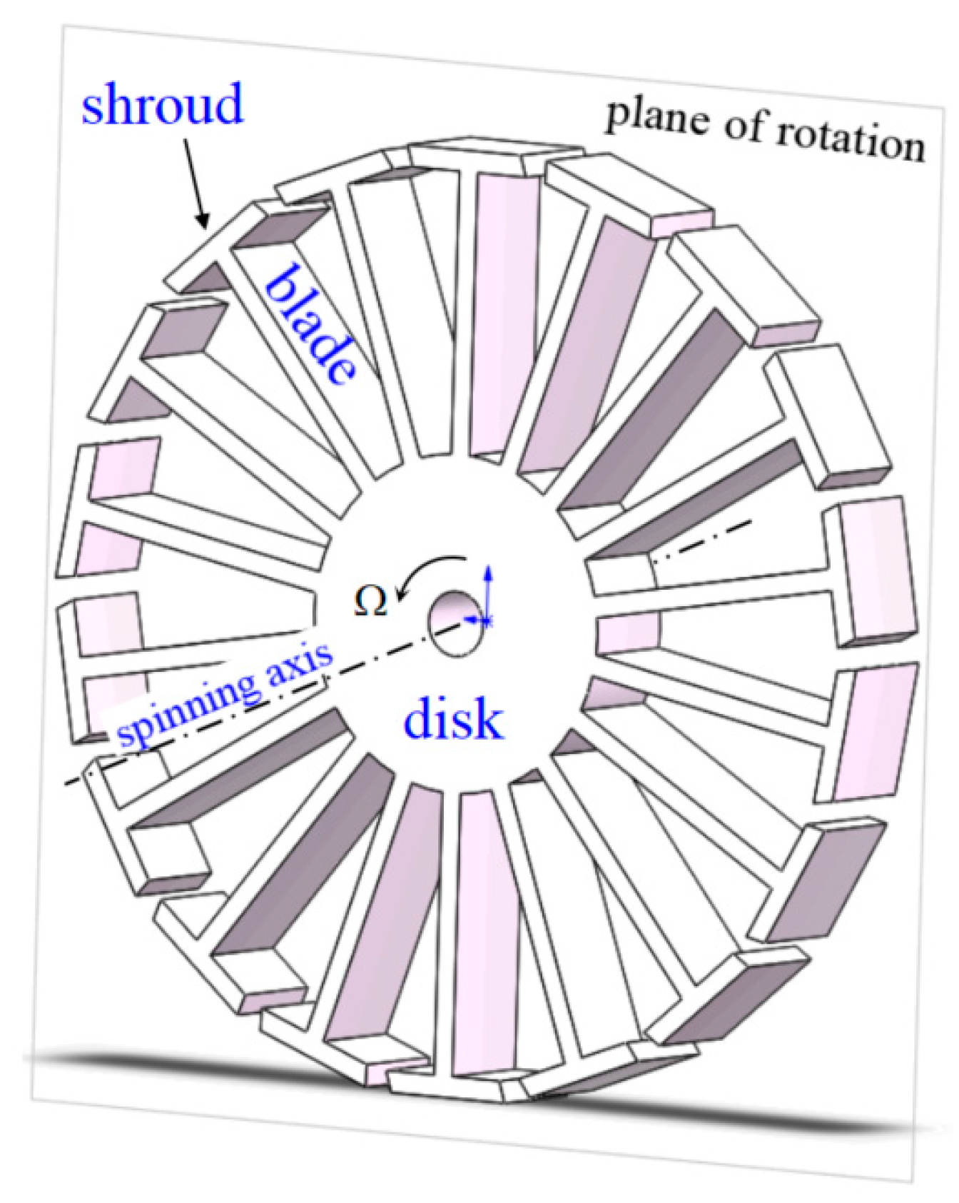
Figure 1 depicts the sketch of a perfectly tuned, rotating shrouded disk that is commonly used in steam turbines. For such a blisk, all of the shrouded blades are mounted circumferentially and separated in equal space [34]. Hence, the blisk can be considered to have a cyclic symmetry. In addition, the blades of the final stage of the turbine generally have a large span size to ensure the constant flow rate of the working medium, which will enhance the flexibility of the blade.
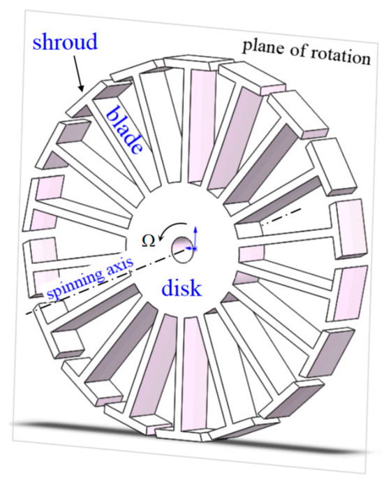
Figure 1.
Mechanical model of shrouded rotating disk.
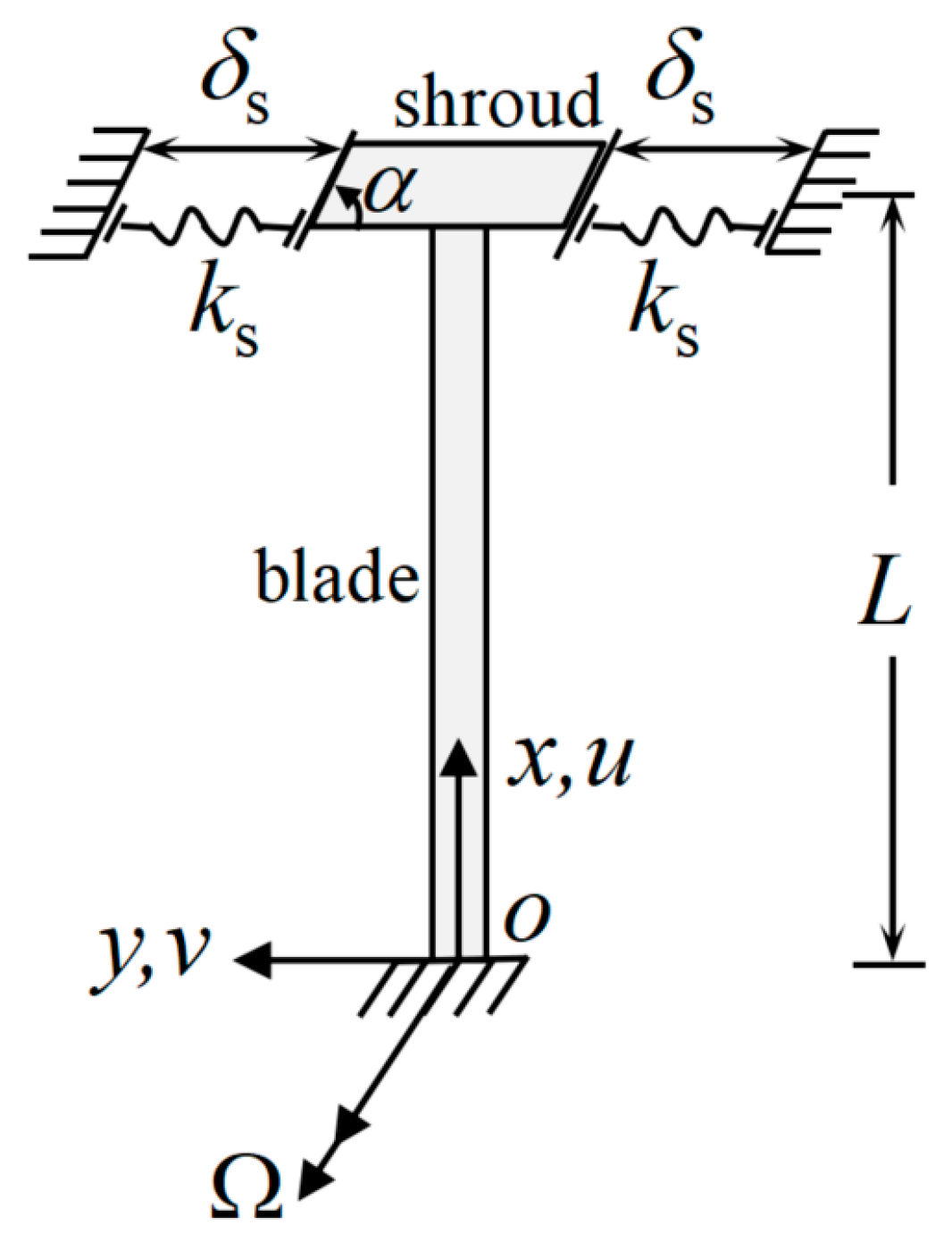
To focus on the overall dynamics of the blade, a macro-slip model is adopted in the present work. The dimension of the shroud mounted at the tip of the blade is small compared with the blade length and is generally rigid as opposed to the long and flexible blade, which can be further treated as a single mass point. The normal contact force between the adjacent shrouds is modeled by a linear spring [16]. Accordingly, the flexible shrouded blade is modeled as a beam with an attached mass that is placed at the tip of the blade, as shown in Figure 2. A Cartesian frame can be set up for the blade with the origin placed at the center of gravity of the root and three axes of x (axial direction), y (flapwise direction) and z (edgewise direction). α represents the tilting angle of the shroud, and Ω is the rotation speed. L is the length of the blade. and are contact (normal) stiffness and the circumferential gap between shrouds, respectively.
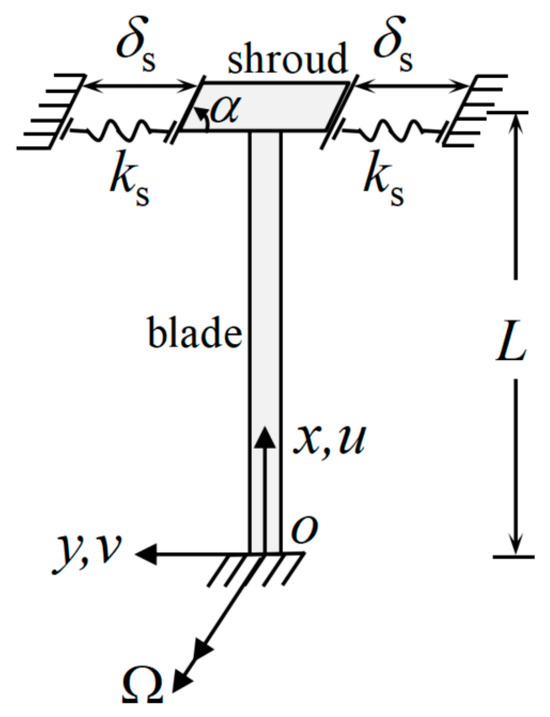
Figure 2.
Sketch of a flexible shrouded blade.
2.1. Dynamic Model of Contact between Adjacent Shrouds
Prior to deriving the governing equation of the blade motion, it is necessary to describe the contact action between adjacent shrouds, which is a contribution to the nonlinear dynamics and combination resonance. Hereafter, the equivalent stiffness and damping of the normal and friction between adjacent shrouds are established through the method of harmonic balance.
In this research, the contact force is presumed to change as a piecewise linear function of the relative displacement of two adjacent shrouds, whereas friction carries typical nonlinear characteristics. The states of contact (e.g., separation, stick or slip) depend upon relative displacements in both normal and tangential directions.
In Figure 3, the non-conservative forces on the shroud are aerodynamic force (Q), normal contact force () and friction (), where
with being the amplitude and l the number of guided vanes of the upstream inlet [27].
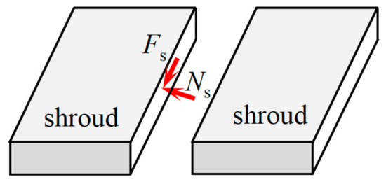
Figure 3.
The sketch of aerodynamic, normal and friction forces of the shroud.
The flapwise displacement of the blade, v, can be assumed as [14]
where B and ϕ stand for the amplitude and phase angle of displacement v, respectively. Then, the contact force between two adjacent shrouds is modeled as
As for the friction force between two neighboring shrouds, there are two possible situations during one cycle of the vibration based on the change in the normal force when the macro-slip model is adopted: (1) is not zero and time varies during shroud contacting, and (2) is zero when two shrouds separate. The hysteretic loop of the friction force changes along with the tangential relative displacement are depicted in Figure 4. Different from the hysteretic loop of the friction in [14], the influence of the normal force on sliding friction is considered in this paper.

Figure 4.
Hysteretic loop of friction versus tangential relative displacement.
As depicted in Figure 4, the friction force between shrouds starts from point A () and changes clockwisely according to the hysteresis loop. Section AB corresponds to the phase of static friction. Then, from point B () to point C (), the blade begins to slide towards the opposite direction. The segment of BC corresponds to the phase of sliding friction. The separation of adjacent shrouds takes place at point C, and the friction declines to zero at D (). Subsequently, continues to decrease, and the state of friction moves from D to D′ () where the blade starts to contact the blade from the other side. Section D′E′ also corresponds to the phase of static friction, where the blade begins to slide at point E′ (). After that, the negative reaches the maximum at A′ (). Notably, the section A′A in the loop is symmetric with section AA′.
Based on the aforementioned hysteretic behavior, the friction force can be modeled in terms of the state of contact between adjacent blades:
where and μ are shear stiffness and the friction coefficient of the contact surface of the shroud. , and are the phase angles of the friction force, defined as
To facilitate the dynamical analysis in the present study, the method of harmonic balance (HBM) [35] is used to simplify contact (normal) and friction forces to obtain the stiffness and damping at the shroud surface. For this purpose, one linearizes as
where
Based on Equation (3), the contribution of the blade velocity to the contact force is negligible; hence, one assumes
The friction force between adjacent shrouds can be expressed as
where and represent the stiffness and damping of , respectively.
2.2. Governing Equations of Blade Vibration
The blade in the present study is modeled as a beam attached by a concentrated shroud mass at the tip of the blade. For blades carrying small installation angles, their torsional rigidities are sufficient; hence, the twisting movement of the rotating blade can be effectively neglected. Thus, the edgewise deformation of the blade caused by the torsion should be neglected. Additionally, the dynamic spanwise (axial) displacement can be described as minor as opposed to the pre-stretching caused by centrifugal load on the blade [32]. Therefore, the interaction between the flapwise and axial motions is fulfilled by means of the centrifugal stiffening upon lateral vibration frequencies. Based on Figure 2, the equation of the blade flapwise vibration is established, which reads
where v = v(x,t) is the dynamic displacement of the blade in the flapwise. u = u(x) is the spanwise (axial) displacement generated by centrifugal force of the blade. The EI and EA are bending and tensile stiffnesses of the blade, respectively. represents the linear mass density of the blade. is the mass of shroud. The term is the outcome of geometric nonlinearity due to the structural flexibility of the blade, and is the Dirac function of x. The overhead dot and prime represent the partial derivatives of a physical quantity with respect to time t and x, respectively, i.e.,
Subsequently, the flapwise displacement of the blade is decomposed in the modal space
where stands for the mode shape of order k of the beam under given boundary conditions in the flapwise direction, and are the generalized (modal) coordinates of . Thus, Equation (13) can be simplified using the Galerkin method considering the first- and second-order modal coordinates, as
where , , and are defined in Equations (A1)–(A8), Appendix A. Further, Equation (16) can be rewritten with the introductions of non-dimensional notations:
such that one has the compact governing equations
where , , and are defined in Equations (A9)–(A15), Appendix A.
3. Multiple-Scale Solutions under Combination Resonance
The multiple-scale method will be adopted in this section for solving Equation (18). To construct the analytical solution of the problem, a small, artificial bookkeeping parameter is introduced to order the quantities of dynamic displacements, damping and aerodynamic forces before they are inserted into Equation (18). Thus, one has
Herein, the regular scale of time is replaced with three temporal scales, i.e.,
Then, is expanded using the power series of and the new scales
Let and substitute Equations (19) and (21) back to Equation (18), then equate their same orders of . In doing so, one obtains
where .
For Equation (22), let us assume that
and then substitute these back to Equation (23) to obtain
which further leads to
The highest can be evaluated through the perpetual term of Equation (24).
A particular type of combination resonance is of present interest, i.e., when a particular internal resonance takes places with (“1:3”). To be specific, the frequencies of the first-order flap mode are triple the second-order flapwise frequency, and alongside, there is a primary resonance of the first flapwise mode (i.e., ). Under this situation, one can assume that . By introducing new phases , , one obtains the equations of motion for the amplitudes of
and also for the phases of the motion
The steady solutions for these responses are determined through vanishing the right sides of Equations (28)–(31), which correspond to the fixed-point states of amplitudes of the first and second flapwise modes as well as their phases. The stability of the steady motion can be evaluated in terms of the eigenvalues of the following Jacobian matrix of the fixed points
where the components of J are provided in Equations (A16)–(A19), Appendix A. The response is said to be asymptotically stable if all of the eigenvalues possess negative real parts.
Afterwards, the approximations of and can be obtained as
When the combination resonance happens, the steady responses are determined through conditions
Nonetheless, are constrained by the inequalities
in order to assure the absolutes of and in Equations (28)–(31) are not greater than 1.
In the solution procedure, a simulation is implemented using the Runge–Kutta method with variable step size to obtain numerical results of Equation (18) and the analytical results of the transient system (28)–(31), whereas the analytical steady Equations (35)–(36) are solved through Newton’s iteration method. Nevertheless, it is necessary to solve the amplitude of the steady response (i.e., B in Equation (2)) via iterations before the solution of the governing equations begins. Such an iterative process for B is described in Appendix B.
4. Nonlinear Dynamics and Combination Resonance of Shrouded Blade
A flexible shrouded blade is used for examples and discussions. The major parameters involving the blade design and operation are provided in Table 1. The natural frequencies are and for the first-order and second-order modes in the flapwise direction. However, these frequencies become and when one considers the action of contact and friction on the shroud. The condition for concurrence of an internal resonance of type 1:3 between the two flapwise modes and the primary resonance of the first flapwise mode is expected when considering the aforementioned contact and friction.

Table 1.
Major parameters of the blade.
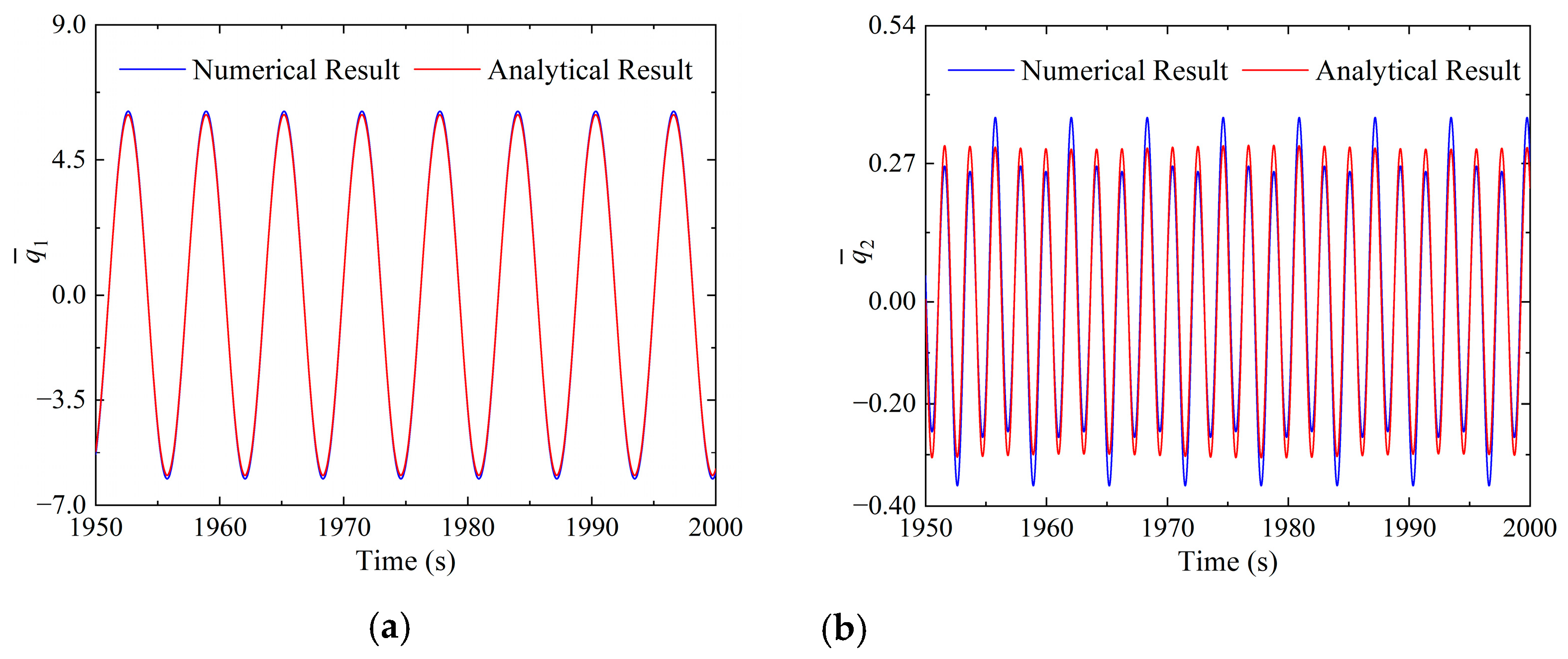
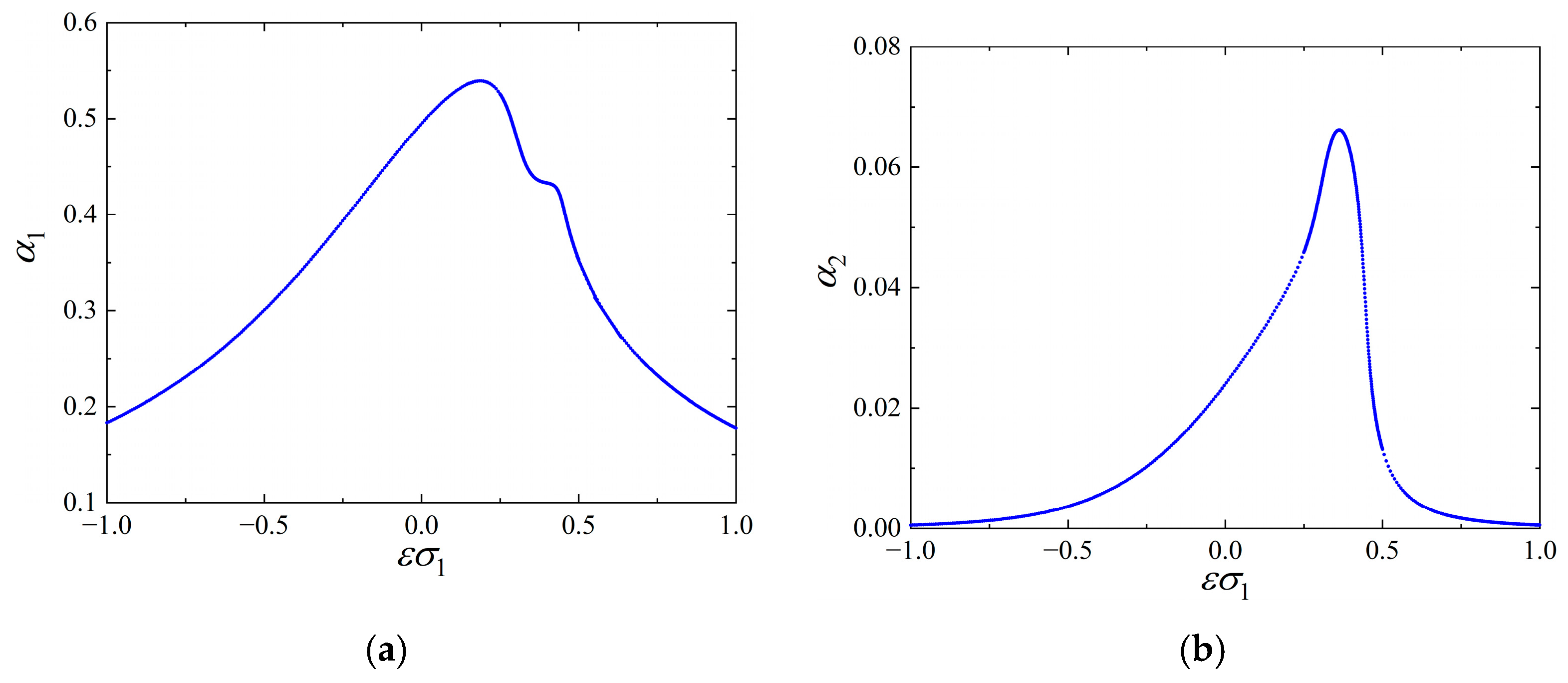
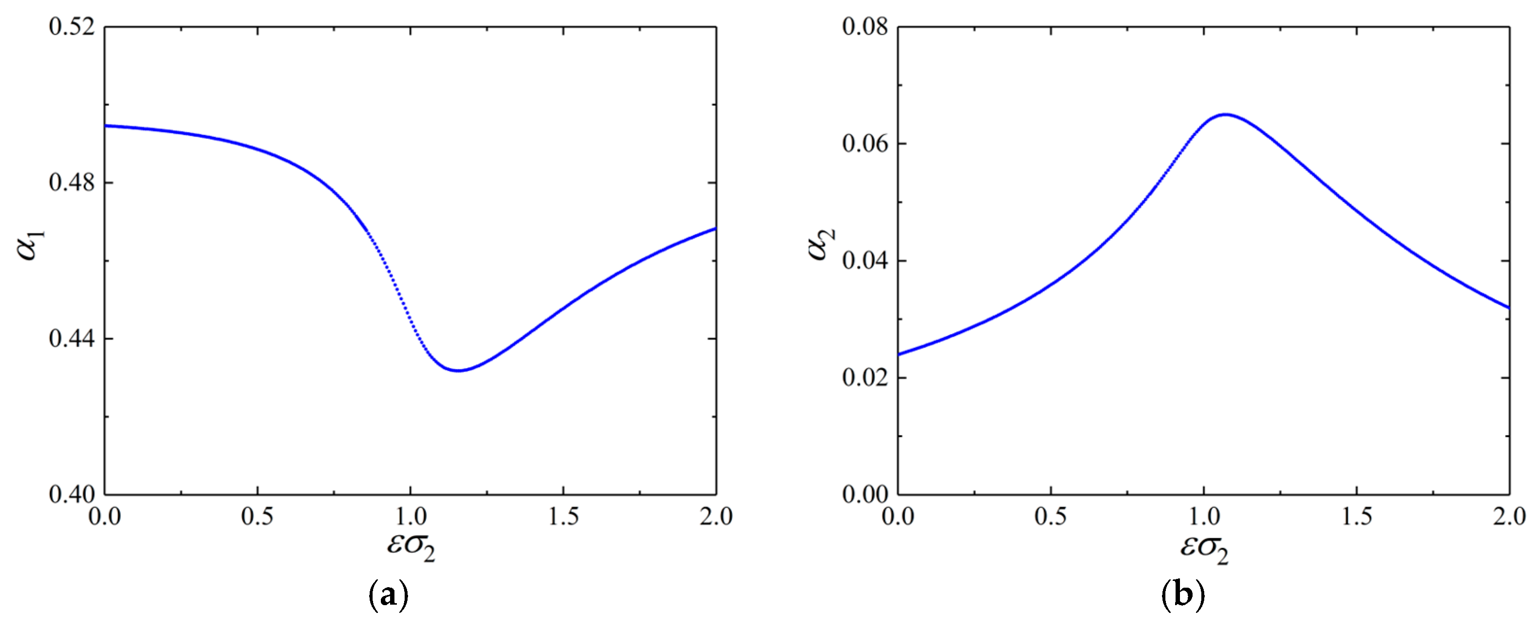
To validate the proposed method, the steady responses of the original Equation (18) are solved with the analytical, multiple-scale results through Equations (33)–(34), which are obtained by computing Equations (28)–(31). As shown in Figure 5, these analytical solutions are found in good agreement with their numerical counterparts. Their discrepancies are inevitable, since higher order terms have been excluded from multiple-scale-based expansions, and they appear more noticeable for the second flapwise mode than the first. In summary, the proposed modeling and approximate approach are applicable for steady-response solutions of the shrouded blade in the situation of combination resonance.
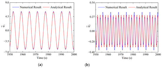
Figure 5.
Analytical and numerical steady responses. (a) First flapwise mode and (b) second flapwise mode.
4.1. Steady Responses of Flexible Shrouded Blade
For flexible blades, the tilting angle and contact stiffness of the shroud are key to the contact status of adjacent shrouds. Further, the blade rotating induces centrifugal load and the subsequent spinning softening that reduces the axial stiffness of the blade. In the following, the original governing Equation (18) is solved with various tilting angle, contact stiffness and rotation speed values to reflect their influence on the response.
4.1.1. Effect of Tilting Shroud
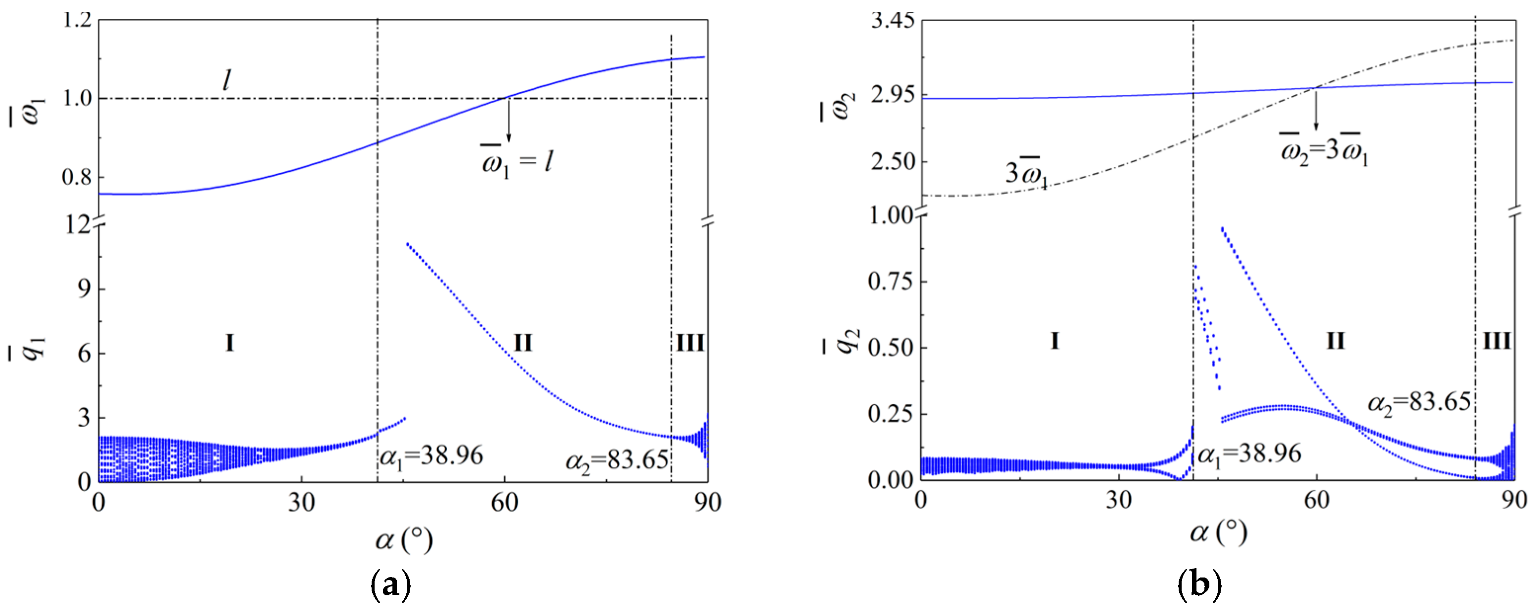
The bifurcation diagram of the blade vibration is demonstrated using the tilting angle of shroud varying between 0 and 90°, Figure 6. Based on the characteristic of the steady response of the first-order and second-order flapwise modes, the range of the tilting angle is divided into three stages, denoted by stage-I, -II and -III, respectively, with = 38.96° and = 83.65° being the dividing points that separate the stages.
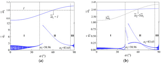
Figure 6.
Bifurcation of the blade under variable . (a) and (b) .
The steady responses of the first-order mode under variable are shown in Figure 6a. In stage-I, is quasi-periodic motion. Then, becomes periodic-1, and the resonance peak of the primary resonance, , can be observed in stage-II. In addition, the jumping of the amplitude and the phenomenon of so-called “hardening” can be seen for stage-II, owing to the geometric nonlinearity originating from Equation (13). Finally, for stage-III, is converted back to quasi-periodic motion. It is worthwhile to mention the curving of the resonance summit towards the side where the ratio between the frequency of external excitation and natural frequency, , goes up is defined as the hardening spring. In these cases, the jumping of the amplitude and the unstable motion appear in the steady response. However, the steady response is obtained through the Runge–Kutta method in Section 4.1, by which only the stable motion can be observed.
Corresponding to the first flapwise mode, the periodicity of is the same as that of in stage-I and -III, but represents 3-periodic motion in stage-II, Figure 6b. In addition, the jumping of amplitude and the hardening phenomenon caused by the primary resonance can also be observed in stage-II. This is because the primary and internal resonances concur as and , which leads to the desired combination resonance. Therefore, the primary resonance is also observed in due to the exchanges in energy between the first-order and second-order modes in the flapwise direction.
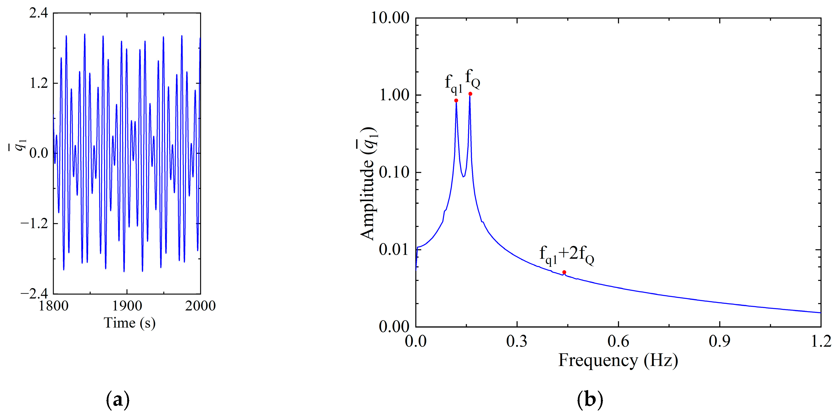
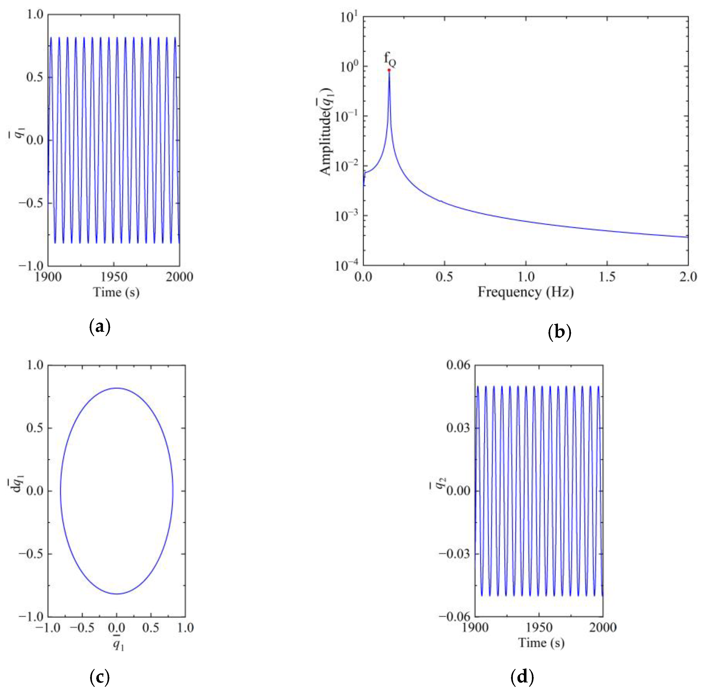
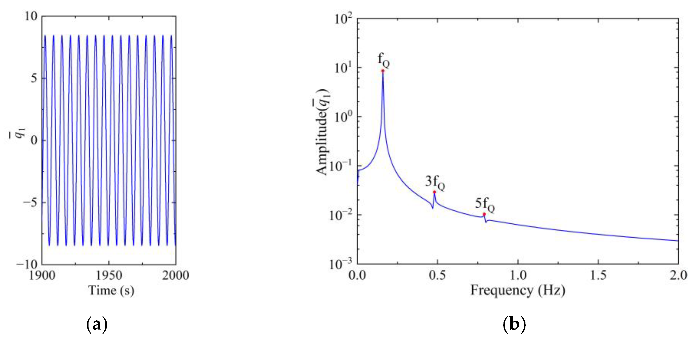
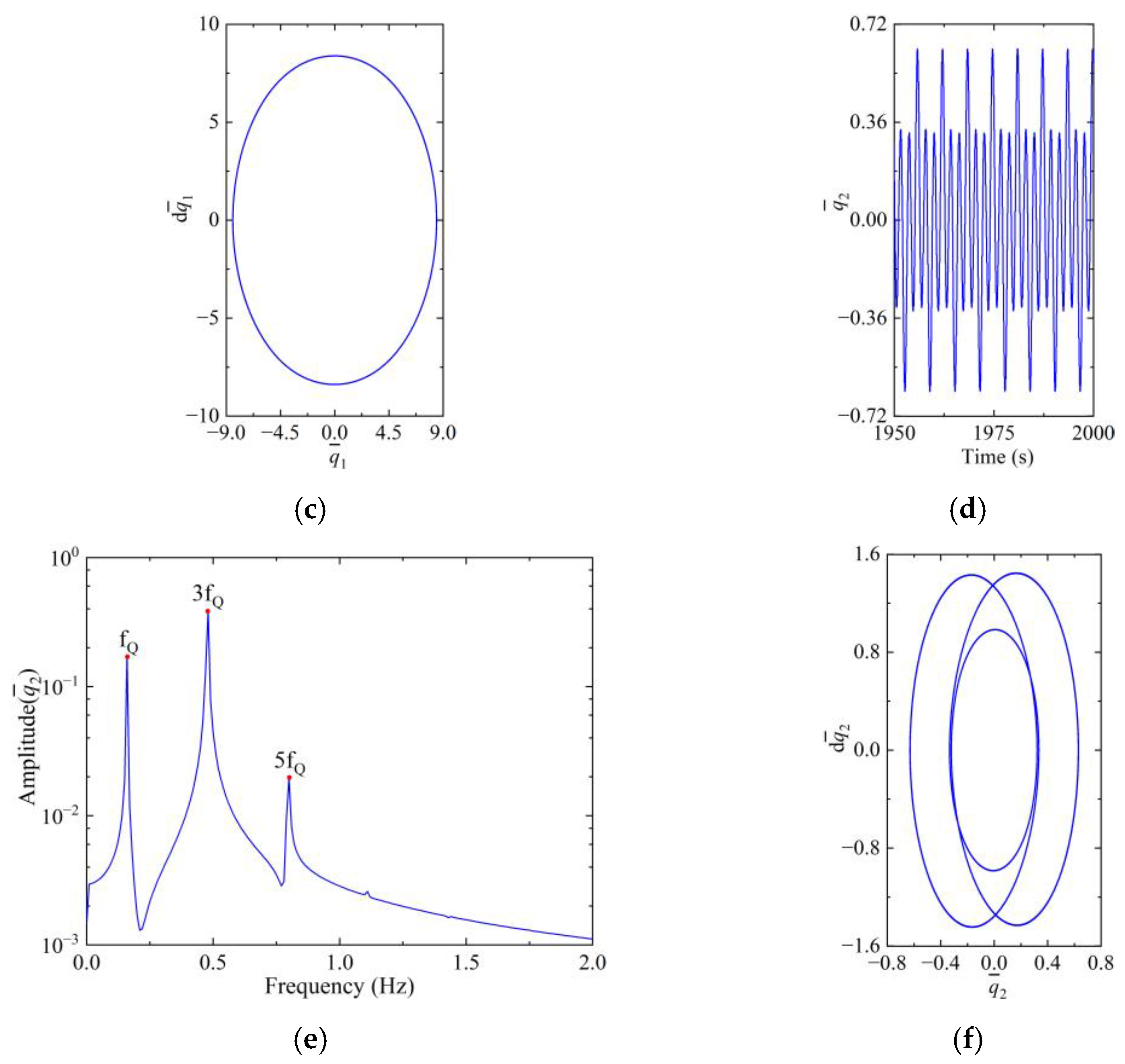
Further examinations are made focusing on the blade vibration carrying four different tilts angle of shrouds: 4.07° (in stage-I), 40.28°, 40.28° (in stage-II) and 85.48° (in stage-III), and the results are provided through Figure 7, Figure 8, Figure 9 and Figure 10. As found in Figure 7, both and are quasi-periodic motions with spectra containing the aerodynamic frequency , the first flapwise frequency and the combined frequencies of , and . Further, the amplitude of is synchronous and π is out-of-phase against the amplitude of . This implies that it is likely to have internal resonance when is small, since the curving of the resonance summit occurs as the blade appears hardened in this scenario. The energy carried by the first order flapwise mode is able to transmit to the second flapwise mode and vice versa.

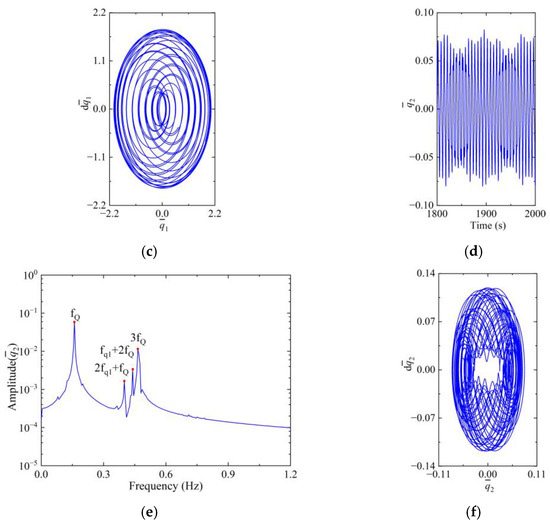
Figure 7.
Steady responses of the blade with α = 4.07°. (a) Time history, (b) frequency spectra and (c) phase diagram of ; (d) time history, (e) frequency spectra and (f) phase diagram of .


Figure 8.
Steady responses of the blade with α = 40.28°. (a) Time history, (b) frequency spectra and (c) phase diagram of ; (d) time history, (e) frequency spectra and (f) phase diagram of .

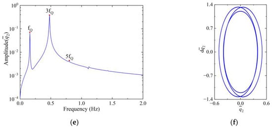
Figure 9.
Steady responses of the blade with α = 44.81°. (a) Time history, (b) frequency spectra and (c) phase diagram of ; (d) time history, (e) frequency spectra and (f) phase diagram of .
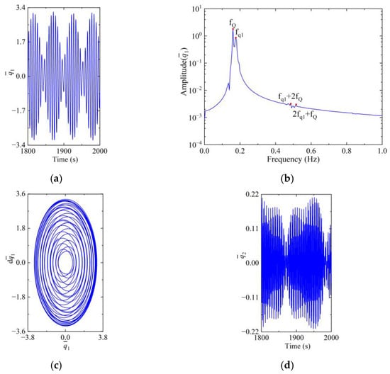
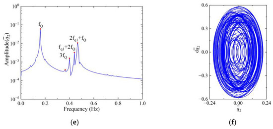
Figure 10.
Steady responses of the blade with 85.48°. (a) Time history, (b) frequency spectra and (c) phase diagram of ; (d) time history, (e) frequency spectra and (f) phase diagram of .
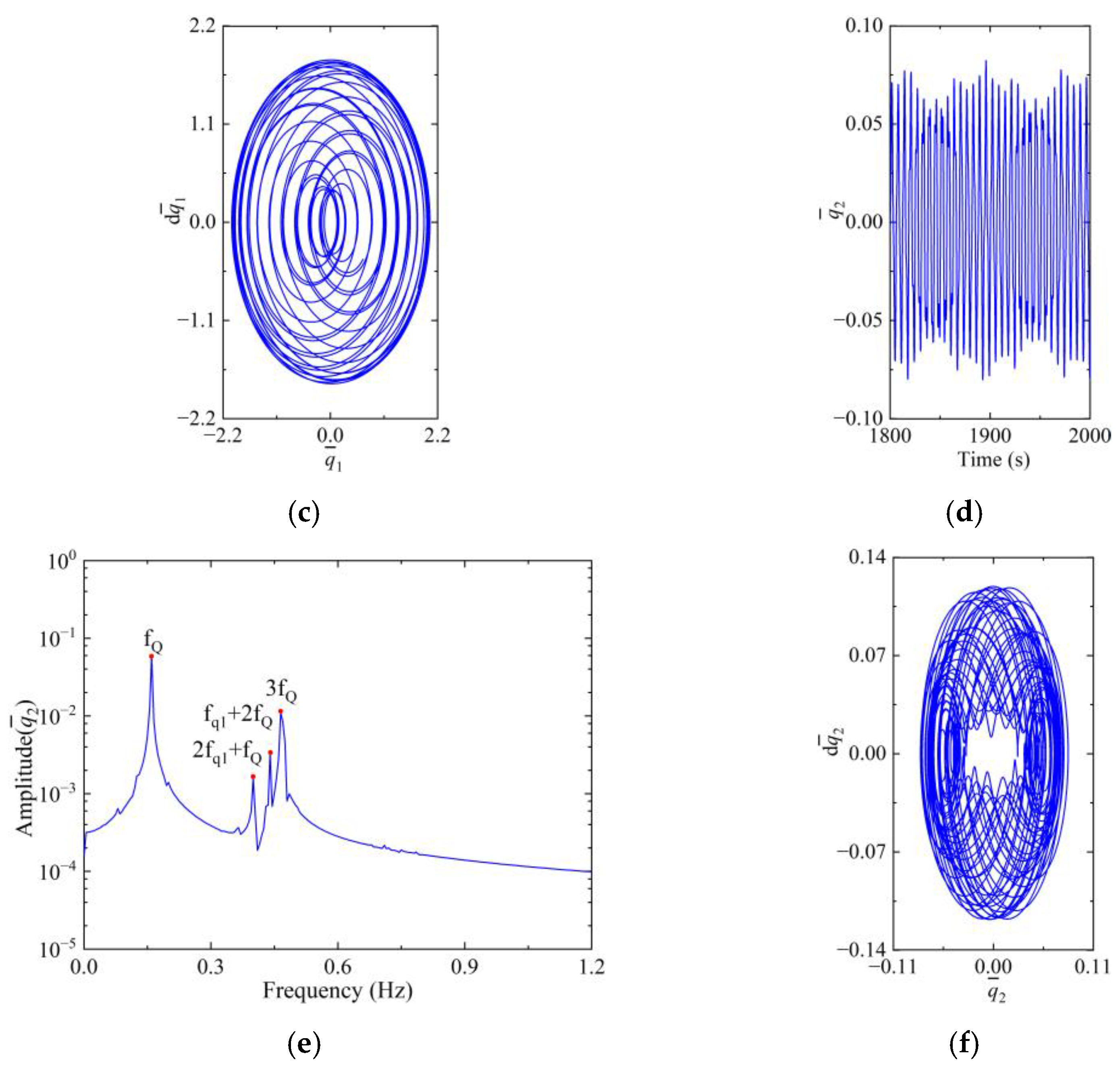
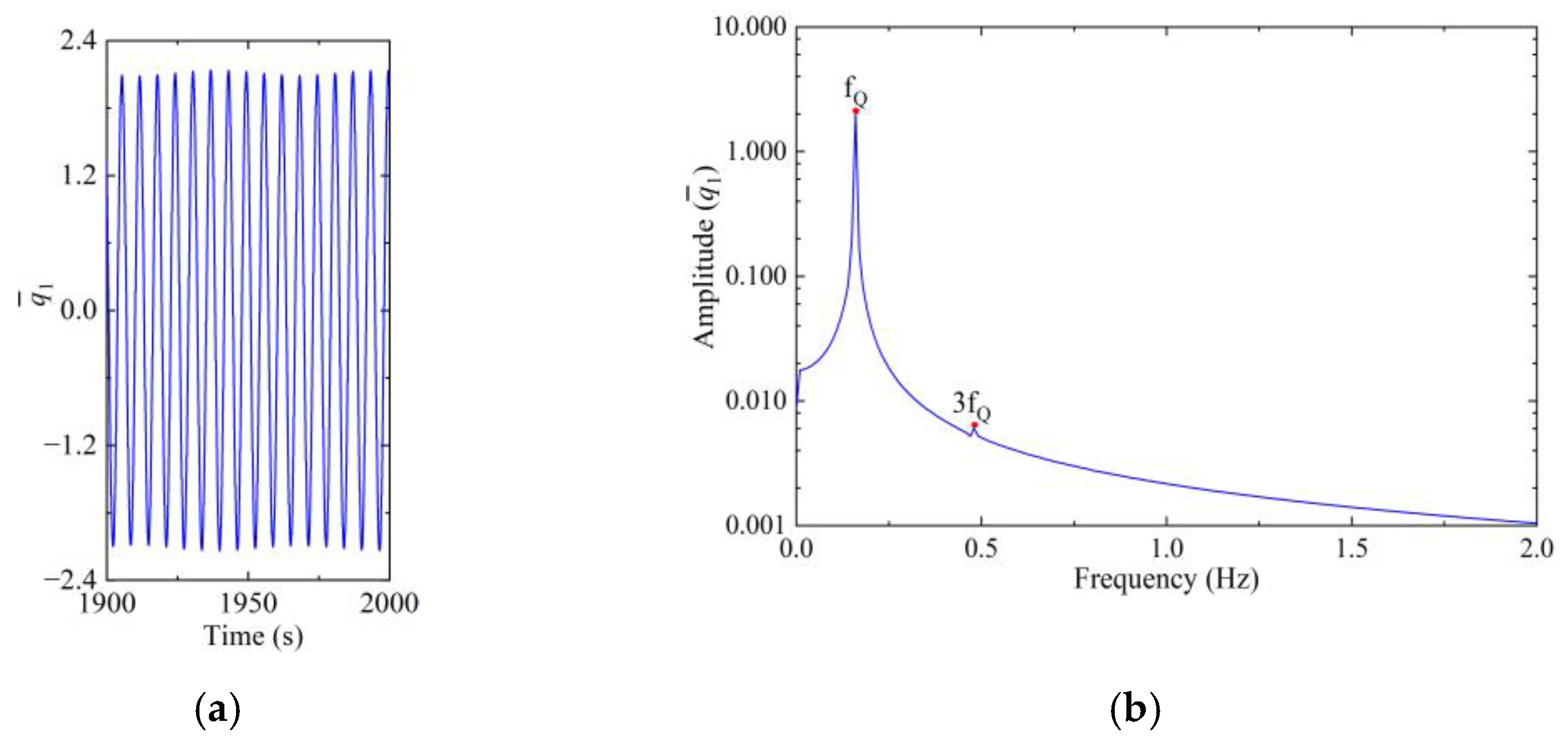
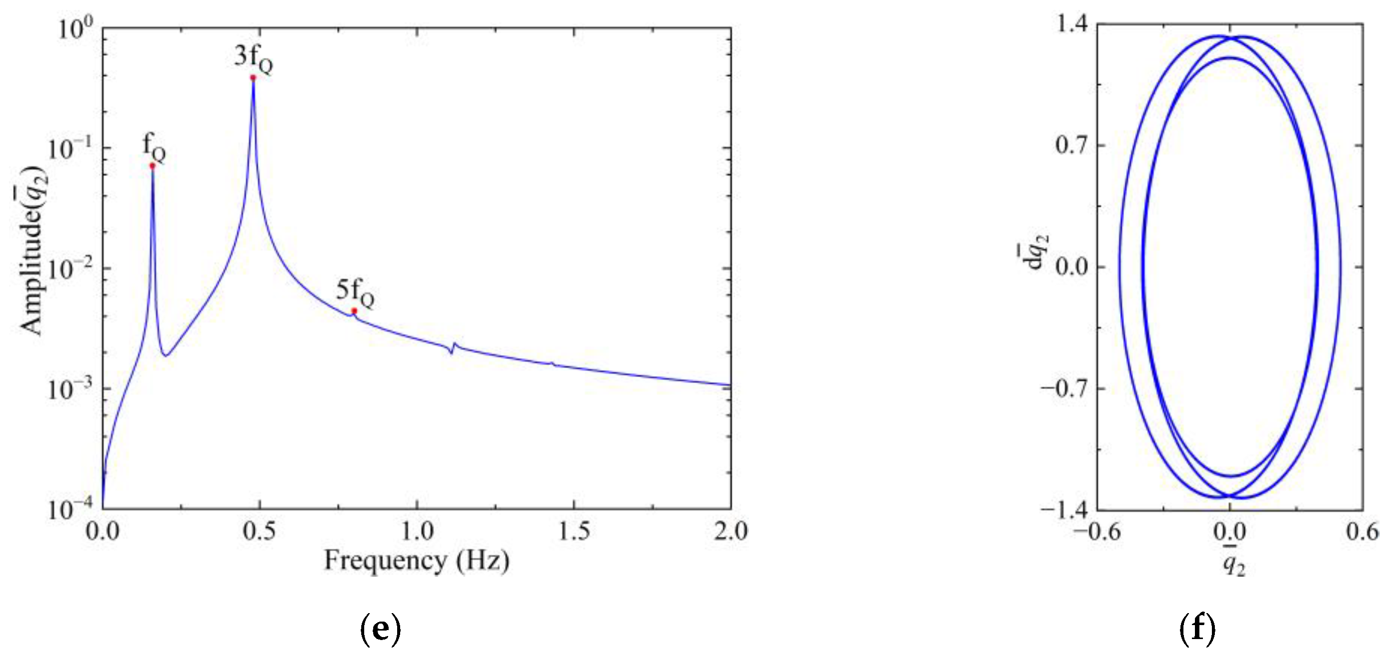
The steady responses of the blade with 40.28° and 44.81° are shown in Figure 8 and Figure 9, respectively. and are identified as periodic-1 motion and periodic-3 motion, respectively, and both and are governed by and its odd-fold multiples (i.e., , and so forth). The exchanges in energy between the modes can be observed clearly in Figure 8 but not in Figure 9. This is explained by the fact that the primary resonance is subjected to a strong enhancement on the steady response, which happens when 44.81°. Although the amplitude increases under primary resonance, the change in motion caused solely by internal resonance is minor and thus can hardly be observed in Figure 9.
The steady response of the blade when 85.48° is shown in Figure 10. Both and are found to be quasi-periodic with dominant spectra of , the first flapwise frequency and the combined frequencies of , and . With the current section of α, the aforementioned exchanges in energy between the aforementioned modes cannot be observed. In fact, the frequency difference between these modes grows with the increasing α (c.f. Figure 6b), which weakens the effect of internal resonance on these modes.
4.1.2. Effect of Contact Stiffness
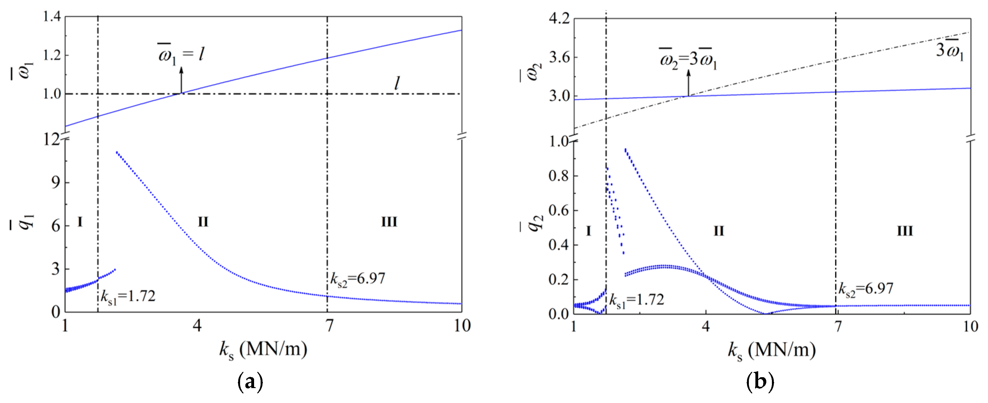
In the following, the vibration response of the blade is studied using different stiffness values of normal contact. The bifurcation of the blade vibration is shown in Figure 11, where the contact stiffness ranges from 1 MN/m to 10 MN/m. Similar to Section 4.1.1, the range of is divided into three stages, where and MN/m are the dividing points of these stages.
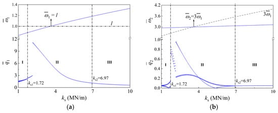
Figure 11.
Bifurcation of the blade with variable . (a) and (b) .
In Figure 11a, the steady is identified as a periodic-1 motion in the entire range of . Again, jumping of amplitude and hardening spring due to the primary resonance can be observed in stage-II. As for the steady second flapwise mode , it is periodic-1 in stages-I and III but periodic-3 in stage-II, Figure 11b. Moreover, the energy exchanges caused by internal resonance occur in stage-II; thereby, the jumping of the amplitude and the hardening spring due to the primary resonance can also be observed.
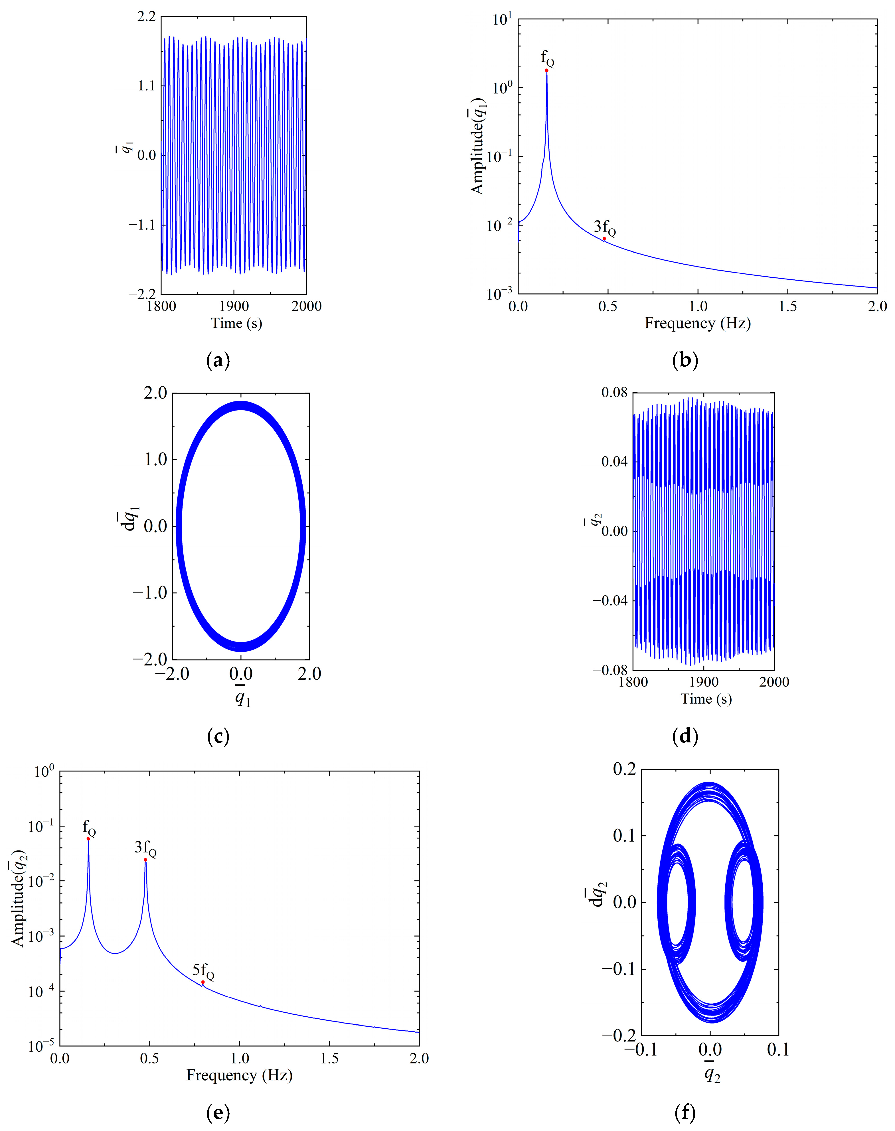
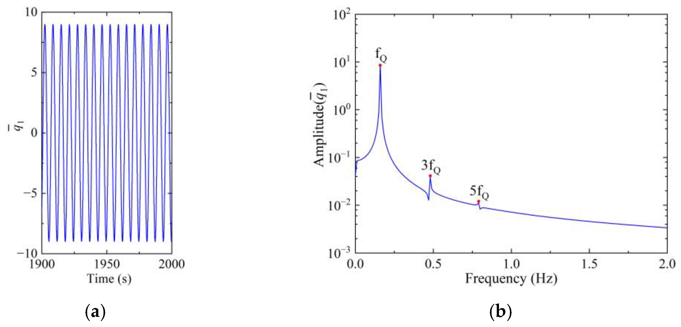
Further explorations are carried out using three different contact stiffness values, i.e., 1.407 MN/m (in stage-I), 2.764 MN/m (in stage-II) and 8.191 MN/m (in stage-III), and the response is provided through Figure 12, Figure 13 and Figure 14. As depicted in Figure 12, both and are periodic-1 motions and are spectrally governed by and its odd multiples ( and , etc.). Similar to previous cases, the amplitudes of and are both periodic, while the amplitude of is synchronous and π is out-of-phase against the amplitude of . Comparing the results presented in the three figures, it is found that the first flapwise modal response is always period-1. Nonetheless, the response of the second flapwise mode changes from a period-1 to period-3 motion and then returns to period-1 when the stiffness of normal contact increases.

Figure 12.
Steady responses of the blade with ks = 1.407 MN/m. (a) Time history, (b) frequency spectra and (c) phase diagram of ; (d) time history (e) frequency spectra and (f) phase diagram of .
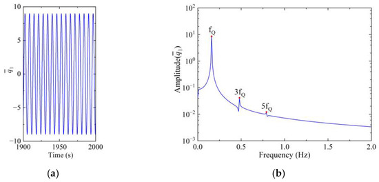
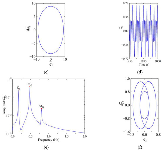
Figure 13.
Steady responses of the blade with ks = 2.764 MN/m. (a) Time history, (b) frequency spectra and (c) phase diagram of ; (d) time history, (e) frequency spectra and (f) phase diagram of .

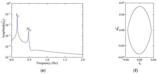
Figure 14.
Steady responses of the blade with ks = 8.191 MN/m. (a) Time history, (b) frequency spectra and (c) phase diagram of ; (d) time history, (e) frequency spectra and (f) phase diagram of .
4.1.3. The Effect of Rotation Speed
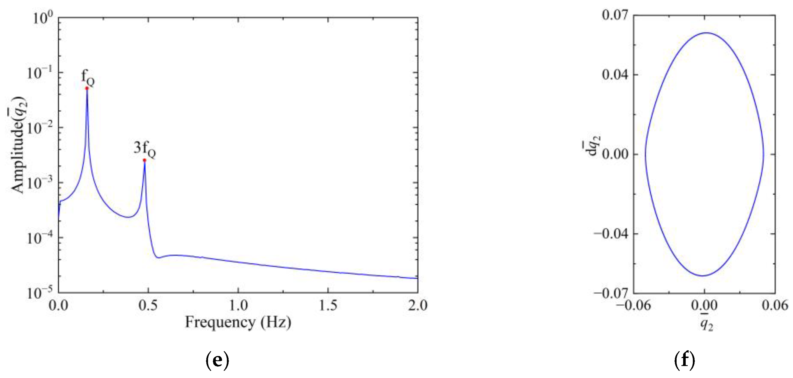
In the following, the contribution of the rotation speed to the blade vibration is studied. The bifurcation of the modal responses is shown in Figure 15, where the range of is from 2000 r/min to 12,000 r/min. This range of speed can also be divided into three stages: (stage-I), (stage-II) and r/min (stage-III), respectively, where 4.46 × 10³ r/min and 8.08 × 10³ r/min.
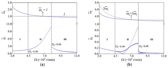
Figure 15.
Bifurcation diagram of the blade under variable W. (a) and (b) .
As shown in Figure 15a, the steady responses of remains in a periodic-3 motion for the entire range of . Similar to the case of contact stiffness, remains periodic-1 in stages-I and III, while is periodic-3 in stage-II, Figure 15b. Moreover, the jumping of the amplitude and the hardening spring can also be observed in stage-II due to the combination resonance.
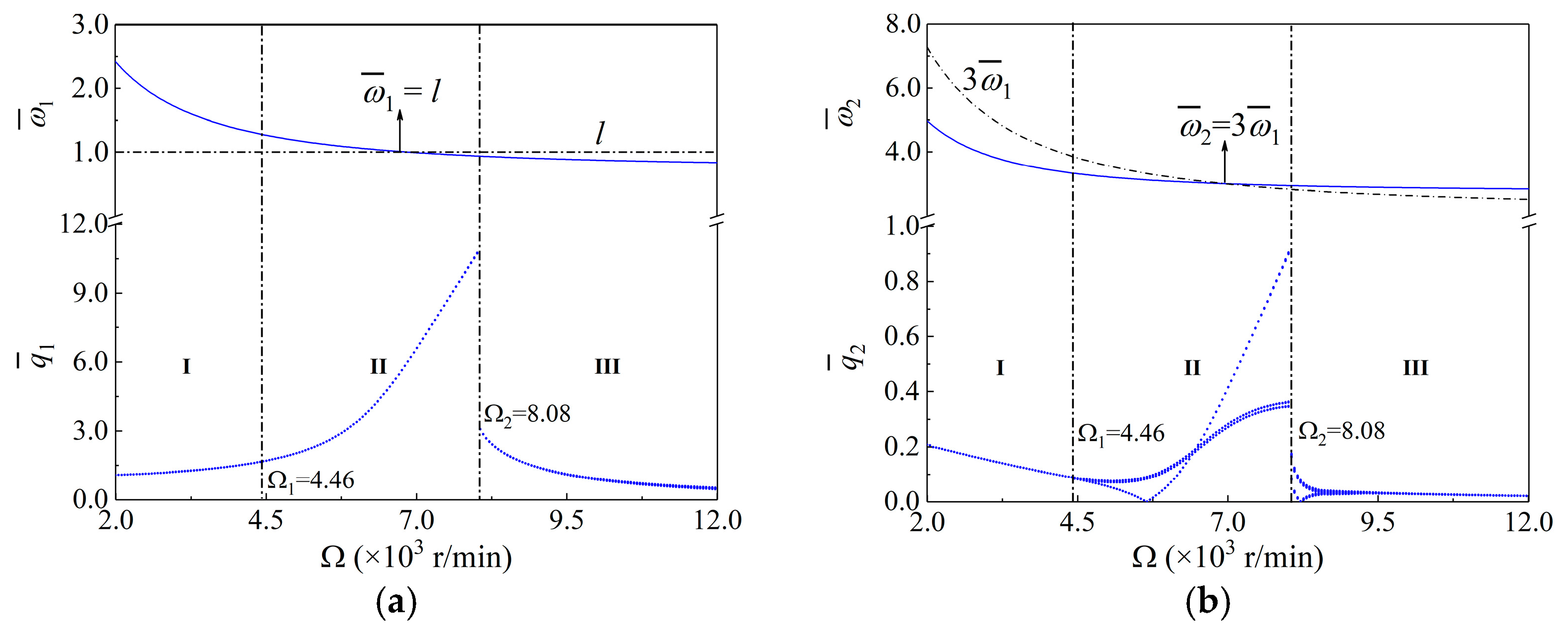
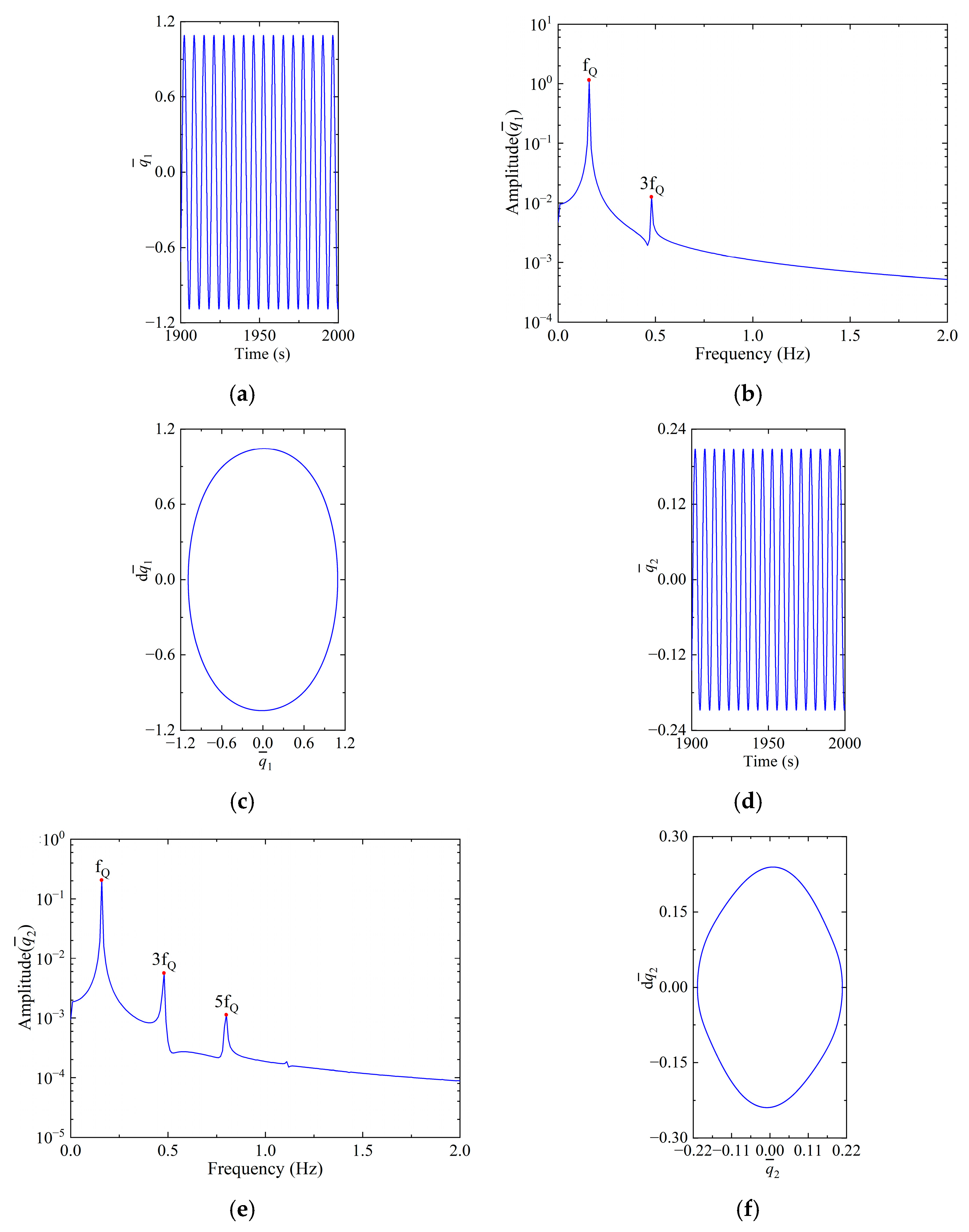
Next, three values of rotational speed, i.e., 2000 r/min (in stage-I), 7480 r/min (in stage-II) and 11,000 r/min (in stage-III), are chosen to examine the modal responses, Figure 16, Figure 17 and Figure 18. It is found that the steady first flapwise response is always period-1. However, the second flapwise modal response turns from the period-1 to period-3 motion and then goes back to period-1 with the increasing rotation speed. In addition, exchanges in energy can also be observed in stage-III, a sign of the interaction between modes of the first-order and second-order flapwise motion due to internal resonance.

Figure 16.
Steady responses with Ω = 2000 r/min. (a) Time history, (b) frequency spectra and (c) phase diagram of ; (d) time history, (e) frequency spectra and (f) phase diagram of .
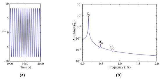
Figure 17.
Steady responses with Ω = 7480 r/min. (a) Time history, (b) frequency spectra and (c) phase diagram of ; (d) time history, (e) frequency spectra and (f) phase diagram of .
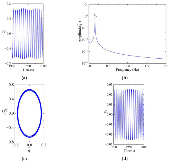
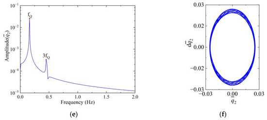
Figure 18.
Steady responses with Ω = 11,000 r/min. (a) Time history, (b) frequency spectra and (c) phase diagram of ; (d) time history, (e) frequency spectra and (f) phase diagram of .
4.2. Parametric Analysis in the Case of Combination Resonance
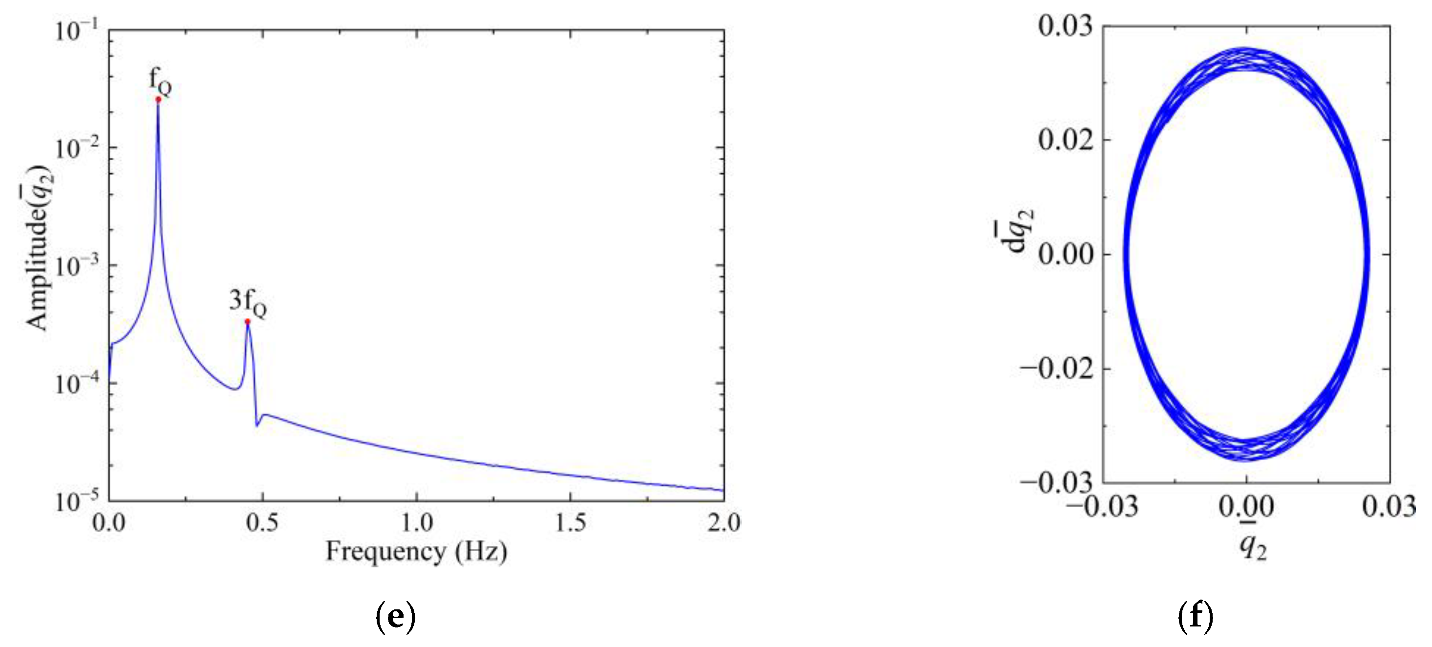
Based on Section 4.1, both primary and internal resonances can be observed in the steady responses of the first-order and second-order modes in the flapwise motion under variable tilting angle of the shroud, stiffness of normal contact and rotation speed. Also, combination resonance can be identified with the parameters in Table 1. In this section, the parametric influences of detuning and shroud design () are highlighted on the blade response in the case of combination resonance. It is worth noting that the forcing and damping parameters (i.e., and ) as well as the geometric nonlinearity coefficients are all related to and . For convenience, a coefficient of damping is defined for the flapwise modes of interest:
Based on Figure 19, for a fixed , the flapwise damping ratios rise as increases. Both decrease with the increasing when is constant. Further, the effect of on the modal dampings of the flapwise motion is noticeably weak compared with that of . In addition, the coefficient of the nondimensional equations in Appendix A shows that ascends as increases in contrast to . Both and are insensitive to the contact stiffness.

Figure 19.
Damping ratio of the first and second modes versus and . (a) and (b) . The colors represent the magnitudes of and .
4.2.1. Effect of with Various Contact Stiffness and Gap Dimension
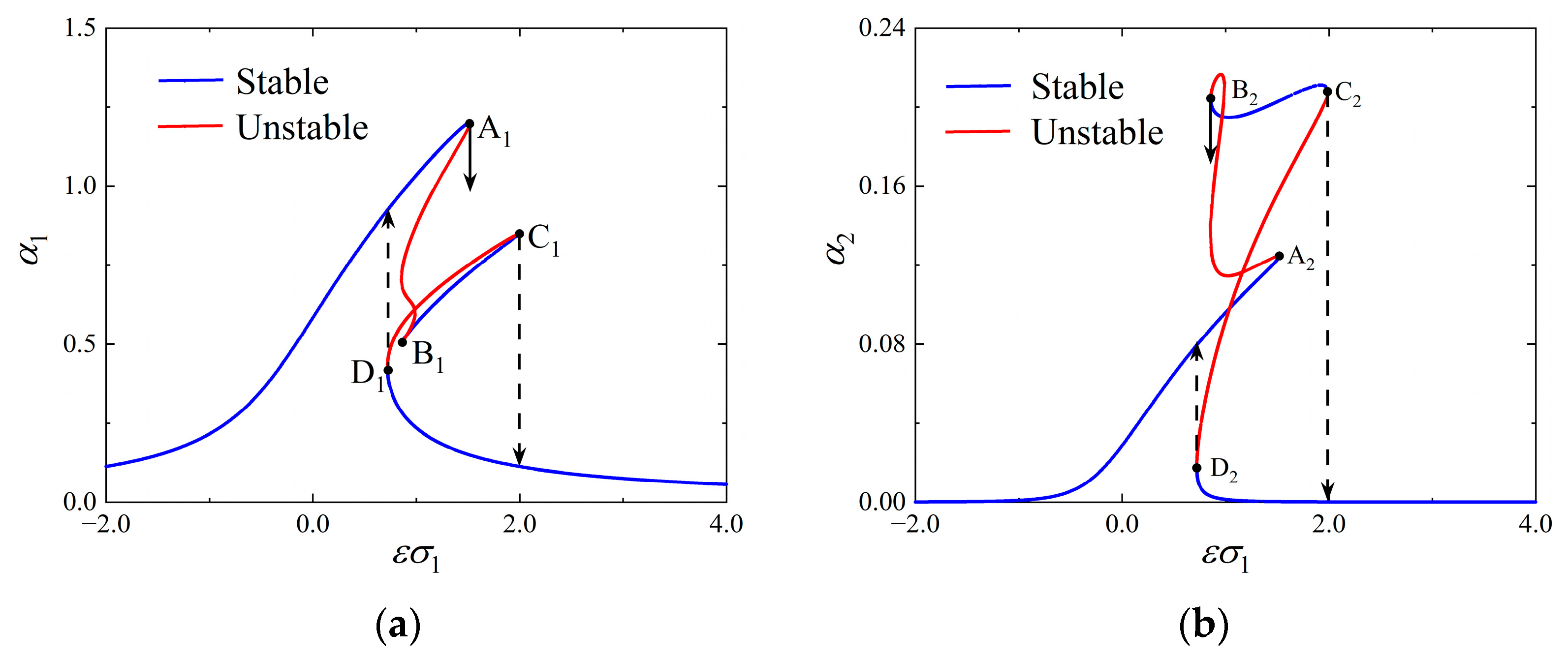
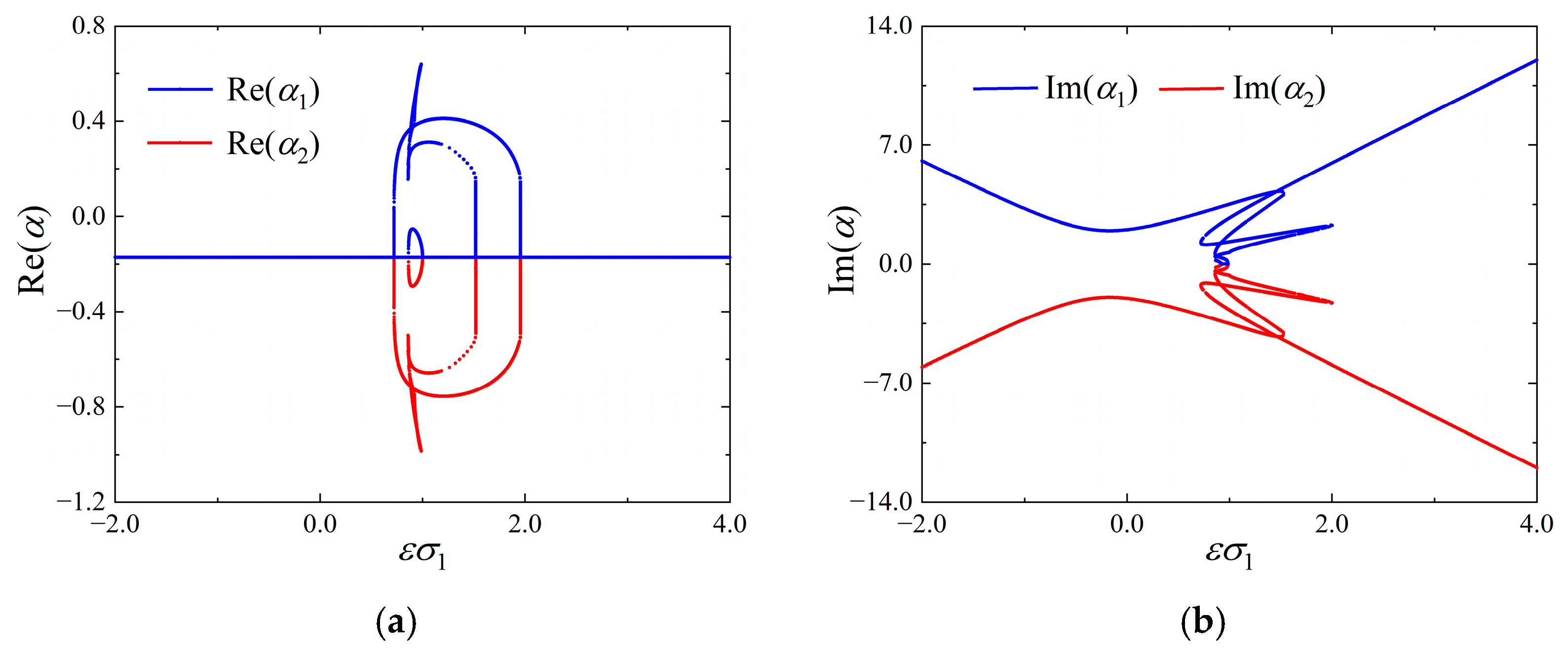
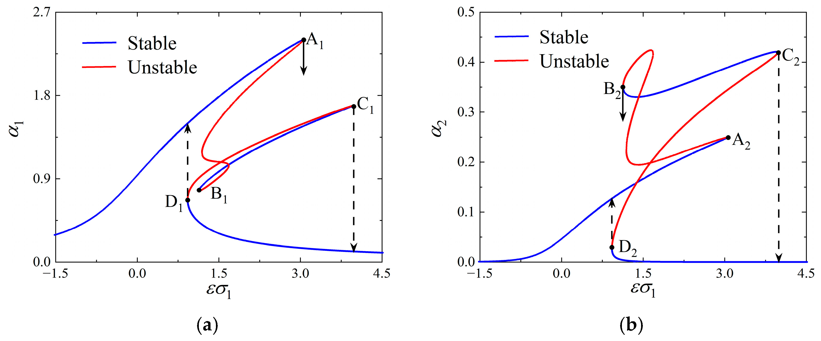
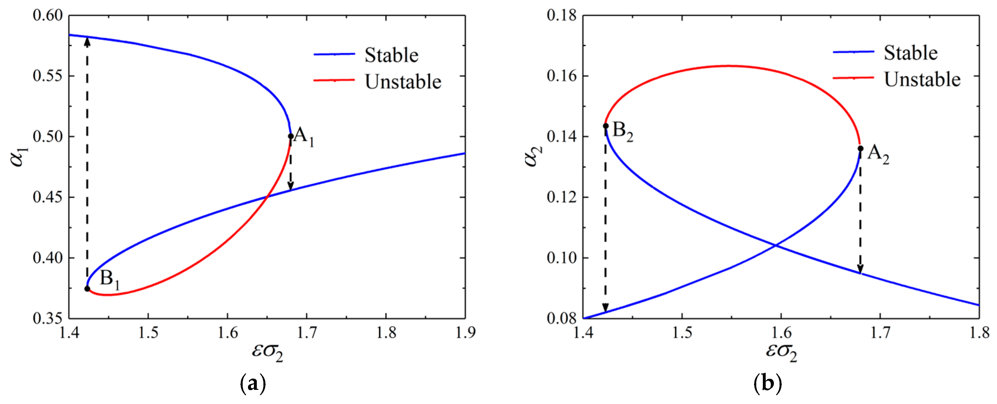
The amplitude–frequency relations of both and are presented in Figure 20 using different and constant = 3.55 × 10⁶ N/m and = 2 × 10⁻⁵ m for the case of combination resonance. It is observed that the blade resembles a hardened spring in vibration, which can be attributed to the presence of the terms. Based on Figure 20a, both stable and unstable motions can be identified within different bands of frequency, along with four turning points, i.e., A1, B1, C1 and D1. The real and imaginary parts of eigenvalues are presented in Figure 21, corresponding to the steady responses depicted in Figure 20.
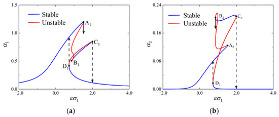
Figure 20.
Effect of in the case of combination resonance. (a) and (b) .
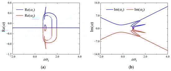
Figure 21.
Effect of on stability. (a) First flapwise mode and (b) second flapwise mode.
As far as the fixed points are concerned, the branch left to summit A1 () are stable focuses of before the occurrence of primary resonance. The connecting route from A1 to B1 () involves identified saddle-typed fixed points that destabilize . The branch between points B1 and C1 () has stable focuses at , as opposed to the saddle points represented by the branch from point C1 to D1 (). Moreover, the branch right of the turning point D1 returns to a stable focus. As a matter of fact, jumps downward from A1 and C1 once increases to critical values. The upward jumping happens at D1 as decreases to a certain critical value. However, with the decreasing , will jump at the turning point B1. The responses either jumps up and flows following the left branch of point A1 or goes down to the right branch of point D1.
As for in the case of combination resonance, a similar phenomenon of hardening can be observed in Figure 20b through three stable regions, two unstable regions and four turning points. Comparing the amplitudes in Figure 20a,b, the branches of response between points B2 () and C2 () are greater than that at A2 (), which makes a difference in the direction of jumping at points A2 () and B2 (); however, in the branch B1 () and C1 () are less than that at A1 (). This confirms the existence of energy exchange between the first and second modes in the flapwise direction.
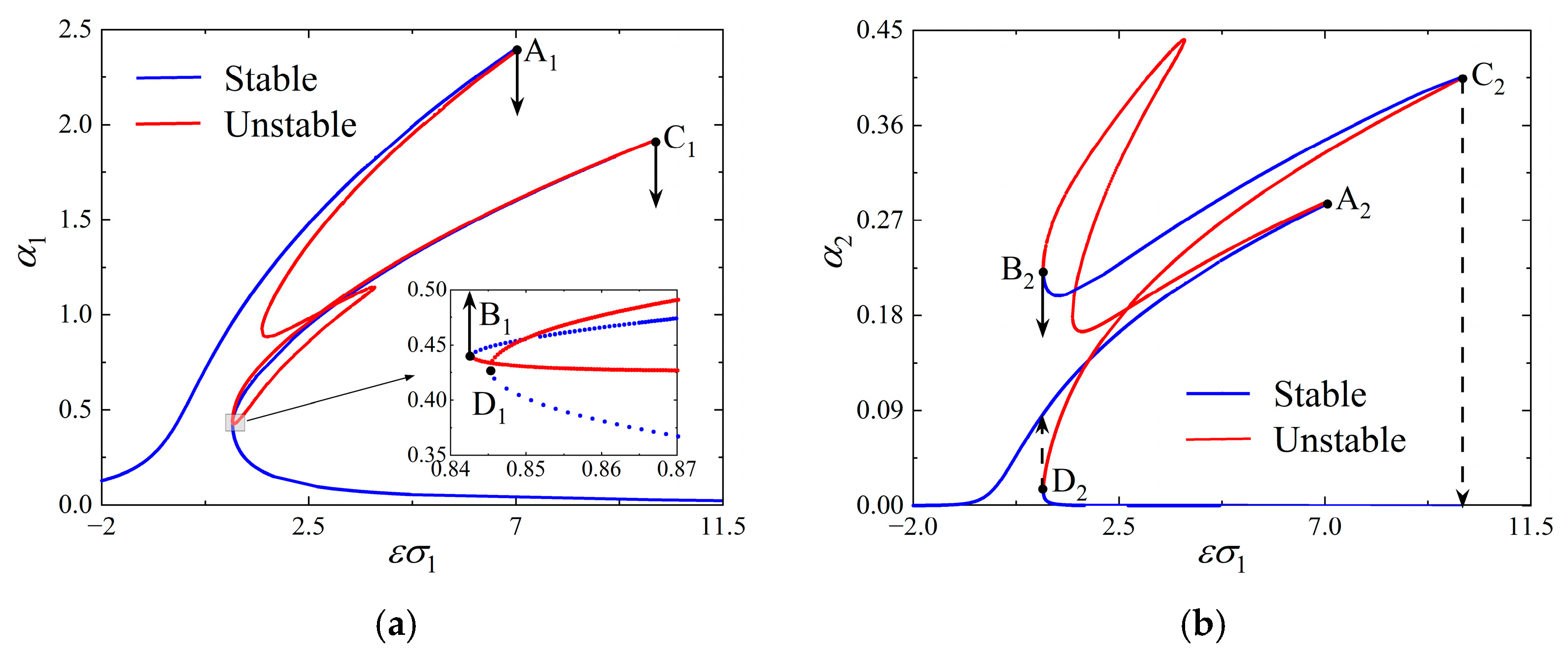
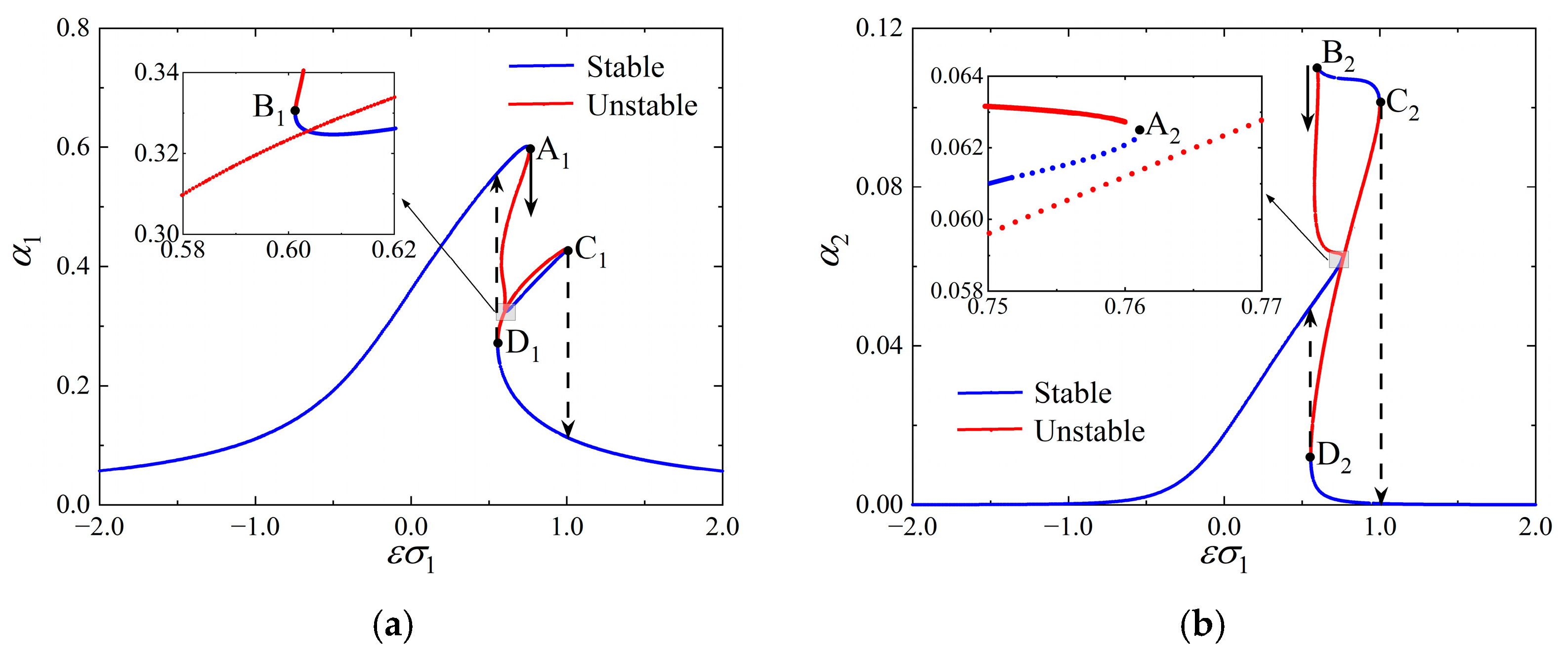
To demonstrate the effect of contact stiffness, is reduced by half (denoted subsequently by ) and doubled (by ), respectively. The solutions of and are presented in Figure 22 and Figure 23, respectively. Unlike the results shown in Figure 20, the decreasing widens the range of frequency corresponding to instability of the vibration and delays the onset frequency for primary resonance. Specifically, the frequency interval for unstable motion expands from (0.88, 1.52) and (0.72, 2.00) to (0.84, 7.05) and (0.83, 10.01), respectively. The larger is able to remove the instability of and under the combination resonance alongside the turning points. This is because the damping of the blade rises with the increasing (see Figure 19) and thus refrains the vibration of the blade. When is large enough, the hardening spring-like reaction of the blade at the resonance point can been completely suppressed.
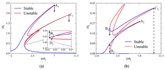
Figure 22.
Effect of in the case of combination resonance with . (a) and (b) .
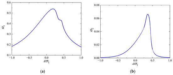
Figure 23.
Effect of in the case of combination resonance with a contact stiffness. (a) and (b) .
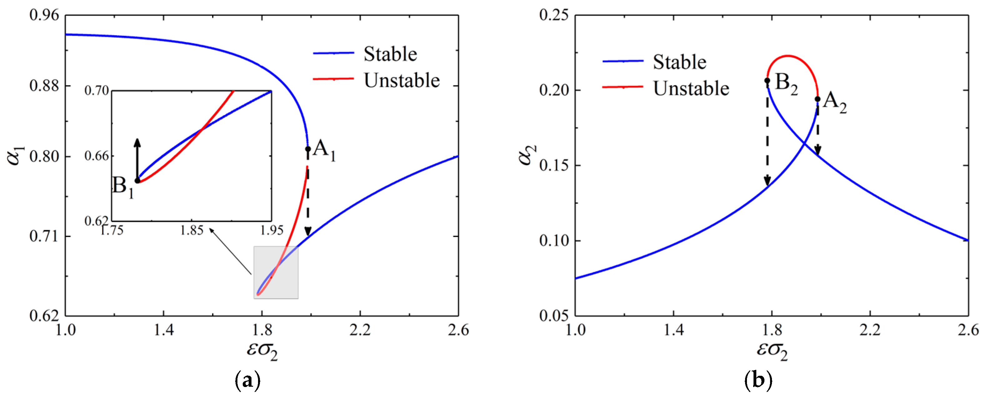
To demonstrate the effect of the shroud gap, the original is halved (denoted by ) and doubled (by ), respectively. The solutions of and are presented in Figure 24 and Figure 25, accordingly. Similar to the previous finding, the blade vibrates in higher amplitude as becomes larger, and the onset of primary resonance postpones. In this case, the regions of corresponding to instability expand from (0.88, 1.52) and (0.72, 2.00) to (1.14, 3.05) and (0.93, 3.97) and narrow to (0.60, 0.76) and (0.60, 0.76) in Figure 25 when the gap doubles its original value.
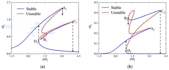
Figure 24.
Effect of in the case of combination resonance with a shroud gap. (a) and (b) .
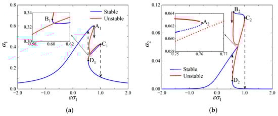
Figure 25.
Effect of in the case of combination resonance with a shroud gap. (a) and (b) .
Nevertheless, the effect of is noticeably weaker than that of . The rising influences the level of vibration through changing the aerodynamic force (), damping () and geometric nonlinear terms (). It is worth mentioning that changing has negligible contribution to the level of vibration [32,33]. An increasing has a double effect on the response: it does reduce the blade damping (see Figure 19) and hence increases the amplitudes of and ; on the other hand, it prevents the response by decreasing the aerodynamic force. Comparing Figure 24 with Figure 25, it is found that the level of vibration decreases with the increasing ; thereby, the strengthening of increasing on the level of vibration overwhelms its weakening.
4.2.2. Effect of with Various Contact Stiffness and Gap Dimension
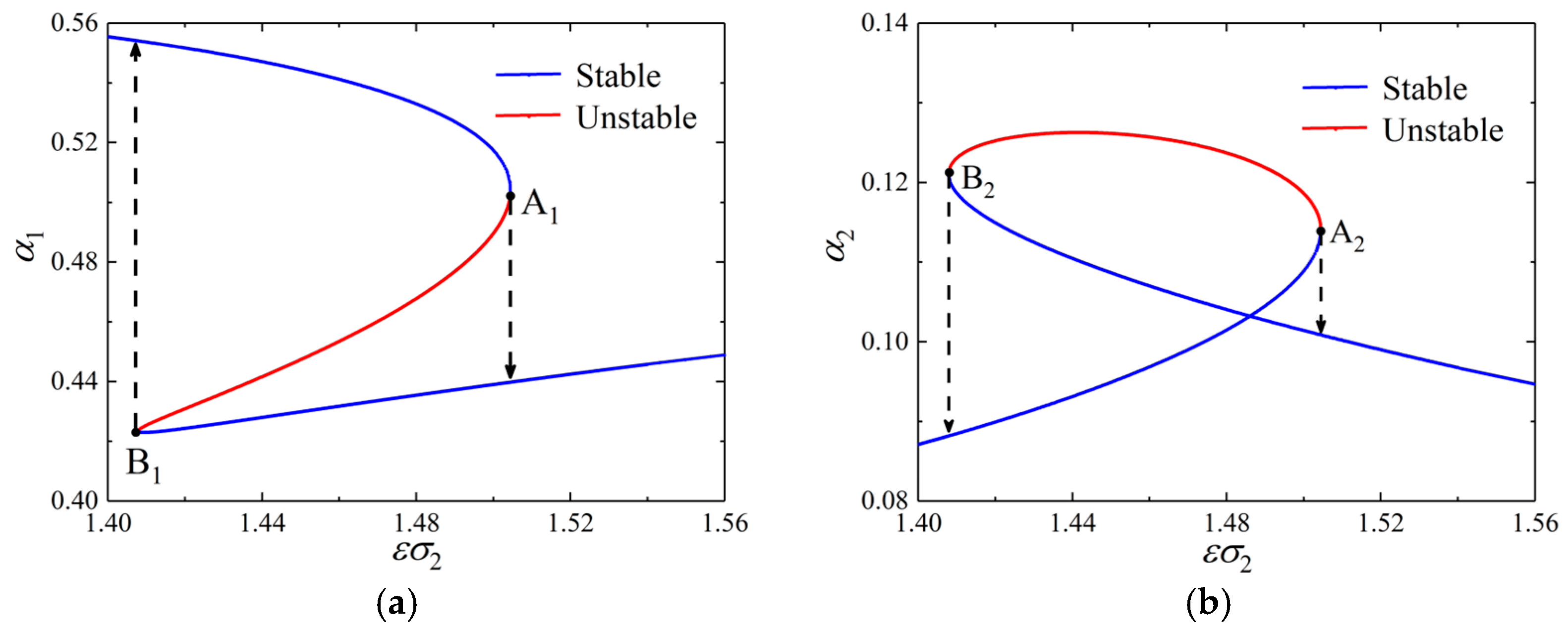
In this subsection, the contribution of parameter to the steady response of the blade is investigated. Given = 3.55 × 10⁶ N/m and = 2.0 × 10⁻⁵ m, the amplitudes of the first- and second-order modal response of the flapwise motion are plotted in Figure 26. Unlike the previous discussion, the phenomenon of softening spring are discovered due to the geometric nonlinearity associated with .
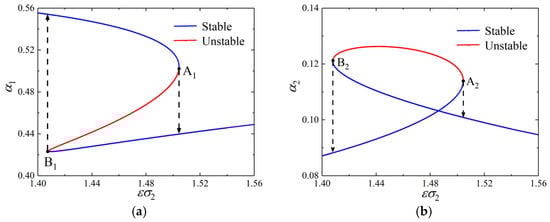
Figure 26.
Effect of in the case of combination resonance. (a) and (b) .
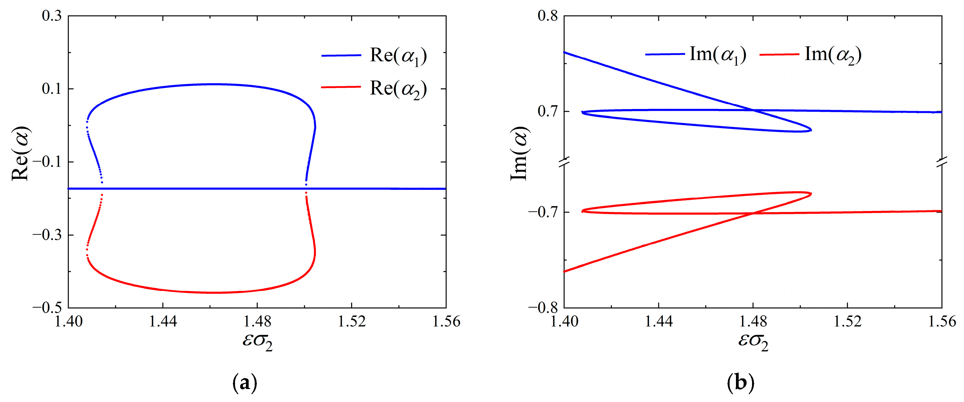
There are two regions of stable motion and one region of unstable motion along with two turning points, i.e., A1 and B1, as depicted in Figure 26a. The stability of the steady response is demonstrated through eigenvalue analysis at the fixed points of and in Figure 27. In viewing the fixed points, the branch left of point A1 () is found to be a stable focus of . The connection between A1 and the lowest point B1 () corresponds to the saddle points of , demonstrating an unstable motion of the blade. Indeed, jumps downward from point A1 once increases to be critical, while an upward jumping is located at point B1. As shown in Figure 26b, the hardening spring phenomenon can be observed alongside two stable regions and one unstable region. With the increasing , rises in the branch left of the turning point A2 and drops to the region left of the other turning point B2, which is opposite to the trend of in Figure 26a. This suggests that is the key influence on the internal resonance.
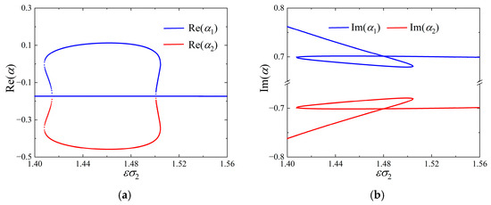
Figure 27.
Effect of on stability . (a) The first and (b) second flapwise modes.
The steady responses of the blade vibration versus are presented in Figure 28 and Figure 29 for the combination resonance. As shown in Figure 28, both the level of vibration and the interval of frequency for unstable motion are enlarged. There exists an overlap in the unstable region and the right branch of the turning point B1. The unstable region expands from (1.408, 1.504) to (1.423, 1.679). Similar to the solutions in Figure 23, the unstable region as well as the turning points can be removed by increasing for the same reason presented in Section 4.2.1.

Figure 28.
Effect of in the case of combination resonance with contact stiffness. (a) and (b) .
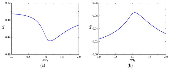
Figure 29.
Effect of in the case of combination resonance with contact stiffness. (a) and (b) .
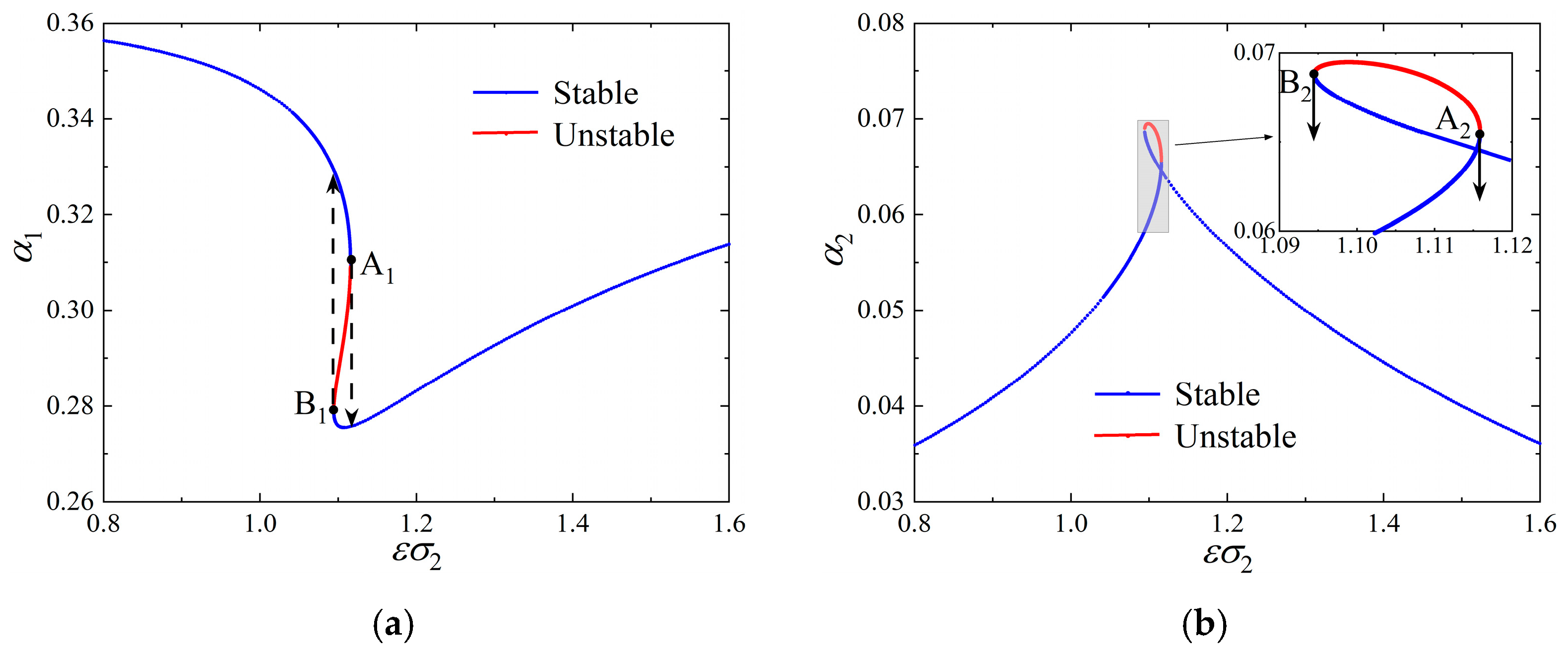
Finally, the steady responses in the situation of combination resonance are presented in Figure 30 and Figure 31 with various shroud gap . It is found that a decreasing escalates the vibration level and broadens the interval of instability of motion in the frequency domain. The unstable region now expands from (1.408, 1.504) to (1.783, 1.986) in the frequency domain at a halved and narrows to (1.097, 1.116) in Figure 31. The effect of on the responses is significantly weaker than that of on . In addition, the overlap in the unstable region and the right branch of the turning point B1 can also be observed in Figure 30a.

Figure 30.
Effect of in the case of combination resonance with a shroud gap. (a) and (b) .
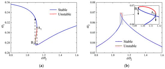
Figure 31.
Effect of in the case of combination resonance with a shroud gap. (a) and (b) .
5. Conclusions
In this paper, the nonlinear dynamics of a flexible turbine blade are investigated considering the contact and friction of shrouds, focusing on the case of combination resonance of flapwise motion induced by a 1:3 internal resonance between the first- and second-order modes and a primary resonance of the first-order mode. The stiffness and damping properties are expressed by linearizing the normal and tangential forces of shrouds using the method of harmonic balance. The steady responses of the blade in the situation of combination resonance are obtained with the multiple-scale method. The contributions of detuning and shroud parameters to the steady responses of the blade in the case combination resonance are analyzed. Several conclusions are drawn as follows:
- (1)
- The combination resonance involving the flapwise modes can be triggered by co-existing internal and primary resonances. Nevertheless, such resonance will not likely occur for separated blades where contact and friction on their shroud interfaces are removed.
- (2)
- Motion of the first-order flapwise mode can change from quasi-periodic to period-1 and then back to quasi-periodic with an increasing tilting angle of shroud. As for the second-order mode, it can change from quasi-periodic to period-3 and finally quasi-periodic.
- (3)
- With increasing contact stiffness and rotation speed, the first-order flapwise motion is period-1, while the second modal response can change between period-1 and period-1.
- (4)
- For primary resonance, the hardening spring behavior of the blade is attributed to geometric nonlinearity in the blade motion. On the other hand, such a nonlinearity can lead to a softening spring behavior of the blade in the scenario of internal resonance.
- (5)
- Less shroud contact stiffness and gap dimension can result in a stronger vibration response, wider region of unstable motion in the frequency domain and delayed onset of combination resonance.
Author Contributions
Conceptualization, H.L. and Y.W.; methodology, G.Y. and Y.W.; validation, H.L. and Y.W.; formal analysis, G.Y.; investigation, H.L. and Y.W.; resources, D.M. and Z.Y.; writing—original draft preparation, H.L. and G.Y.; writing—review and editing, Y.W.; funding acquisition, Y.W. and D.M. All authors have read and agreed to the published version of the manuscript.
Funding
The International Cooperation Fund Project of DBJI, Dalian University of Technology (ICR2109); the Free Exploration Project of the State Key Laboratory of Structural Analysis, Optimization and CAE Software for Industrial Equipment; and the National Science and Technology Major Project (2019-IV-0019-0087).
Data Availability Statement
The data presented in this study are available on request from the corresponding author. The data are not publicly available to protect the information of key design parameters.
Acknowledgments
The authors are grateful to DBJI (the Joint Institute of Dalian University of Technology and Belarus State University) and the State Key Laboratory of Structural Analysis, Optimization and CAE Software for Industrial Equipment for their sponsorships.
Conflicts of Interest
The authors declare no conflicts of interest. The funders had no role in the design of the study; in the collection, analyses, or interpretation of data; in the writing of the manuscript; or in the decision to publish the results. The authors declare that there are not any potential commercial interests.
Appendix A
The coefficients , , and of Equation (16) are defined as
where
The coefficients , , and of Equation (18) are defined as
The components of J in Equation (32) are defined as
Appendix B
An iterative can be applied to solve the amplitude of the steady vibration responses (i.e., B in Equation (2)) before the governing equations in the paper are solved. Let the initial value of B be denoted as B0. The properties of stiffness and damping can be determined by substituting B0 into Equations (8), (9), (11) and (12), which represented as , , and , respectively. Then, the steady responses of Equation (18) along with the transient systems (28)–(31) are solved using , , and , and the amplitude of the steady response is denoted by B1. The above process is repeated with B1 as the initial value until the error between Bi and Bi−1 is below the preassigned tolerance. At last, Bi is accepted as the amplitude of the desired steady responses.
References
- Cigeroglu, E. Development of Microslip Friction Models and Forced Response Prediction Methods for Frictionally Constrained Turbine Blades. Ph.D. Thesis, The Ohio State University, Columbus, OH, USA, 2007. [Google Scholar]
- Xie, F.; Ma, H.; Cui, C.; Wen, B. Vibration response comparison of twisted shrouded blades using different impact models. J. Sound Vib. 2017, 397, 171–191. [Google Scholar] [CrossRef]
- Ju, D.; Sun, Q. Modeling of a Wind Turbine Rotor Blade System. J. Vib. Acoust. 2017, 139, 051013. [Google Scholar] [CrossRef]
- Chiu, Y.J.; Chen, D.Z.; Yang, C.H. Influence on Coupling Vibration of Rotor System with Grouped Blades due to Mistuned Lacing Wire. Appl. Mech. Mater. 2011, 101–102, 1119–1125. [Google Scholar] [CrossRef]
- Ma, H.; Xie, F.; Nai, H.; Wen, B. Vibration characteristics analysis of rotating shrouded blades with impacts. J. Sound Vib. 2016, 378, 92–108. [Google Scholar] [CrossRef]
- Chatterjee, A.; Kotambkar, M.S. Modal characteristics of turbine blade packets under lacing wire damage induced mistuning. J. Sound Vib. 2015, 343, 49–70. [Google Scholar] [CrossRef]
- Shadmani, M.; Tikani, R.; Ziaei-Rad, S. On using a distributed-parameter model for modal analysis of a mistuned bladed disk rotor and extracting the statistical properties of its in-plane natural frequencies. J. Sound Vib. 2019, 438, 324–343. [Google Scholar] [CrossRef]
- Zhou, X.; Huang, K.; Li, Z. Geometrically nonlinear beam analysis of composite wind turbine blades based on quadrature element method. Int. J. Non-Linear Mech. 2018, 104, 87–99. [Google Scholar] [CrossRef]
- Karimi, A.H.; Shadmani, M. Nonlinear vibration analysis of a beam subjected to a random axial force. Arch. Appl. Mech. 2019, 89, 385–402. [Google Scholar] [CrossRef]
- Griffin, J.H. Friction Damping of Resonant Stresses in Gas Turbine Engine Airfoils. J. Eng. Power 1980, 102, 329–333. [Google Scholar] [CrossRef]
- Menq, C.-H.; Bielak, J.; Griffin, J. The influence of microslip on vibratory response, part I: A new microslip model. J. Sound Vib. 1986, 107, 279–293. [Google Scholar] [CrossRef]
- Iwan, W.D. On a Class of Models for the Yielding Behavior of Continuous and Composite Systems. J. Appl. Mech. 1967, 34, 612–617. [Google Scholar] [CrossRef]
- Yang, B.; Menq, C. Characterization of 3D contact kinematics and prediction of resonant response of structures having 3D frictional constraint. J. Sound Vib. 1998, 217, 909–925. [Google Scholar] [CrossRef]
- Nan, G.; Lou, J.; Song, C.; Tang, M. A New Approach for Solving Rub-Impact Dynamic Characteristics of Shrouded Blades Based on Macroslip Friction Model. Shock. Vib. 2020, 2020, 8147143. [Google Scholar] [CrossRef]
- Brach, R.M. Mechanical Impact Dynamics: Rigid Body Collisions; John Wiley & Sons: New York, NY, USA, 1991. [Google Scholar]
- He, B.; Ouyang, H.; He, S.; Ren, X.; Mei, Y. Dynamic analysis of integrally shrouded group blades with rubbing and impact. Nonlinear Dyn. 2018, 92, 2159–2175. [Google Scholar] [CrossRef]
- He, S.; Si, K.; He, B.; Yang, Z.; Wang, Y. Rub-Impact Dynamics of Shrouded Blades under Bending-Torsion Coupling Vibration. Symmetry 2021, 13, 1073. [Google Scholar] [CrossRef]
- Mashayekhi, F.; Nobari, A.; Zucca, S. Hybrid reduction of mistuned bladed disks for nonlinear forced response analysis with dry friction. Int. J. Non-Linear Mech. 2019, 116, 73–84. [Google Scholar] [CrossRef]
- She, H.; Li, C.; Tang, Q.; Wen, B. Veering and merging analysis of nonlinear resonance frequencies of an assembly bladed disk system. J. Sound Vib. 2021, 493, 115818. [Google Scholar] [CrossRef]
- Wei, S.-T.; Pierre, C. Localization Phenomena in Mistuned Assemblies with Cyclic Symmetry Part II: Forced Vibrations. J. Vib. Acoust. 1988, 110, 439–449. [Google Scholar] [CrossRef]
- Fang, X.; Tang, J.; Jordan, E.; Murphy, K. Crack induced vibration localization in simplified bladed-disk structures. J. Sound Vib. 2006, 291, 395–418. [Google Scholar] [CrossRef]
- Picou, A.; Capiez-Lernout, E.; Soize, C.; Mbaye, M. Robust dynamic analysis of detuned-mistuned rotating bladed disks with geometric nonlinearities. Comput. Mech. 2020, 65, 711–730. [Google Scholar] [CrossRef]
- Zhao, W.; Zhang, D.; Xie, Y. Vibration analysis of mistuned damped blades with nonlinear friction and contact. J. Low Freq. Noise Vib. Act. Control. 2019, 38, 1505–1521. [Google Scholar] [CrossRef]
- Larsen, J.W.; Nielsen, S.R.K. Nonlinear parametric instability of wind turbine wings. J. Sound Vib. 2007, 299, 64–82. [Google Scholar] [CrossRef]
- Karimi, B.; Moradi, H. Nonlinear kinematics analysis and internal resonance of wind turbine blade with coupled flapwise and edgewise vibration modes. J. Sound Vib. 2018, 435, 390–408. [Google Scholar] [CrossRef]
- Zhang, W.; Liu, G.; Siriguleng, B. Saturation phenomena and nonlinear resonances of rotating pretwisted laminated composite blade under subsonic air flow excitation. J. Sound Vib. 2020, 478, 115353. [Google Scholar] [CrossRef]
- Chu, S.; Cao, D.; Sun, S.; Pan, J.; Wang, L. Impact vibration characteristics of a shrouded blade with asymmetric gaps under wake flow excitations. Nonlinear Dyn. 2013, 72, 539–554. [Google Scholar] [CrossRef]
- Allara, M. A model for the characterization of friction contacts in turbine blades. J. Sound Vib. 2009, 320, 527–544. [Google Scholar] [CrossRef]
- Pai, P.; Rommel, B.; Schulz, M.J. Non-linear vibration absorbers using higher order internal resonances. J. Sound Vib. 2000, 234, 799–817. [Google Scholar] [CrossRef]
- Sayed, M.; Kamel, M. 1:2 and 1:3 internal resonance active absorber for non-linear vibrating system. Appl. Math. Model. 2012, 36, 310–332. [Google Scholar] [CrossRef]
- Eftekhari, M.; Ziaei-Rad, S.; Mahzoon, M. Vibration suppression of a symmetrically cantilever composite beam using internal resonance under chordwise base excitation. Int. J. Non-Linear Mech. 2013, 48, 86–100. [Google Scholar] [CrossRef]
- Li, L.; Li, Y.; Liu, Q.; Lv, H. Flapwise non-linear dynamics of wind turbine blades with both external and internal resonances. Int. J. Non-linear Mech. 2014, 61, 1–14. [Google Scholar] [CrossRef]
- Yuan, G.; Wang, Y. Internal, primary and combination resonances of a wind turbine blade with coupled flapwise and edgewise motions. J. Sound Vib. 2021, 514, 116439. [Google Scholar] [CrossRef]
- She, H.; Li, C. Effects of centrifugal stiffening and spin softening on nonlinear modal characteristics of cyclic blades with impact–friction coupling. Nonlinear Dyn. 2022, 110, 3229–3254. [Google Scholar] [CrossRef]
- Nayfeh, A.H.; Mook, D.T. Nonlinear Oscillations; John Wiley & Sons: New York, NY, USA, 1995. [Google Scholar]


Disclaimer/Publisher’s Note: The statements, opinions and data contained in all publications are solely those of the individual author(s) and contributor(s) and not of MDPI and/or the editor(s). MDPI and/or the editor(s) disclaim responsibility for any injury to people or property resulting from any ideas, methods, instructions or products referred to in the content. |
© 2024 by the authors. Licensee MDPI, Basel, Switzerland. This article is an open access article distributed under the terms and conditions of the Creative Commons Attribution (CC BY) license (https://creativecommons.org/licenses/by/4.0/).