Abstract
The braking performance of hydrodynamic retarders is critical for the safety and economy of heavy-duty vehicles. In order to effectively improve the braking system to meet the needs of the market, an evaluation method for quantifying the performance of hydrodynamic retarders is imperative. In this paper, ten evaluation criteria are put forward according to relevant national standards and market requirements, then the scores corresponding to these criteria are obtained by performance bench test. A fuzzy modification of the analytic hierarchy process (AHP) method is applied to determine the relative weights of the chosen evaluation criteria, where uncertain and imprecise judgments of decision-makers are translated into fuzzy numbers. Furthermore, the improved radar chart method is used to comprehensively evaluate and rank the braking performance of three types of hydrodynamic retarders as an empirical example. In addition, the weight sensitivity analysis is conducted to examine the robustness of the ranking results. The results show that the proposed method is effective and feasible. It provides a reference for multi-objective optimization control strategies and structure designs of hydrodynamic retarders.
1. Introduction
Hydrodynamic retarders are required for heavy-duty vehicles during retarding or non-emergency braking conditions to slow down the vehicle or maintain a steady speed on long downgrades, and thus increases the life of the service brake [1]. In recent years, diverse hydrodynamic retarders have been produced to meet various market demands, and the improvement of the braking performance of hydrodynamic retarders is a growing concern. Not only is an effective integration into the vehicle braking system required for hydrodynamic retarders, but also the requirements for high braking torque, low unit weight, and good thermal decay characteristics. Therefore, it is difficult to quantitatively and qualitatively evaluate the overall braking performance of hydrodynamic retarders based on the complex criteria.
Many different theories of braking performance for conducting an evaluation have been proposed for many years. Yu Wang and Li Lin [2] evaluated the performance of pneumatic disc brakes, hydraulic disc brakes, and pneumatic band brakes in terms of braking capacity, response speed, braking efficiency, and control accuracy. Kwangki Jeon et al. [3] evaluated the fail-safe control strategies of brake-by-wire systems in various failure modes combined with a longitudinal deceleration deviation term and a lateral deviation term. Peirong Jia [4] analyzed the impact of engine brake power, cooling fan (on or off), and vehicle weight on vehicle downhill drivability at both sea level and high altitudes. However, it is not sufficient to evaluate the braking performance of hydrodynamic retarders only by using these traditional braking parameters. In addition, the performance evaluation criteria hierarchy of hydrodynamic retarders is rarely reported, and the evaluation method of hydrodynamic retarders needs to be further studied.
Choosing a suitable method for evaluating criteria aids evaluators and analysts in effectively assessing and determining the optimal alternative. When employing criteria to choose from a range of alternatives, it becomes crucial to consider conflicting factors [5]. For example, two criteria used to select a hydrodynamic retarder of good braking performance might be brake efficiency and brake temperature. These two criteria are in conflict with each other because an attempt to increase brake efficiency causes a rise in brake temperature. Hence, this problem should be solved by a multi-criteria method [6]. Multi-criteria decision-making involves a multi-stage process of (i) defining objectives, (ii) choosing the criteria to measure the objectives, (iii) specifying alternatives, (iv) assigning weights to the criteria, and (v) applying the appropriate mathematical algorithm for ranking alternatives [7].
Several methods have been proposed in the literature and have been utilized to address a range of MCDM issues [8]. The technique for order preference by similarity to ideal solution (TOPSIS) was developed by Hwang and Yoon in 1981 [9]. The key idea behind TOPSIS is to determine the optimal alternative by comparing each option against both the ideal and anti-ideal solutions. However, the methodology might not fully capture the complexities of uncertain environments. Cluster analysis is a powerful technique used in MCDM to group similar alternatives based on their characteristics or performance across multiple criteria. It is an unsupervised learning method that aims to identify natural groupings or clusters within a dataset without any predefined labels or target outcomes. It is essential to note that cluster analysis cannot provide explicit preference information or a ranking of alternatives. Artificial neural networks (ANNs), have shown promise and have been applied in MCDM as powerful tools for solving complex decision problems. It is important to note that the successful application of neural networks in MCDM often requires sufficient and relevant data. Analytic hierarchy process (AHP) is widely used for multi-criteria decision-making and has successfully been applied to braking performance decision-making problems [10]. Hendre, KN and Bachchhav, BD [11] applied AHP to evaluate the criticality property of a novel brake pad material. The main advantages of AHP are handling multiple criteria, being easy to understand, and being able to effectively handle both qualitative and quantitative data. However, factor comparisons often involve some amount of uncertainty and subjectivity. For example, experts may know one factor is more important than another, but they might not be able to provide a definite scale for the comparison due to uncertainty regarding the degree of importance. In this case, the classical AHP method has to be discarded due to the existence of fuzzy or incomplete comparisons. Among decision-making methodologies, the fuzzy analytic hierarchy process (FAHP), first introduced by Laarhoven and Pedrycz, is a powerful tool to treat uncertainty in the case of incomplete or vague information. FAHP takes into account the dependencies between criteria, helping to identify how changes in one criterion may impact others. This feature allows for a more holistic evaluation of the decision problem and helps in understanding the cause-and-effect relationships among criteria. It has been applied in various fields, including control engineering, artificial intelligence [12], management science [13], and multiple criteria decision making, among others.
However, the above method can not display evaluation results in a visual mode, the importance of each factor is not described clearly, and the resultant ordering is difficult for several objects with similar braking performance. The radar chart method is a multi-variable analytical method for comprehensive evaluation [14]. Not only the overall advantage of evaluation objects but also the coordinated development of all aspects can be considered so that it reflects the comprehensive strengths of the objects more completely [15]. The most distinct characteristic of the radar chart is that it can display the status of to-be-evaluated objects intuitively [16]. However, the shape of the radar chart is related to the order of the respective indices, resulting in non-unique evaluation results. Additionally, the angles of the radar chart, which represent the weights of the indices are equal, so it can not reflect the influence degree of the indices used to evaluate the given objects [17]. Therefore, this paper proposes an improved radar chart (IRC) that incorporates the weights and values of the indices to make a qualitative evaluation.
In this paper, a fuzzy analytic hierarchy process method based on improved radar chart is suggested to select the best hydrodynamic retarder. For this aim, three main criteria and ten sub-criteria are proposed for constructing a hierarchical structure of performance evaluation, and three types of hydrodynamic retarder alternatives are evaluated. Performance tests of three types of hydrodynamic retarders are carried out to obtain the evaluation value set of corresponding criteria. Then, the fuzzy analytic hierarchy is applied to calculate the weights of the evaluation criteria. The imprecise decision-maker’s judgments are represented as fuzzy numbers rather than exact numerical values. Furthermore, the improved radar chart is used to analyze the hydrodynamic retarder brake capabilities and to compare the braking performance of different types of hydrodynamic retarders. It further provides suggestions based on the research results for performance evaluation and serves as a reference for future research in this field.
The paper is structured as follows: Section 2 presents the related evaluation criteria and hierarchical structure model of the braking performance. In Section 3, the content and process of performance test are described. Then, the introduction to the fuzzy analytic hierarchy process is given in Section 4. Section 5 provides a comprehensive and visual evaluation method for ranking and selection of braking performance. Finally, the proposed method is illustrated with a case study of the three types of hydrodynamic retarders, and a sensitivity analysis of results is presented in Section 6. The main conclusions, limitations, and future works are summarized in Section 7.
2. Evaluation Criteria
The basic performance requirements of hydrodynamic retarders are good braking performance at low speeds, a quick response system, smooth braking torque, and good thermal decay performance [18]. To propose the criteria from multiple angles, a detailed literature search focusing on concepts related to braking performance evaluation was conducted. Additionally, this research collaborates with a team of experts with years of experience in their respective fields related to braking systems, including automotive engineering, mechanical engineering, vehicle dynamics, safety standards, and braking performance analysis.
Performance evaluation of hydrodynamic retarders is a multi-level and multi-factor comprehensive evaluation problem. In order to facilitate calculation and analysis, the evaluation criteria for this paper are divided into two levels: main criteria and sub-criteria. A good braking performance can improve brake capability and brake safety of hydrodynamic retarders, and reduce unnecessary costs. For this, the main criteria are designed, consisting of (1) Capability, which refers to the ability to stop quickly and efficiently, (2) Safety, which refers to the probability of avoiding accidents and mitigating the severity of collisions [19], and (3) Economy, which is related to service life and maintenance [20]. The definitions, industry standards, and influencing factors of the sub-criteria are briefly explained in the following:
- . Capability
- -
- . Maximum braking torque (N·m):In the hydrodynamic retarder, the rotor drives the transmission fluid to circulate in the working chamber so that braking torque is generated by a reaction force between the rotating blades and the stationary blades. When the hydrodynamic retarder is completely filled and operates at the rated rotational speed, the braking torque reaches its maximum value. The maximum braking torque represents the braking capacity of the hydrodynamic retarder. The braking torque can be calculated by the following equation [1]:where is the performance coefficient, is the oil density (kg/m3), g is the acceleration of gravity (m/s2), n is the rotational speed (rpm), D is the circular circle diameter (m).According to the formula, the maximum braking torque mainly depends on the density of the working medium and the structural parameters. Theoretically, the larger the density of the working medium, the larger the braking torque. In fact, considering that the working fluid, in addition to transferring power, also lubricates, cools, and cleans moving parts, the resistance of the fluid should not exceed a certain threshold, and the density of the working medium must be within a reasonable range [21]. The structural parameters of hydrodynamic retarders are the key factors affecting the maximum braking torque, including the blade parameters and the circular circle parameters. Blade parameters, such as blade number, blade lean angle [22], and blade leading angle, directly impact the internal flow field within the working chamber. In addition, the main parameter of the circle is the diameter, as shown in Figure 1. In the process of design optimization, it is necessary to consider all factors comprehensively in order to achieve the optimal braking capacity.
 Figure 1. Schematic diagram of blade structure of hydrodynamic retarder.
 - -
- . Maximum input rotational speed (rpm):In the drive train, the engine’s crankshaft drives a rotor located in the power flow, while the stator is fixed to the retarder housing. A hydrodynamic retarder is installed behind the gearbox. According to its arrangement with the drive shaft, it can be divided into in-line and off-line, as shown in Figure 2. In-line retarders are installed directly onto the transmission or freely to the driveline. They are connected to the universal joint shaft of the vehicle. On the other hand, off-line retarders work with a conversion ratio which means that the speed of the retarder is greater than that of the drive shaft . Off-line retarders are highly compact and exhibit great braking force even at low speeds. Meanwhile, the maximum input rotational speed is also based on the mechanical load.
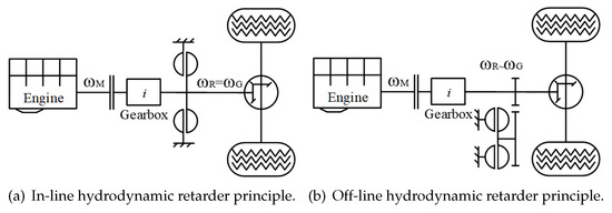 Figure 2. Alternative positions for mounting hydrodynamic retarder.
 - -
- . Braking pressure (MPa):When the brake pedal is pushed, it depresses a piston in the master cylinder, building up hydraulic pressure to open the valves that allow fluid to charge the working chamber of the hydrodynamic retarder. The pressure required to reach a specified braking torque is the braking pressure [23]. The braking pressure is an important criterion reflecting the stiffness and strength of the braking system. The braking pressure directly affects the response characteristic of the whole braking system and the pedal sensation of the driver. The relationship between pedal force and braking pressure is an important parameter. If excessive force is demanded from the driver on the brake pedal, it can result in fatigue and compromise the vehicle’s safe operation. Conversely, if excessive hydraulic pressure is generated by the master cylinder, the vehicle may come to a screeching stop.
- . Safety
- -
- . Brake action time (s):The brake action time refers to the duration it takes to achieve a specified level of braking once the braking process has been initiated [24]. This time should be sufficient to effectively slow down the vehicle and provide a safe and comfortable braking experience for the driver without causing abrupt stops for the passengers. Generally, the brake action time of the hydrodynamic retarder should be less than 1 s. Figure 3 divides the entire braking time into separable periods that are related to different actions of the hydrodynamic retarder. Hydrodynamic retarder is activated via the foot brake pedal or the hand lever on the steering wheel. A short brake action time can decrease braking distance. The brake action time is associated with the spool diameter of the control valve, fluid viscosity, the length of the hydraulic piping, and the control method. The larger the spool diameter, the shorter the time of the working chamber to reach the target filling rate. As fluid viscosity increases, the time required for fluid to fill through the piping increases due to the slower flow rate, resulting in the brake acting for a longer time [25]. In addition, if the hydrodynamic retarder is farther away from the control valve, the control signal will be further delayed.
 Figure 3. Braking time distribution of hydrodynamic retarder.
 - -
- . Stability for braking torque (%):One of the primary functions of the hydrodynamic retarder is to provide a desired constant braking torque for heavy-duty vehicles being driven downhill according to the driver’s intention. The operational accuracy of the braking torque represents the braking stability and smoothness of the resulting deceleration. The stability of the braking torque, expressed in percentage, is calculated by the following equation:where is the desired braking torque value, is the actual braking torque value.Given that heavy-duty vehicles typically maintain an average speed range of 15 km/h to 30 km/h, the acceptable error rate is less than 10% [26]. The braking stability is affected by the control method and the structure of the control valve, as shown in Figure 4, of which damping coefficient, mass, and spring stiffness of the relief valve play important roles [27]. For example, opening a suitable damping hole at the bottom of the cover will achieve the requested shock-absorbing effect and improve the braking stability of the hydrodynamic retarder [28].
 Figure 4. Structure of control valve of hydrodynamic retarder.
 - -
- . Final brake temperature T (°C):The hydrodynamic retarder converts mechanical energy into liquid heat, which is then typically dissipated through the transmission oil cooling system, as shown in Figure 5. The achievable braking power is limited primarily by the capacity of the cooling circuit rather than by the continuous brake itself. The working chamber is only fully filled in the low-speed range, with vehicle speeds of less than 30 km/h. For high vehicle speeds, only partial fillings contribute to heat dissipation. The final brake temperature is related to the heat dissipation potential of the cooling system, the thermophysical properties of the transmission fluid, and the layout of the hydraulic system piping [29].
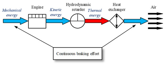 Figure 5. Energy flow of hydrodynamic retarder.The recommended standard operating fluid for hydrodynamic retarders in commercial vehicles is SJ 15W-40 gear oil, and its specification is as follows: the density is 860 kg/m3, the viscosity is 0.006 kg/m·s, the specific heat is 1884 J/(kg·k), and the thermal conductivity is 38 W/(m·k). When the temperature of the transmission fluid increases, the viscosity decreases and leads to the reduction of the pressure in the working chamber and that of the impact force on the blades, as well as an increase of the oil leaking and friction between components, which results in a decrease in the braking performance of the hydrodynamic retarder [30]. It is recommended to replace the heat exchange at a specified schedule and make sure that the viscosity and temperature are within a reasonable range (Figure 6) [31].
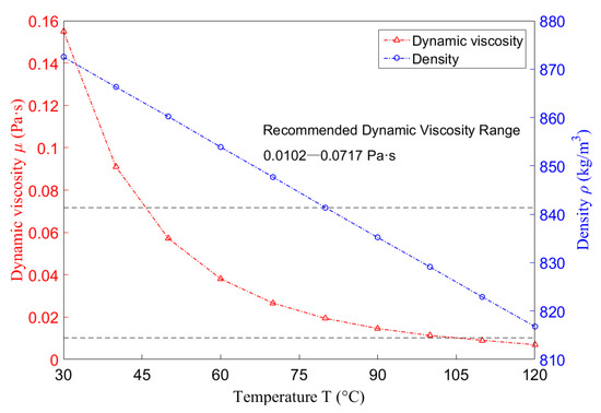 Figure 6. Density and viscosity of transmission fluid versus temperature.
- . Economy
- -
- . Weight G (kg):Weight reduction is identified as a way of improving product competitiveness and its ability to make profits. The reduction of the hydrodynamic retarder’s weight could decrease the vehicle’s mass, energy consumption, and duty levels on the brakes. The weight of the hydrodynamic retarder depends on its structure and material, which is mainly cast steel. For lightweight design, both the hydrodynamic retarder and its shell can be replaced with lighter materials such as polymers, cast aluminum, and cast steel, which will contribute to a more cost-effective system.
- -
- . Braking efficiency (%):The braking efficiency is the ratio of the input power to the actual output braking power, given by Equation (3).where is the input power that mainly comes from the oil supply system, and is the actual output braking power.The braking efficiency provides a measure of how efficiently the braking system utilizes energy to slow down or stop a vehicle. In addition to leakage of oil and mechanical wear on the transmission system, the primary dissipation of energy in the hydrodynamic retarder occurs within the internal flow field, including the friction and resistance between the oil impacting the blade and the viscous action of the oil’s physical properties [32]. The proper control mechanism can ensure that the retarder operates at its optimal efficiency, providing the necessary braking force while minimizing wear and tear. Moreover, higher fluid viscosity and lower temperature enhance the retarder’s effectiveness.
- -
- . Brake release time (s):The brake release time refers to the duration it takes to achieve the minimum braking torque once the brake pedal has been released, as shown in Figure 3. Generally, the brake release time of the hydrodynamic retarder should be less than 0.9 s. Prolonged brake release time can have negative effects on the subsequent acceleration process and result in increased fuel consumption. In activated and deactivated states of the hydrodynamic retarder, the effect factors would be the same in terms of the dynamic response of the entire system [33].
- -
- . Idling power loss (kW):In shut-off conditions, the control system discharges oil from the hydrodynamic retarder and fills the chamber with air, which could lead to a certain idling power loss, higher fuel consumption, and lower vehicle driving efficiency because of the undesirable air drag torque. The rotor of the hydrodynamic retarder is connected to the vehicle transmission, so the idling power loss increases with the rotational speed. The idling power loss is of the same principle as the generation of braking power [34]. Additional devices such as valve plates or spoilers are typically installed to minimize the idling power loss.
The criteria that will be used to evaluate hydrodynamic retarders are analyzed and quantified. The hierarchical structure is constructed correspondingly, as shown in Figure 7.
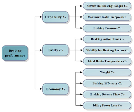
Figure 7.
Hierarchical structure of braking evaluation.
3. Performance Test
Multiple types of hydrodynamic retarders are available in the market today. To improve the representativeness of the sample to the population, the diversity of samples needs to be ensured. Therefore, sample A, sample B, and sample C selected as the hydrodynamic retarder alternatives in this paper are completely different in structure parameters. The schematic diagram of the three types of hydrodynamic retarders is shown in Figure 8. The structure parameters of the hydrodynamic retarder alternatives are listed in Table 1.
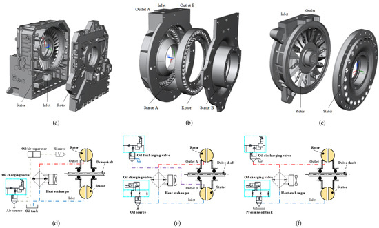
Figure 8.
Schematic diagram of three types of hydrodynamic retarders. (a) Sample A. (b) Sample B [35]. (c) Sample C [36]. (d) Schematic diagram of sample A. (e) Schematic diagram of sample B. (f) Schematic diagram of sample C.

Table 1.
Main parameters of three types of the hydrodynamic retarder systems.
Sample A is an in-line oil retarder with its own transmission-independent oil supply. Sample A holds an enormous advantage in that it is designed with a minimal impact on space claim and can be attached to any transmission [37]. When sample A is activated, the fluid in the oil tank is pressurized by the vehicle air system and is directed into the working chamber of the hydrodynamic retarder. The interaction of the fluid with the rotor and stator causes the rotor and output shaft to reduce speed on a downhill grade. When sample A is deactivated, the working chamber of the hydrodynamic retarder is evacuated, and the oil tank is recharged with fluid. Due to the fact that sample A is integrated into an independent cooling system, it will not impose additional requirements on the engine cooling system. The coolant flow coming from the outlet of the hydrodynamic retarder goes through the heat exchanger, and then back to the tank.
According to the number of torus, hydrodynamic retarders can be divided into single torus and dual torus types, also known as single chamber and dual chamber types. Sample B is a dual torus design, and the symmetrical double-sided impeller is rigidly connected to the output shaft of the gearbox. Two stators with blade sections are mounted on both sides of the rotor rigidly coupled with the gearbox housing. Compared with the single torus of sample A and sample C, sample B has the advantages of small radial size and great braking capacity and can also offset most axial force in the rotor, which improves the bearing force status. While straight blades are used in sample A and sample C, bowed blades are applied in the dual torus sample B. This design effectively reduces heat accumulation and blade stress, further decreasing maintenance time and cost and prolonging the service life to 4∼8 times [38]. The coolant flow is the result of the pressure differential that the transmission fluid creates between the inlet and outlet A, as shown in Figure 8b. The transmission fluid coming from outlet B of the hydrodynamic retarder goes through the oil discharging valve, and then back to the tank.
Sample C employs a pump/pressure tank in which the hydraulic fluid is under pressure at all times. Since this system can be brought into operation by opening a control valve, the hydraulic pressure does not have to build up from zero, and the time lag will be shorter compared to the pneumatic system of sample A. In addition, sample C has the maximum circulation heat dissipation and higher heat dissipation efficiency. The coolant flow coming from the outlet of the hydrodynamic retarder goes through the heat exchanger, and then back to the inlet of the hydrodynamic retarder.
The performance tests of the three types of hydrodynamic retarders are conducted to obtain evaluation values. In order to satisfy the requirements of any vehicles, the braking performance of hydrodynamic retarders shall be measured during tests conducted under the following conditions [39]:
- The tests shall be carried out at the rotational speeds, which shall not be less than 98% of the prescribed value. If the maximum design rotational speed of a hydrodynamic retarder is lower than the rotational speed prescribed for a test, the test shall be performed at the retarder’s maximum rotational speed.
- During the tests, the initial brake temperature of the hydrodynamic retarder shall be within 50 °C ± 1 °C, the average temperature of the hottest shell of the hydrodynamic retarder shall not exceed 120 °C and the instant temperature of the hottest shell of the hydrodynamic retarder shall not exceed 150 °C [40].
- The recording of all data shall be synchronized and be done after the hydrodynamic retarder runs fully and stably. Torque, rotational speed, pressure, flow, and temperature shall be recorded during the entire test using a data acquisition system at a sampling frequency of 50 Hz.
- The braking system control shall be designed such that its performance in use is not affected by the tester.
To ensure the rigor and accuracy of our testing procedure, we followed established standards throughout the idling power loss test and constant-torque braking test [41]. The above tests shall be repeated three times under the same conditions.
- Idling performance test:At the beginning of the test, ensure that the working chamber of the hydrodynamic retarder is idle and completely closed. Then gradually increase the rotational speed to 2500 rpm. The test parameter is idling power loss . The idling power losses of different retarder types in shut-off conditions are shown in Figure 9.
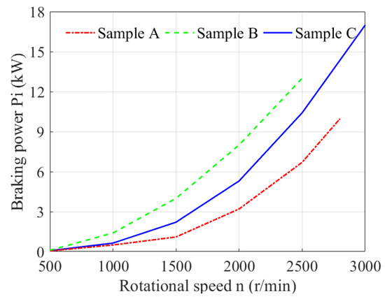 Figure 9. Idling power losses of different retarder types in shut-off conditions.
 - Constant-torque brake test:During the tests, the braking torque shall be maintained at a constant value of 1500 N·m, and the rotational speed is set to 1000 rpm due to the power limit of the motor. In addition, the braking time is set to 12 min according to ECE-R13 brake regulations [42]. Test parameters include: braking pressure , braking action time , stability for braking torque , final brake temperature , braking efficiency , and braking release time . The action time of the braking system shall be determined in a stationary state, the braking pressure is measured at the intake of sample A and the control oil circuit of the oil charging valve of sample B and sample C. The braking performance of different retarder types in constant-torque brake conditions is shown in Figure 10.
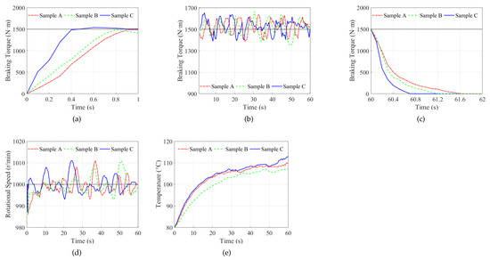 Figure 10. The braking performance of different retarder types in constant-torque brake conditions. (a) Constant-torque brake action stage. (b) Constant-torque brake stable stage. (c) Constant-torque brake release stage. (d) Rotational speed. (e) Temperature.
However, the rest parameters including weight , maximum braking torque and maximum input rotational speed were obtained from product manuals directly.
Each evaluation criterion has a performance rating for each attribute, which represents the characteristics of the criteria. It is common that performance ratings for different criteria are measured by different units, so it is necessary to quantify and standardize the criteria, and to make all the criteria comparable. The linear scale transformation method considers both the maximum and minimum performance ratings of the attributes during calculation. This method has the advantage that the scale measurement is precisely between 0 and 1 for each attribute [43]. Generally, evaluation criteria can be divided into benefit type and cost type. Benefit type refers to the criterion whose relative value is larger and better, and the cost type is the opposite. In this paper, , , , and are benefit type criteria; , , , , and are cost type criteria. For the convenience of plotting and subsequent data processing, the benefit type criteria are normalized using Equation (4), and the cost type criteria are normalized using Equation (5).
where is the maximum performance rating among the alternatives for attribute and is the minimum performance rating among the alternatives for attribute .
The test results and normalization results of evaluation criteria are shown in Table 2.
Table 2.
Test results and normalization results for each criterion.
4. Fuzzy Analytic Hierarchy Process (FAHP)
This paper utilizes the four-step FAHP method to determine the weights of the criteria. Experts are required to provide their judgments on the basis of their expertise and to compare every factor pairwise in their corresponding section structured in the hierarchy. Then these experts’ preferences are converted into a fuzzy number evaluation matrix. The defuzzication is employed to transform the fuzzy scales into crisp scales for the computation of priority weights.
Let be an object set and be a goal set. According to the method of Chang’s extent analysis [44], each object is taken, and extent analysis for each goal is performed, respectively. Therefore, m extent analysis values for each object can be obtained with the following signs:
where all the are triangular fuzzy numbers expressed as a triple . Here m, u, and l are the mean, the lower, and the upper bounds, respectively. A fuzzy set is defined by its membership function as the following [45,46]
The procedure of FAHP are described as follows [47]:
- Perform extent analysis for each goal, respectively. The fuzzy synthetic extent with respect to ith object is defined as
- Evaluate the degree of possibility for fuzzily restricted to belong to M to be greater than fuzzily restricted to belong to M. The degree of possibility of is defined asIn addition, it can be equivalently expressed as follows:where d is the ordinate of highest intersection point D between and , as shown in Figure 11. To compare and , we need both the values of and .
 Figure 11. The intersection between and [48].
 - Calculate the priority weights of criteria. The degree of possibility for a convex fuzzy number to be greater than k convex fuzzy number can be defined byAssume thatfor . Then the weight vector is given bywhere are n elements.
- The normalized weight vector is calculated aswhere W is a non-fuzzy vector.
5. Improved Radar Chart
The principle of the traditional radar chart method is to take the sector radius as the axis and calibrate the quantitative value of each criterion on its corresponding criterion axis. Subsequently, these points are interconnected to create a closed polygon, resulting in the generation of the evaluation object’s radar chart, as shown in Figure 12. This paper advances the conventional radar chart method even further. The analysis process of the IRC comprises the following steps:
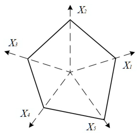
Figure 12.
Traditional radar chart.
- The unit circle is divided into n sectors based on the selected n criteria, with each sector region as the criterion’s corresponding domain. The weights () of the evaluation criteria are then converted into central angles () using the formula .
- The sector radius is used as the axis, and the standardized quantitative value of each criterion is calibrated on the corresponding criterion axis.
- The calibration value is taken as the radius (), and the central angle () is determined according to the weight, which is used to draw the circular arc, as shown in Figure 13.
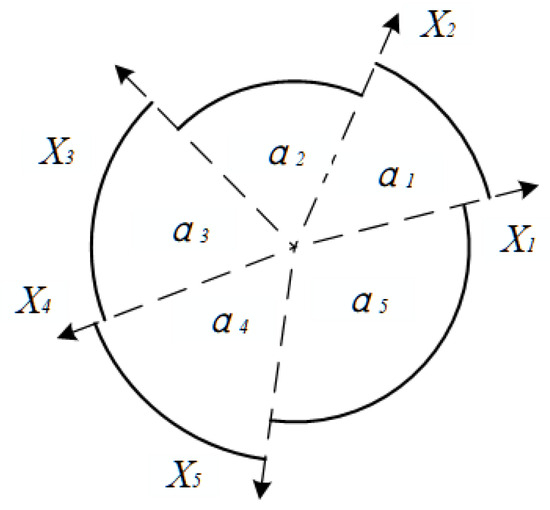 Figure 13. Improved radar chart.
 - The evaluation result is obtained by constructing eigenvectors using the area and perimeter of the IRC [49].From an improved radar chart, we can extract the area and the perimeter , which respectively symbolize the comprehensive advantages of the evaluation object and the equilibrium among the variations in each evaluation criterion. The constructed eigenvector is given byAccording to the constructed eigenvector, the evaluation vector is defined aswhere is the area evaluation value. A greater value corresponds to an elevated level of comprehensiveness in the evaluation object. Similarly, is the perimeter evaluation value. A larger value indicates a greater balance in the variations of the evaluation object’s criteria. Consequently, the evaluation vector integrates both the overall change degree of the evaluation object and the equilibrium degree of each criterion.The evaluation function is formulated using the geometric mean method, and its definition is presented as follows:
6. Application
Three decision-makers with diverse backgrounds and extensive experience in the field of hydrodynamic retarders are carefully selected to participate in the evaluation process. Decision-maker 1 holds a Ph.D. and has over thirty years of research experience in fluid power transmission. Decision-maker 2 is an engineer with a background in product production, contributing to the development of tests and evaluations. Decision-maker 3 is a product salesperson who understands the market trends and the consumers’ needs. Each decision-maker () individually carry out pairwise comparisons using Saaty’s 1∼9 scale. The meaning of 1∼9 scales are illustrated in Table 3.
Table 3.
Saaty’s scale for pairwise comparison [50].
The pairwise comparisons of the main criteria are shown as follows:
The consistency ratio (CR) is employed to verify the consistency of the pairwise comparisons made by the experts’ judgments. The comparison of the consistency index with a random generator (RI) value, as established by Saaty, is listed in Table 4.
where is the consistency index, is the maximum eigenvalue, n is the size of matrix. If the is less than 10%, this means that the inconsistency in comparisons in the decision-making matrix is considered acceptable. Otherwise, the experts are contacted again to review their comparisons. The values of the pairwise comparisons demonstrates the suitability of the proposed consistency index.
Table 4.
Random index for different matrix sizes [51].
Then, a comprehensive pairwise comparison matrix is constructed, as illustrated in Table 5, by integrating three decision-makers’ grades through Equation (21). In this way, the decision-makers’ pairwise comparison values are transformed into triangular fuzzy numbers.
where is the evaluation of objectives , by the decision-maker.
Table 5.
Fuzzy pairwise comparison matrix criteria for all decision-makers.
Following the creation of the fuzzy pairwise comparison matrix, weights of all criteria and sub-criteria are determined by the FAHP methodology. Utilizing the data in Table 5, synthesis values corresponding to the main goal are computed through Equation (8):
These fuzzy values are compared using Equation (10):
Then, priority weights are calculated by using Equation (12):
The weights of the main criteria . Upon normalizing these values, the weights corresponding to the main goal are derived as . It is found from the study that safety proved to be the most crucial factor for the selection of brake performance. Finally, summing the weights of each main criterion multiplied by the weights of their corresponding sub-criteria results in the overall weight. The aggregated weights and consistency ratios for each criterion are shown in Table 6. The results indicate that braking action time has the most remarkable impact on braking performance, followed by the maximum braking torque and braking efficiency . This is because the primary function of a hydrodynamic retarder is to slow or stop the vehicle as soon as possible, and the braking action time is strongly connected to the stop distance. Long stop distances may result in traffic accidents. However, braking pressure , final brake temperature , braking release time , and idling power loss are of equal importance for sustaining high braking performance. Therefore, the whole vehicle’s design also must ensure that the cooling system of the hydrodynamic retarder meets braking power requirements and less energy consumption of hydrodynamic retarder in the deactivated state. Stability for braking torque and weight are of less importance while improving braking performance.
Table 6.
Aggregated weights and consistency ratios.
The data in Table 2 and Table 6 are mapped onto the IRC, as shown in Figure 14a. The results show that sample C can offer an option to heavy-duty vehicles that will reduce overall operating costs, improve driveability and enhance the safety of the entire vehicle. The comprehensive assessment outcome for both sample A and sample B is remarkably similar, but sample B exhibits superiority over sample A in terms of the proportionality of all indices. Utilizing Equation (17), calculations for the area and perimeter of the colored parts within the IRC are performed, thereby extracting the evaluation results () for each IRC. The performance ranking order of the three hydrodynamic retarders is sample C (ER = 0.675) ≻ sample A (ER = 0.564) ≻ sample B (ER = 0.561), as shown in Figure 14b. The height of a rectangle signifies the weight of the corresponding criterion. The weights of the criteria are 0.334 for Capability, 0.345 for Safety, and 0.321 for Economy. It is evident that sample B excels in safety, but lags in capability and economy. Sample B exhibits lower performance values in terms of maximum braking torque and maximum input rotational speed , while these are important factors, according to the experts. This leads to the comparatively inferior braking performance of sample B among the three hydrodynamic retarders.
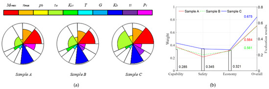
Figure 14.
Performance graphic of three types of hydrodynamic retarders. (a) Improved radar chart. (b) Evaluation results.
Sensitivity Analysis
Due to the weights of the criteria changing continuously throughout the project ranking process, the ranking results may also adapt accordingly. Following the acquisition of the initial solution with the established criterion weights, sensitivity analyses are executed to investigate how the overall prioritization of alternatives responds to variations in the relative synthesis value of each criterion. In the following, a sensitivity analysis is carried out to examine the robustness and reliability of the braking performance selection process for hydrodynamic retarders.
Using the perturbation method, the reasonable range of weights for each criterion is obtained, and the associated data are shown in Table 7. The weight perturbation momentum is set to 0.01 as the basic unit, while the minimum weight of each criterion is set to 0.025. It is important to note that when adjusting the weight of a single criterion, the weights of all criteria should be normalized to ensure the consistency of the weighting scheme.
Table 7.
Weight range for each criterion.
When the weight of the Capability criterion is decreased from 0.334 to 0.285 or less (Figure 15a), or the weight of the Safety criterion is increased from 0.345 to 0.373 or more (Figure 15b), or the weight of the Economy criterion is decreased from 0.321 to 0.242 or less (Figure 15c), sample A takes the third rank. On the other hand, Sample C consistently maintains its leading position regardless of fluctuations in the weights of other criteria. The results of the sensitivity analysis reveal that the braking performance evaluation system of hydrodynamic retarders displays a relatively low sensitivity to alterations in criteria weights. Furthermore, the ranking result proves most responsive to variations in the weight of the Safety criterion, while it is the least sensitive to changes in the weight of the Economy criterion. This highlights the critical importance of the Safety criterion in determining the ranking of braking performance for hydrodynamic retarders.
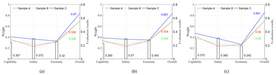
Figure 15.
Results of weight sensitivity analysis. (a) Sensitivity results for the criterion “Capability”. (b) Sensitivity results for the criterion “Safety”. (c) Sensitivity results for the criterion “Economy”.
7. Discussion and Conclusions
A novel braking performance evaluation method is developed to conduct a more comprehensive analysis of hydrodynamic retarder. This paper identifies evaluation criteria and establishes the evaluation criteria hierarchy of braking performance of hydrodynamic retarders. The fuzzy analytic hierarchy process is used to determine the weights of evaluation criteria, and the results highlighted the most influential criteria and sub-criteria, namely safety and braking action time. The improved radar chart method is employed to comprehensively evaluate and rank the performance. Sensitivity analysis is also performed to investigate the sensitivity of the ranking results to changes in the weights of main criteria. An actual case example of three types of hydrodynamic retarders is presented. The result shows the practicality of the established evaluation criteria hierarchy and validates the effectiveness and feasibility of the proposed method. The evaluation criteria and the determination weights provide a valuable reference for multi-objective optimization control strategies and structural optimal design of hydrodynamic retarders. The ranking result of different hydrodynamic retarders offers practical guidance for managers.
However, some limitations can be expected. The evaluation of the braking performance of hydrodynamic retarders is an extremely time-consuming and complex task that involves a wide range of knowledge. The proposed method did not consider all possible criteria that could be added to the model. The criteria may include human factors such as driver behavior reaction times, and the influence of various factors such as distraction or fatigue on braking performance. In addition, the ranking of the alternatives may change if a new criterion is added.
For future work, we intend to explore more cases and conduct more empirical studies to further validate the usefulness of the research. In addition, the problem could be extended with the other outranking MCDM methods.
Author Contributions
Conceptualization, Z.W. and W.W.; methodology, Z.W. and R.L.; software, Z.W. and R.L.; validation, W.W. and X.C.; formal analysis, Z.W.; investigation, X.C.; resources, W.W. and Q.Y.; data curation, W.W. and X.C.; writing—original draft preparation, Z.W.; writing—review and editing, Q.Y. and R.L.; visualization, Z.W.; supervision, Q.Y.; project administration, W.W.; funding acquisition, W.W. and Q.Y. All authors have read and agreed to the published version of the manuscript.
Funding
This research was funded by the National Natural Science Foundation of China, grant numbers 51475041 and 51805027.
Institutional Review Board Statement
Not applicable.
Informed Consent Statement
Not applicable.
Data Availability Statement
Not applicable.
Acknowledgments
This research was supported by the Beijing Institute of Technology Joint Ph.D Student Training Scholarship.
Conflicts of Interest
The authors declare no conflict of interest.
References
- Lechner, G.; Naunheimer, H. Automotive Transmissions: Fundamentals, Selection, Design and Application; Springer Science & Business Media: Berlin, Germany, 1999; pp. 309–312. [Google Scholar]
- Wang, Y.; Lin, L. The evaluation of braking performances of mechanical brake system on oil rig. J. Adv. Mech. Des. Syst. Manuf. 2013, 7, 195–204. [Google Scholar] [CrossRef][Green Version]
- Jeon, K.; Park, J.I.; Choi, S.; Yi, K. Electronic brake safety index for evaluating fail-safe control of brake-by-wire systems for improvement in the straight braking stability. Proc. Inst. Mech. Eng. Part D J. Automob. Eng. 2014, 228, 873–893. [Google Scholar] [CrossRef]
- Jia, P. An Approach for Heavy-Duty Vehicle-Level Engine Brake Performance Evaluation. SAE Int. J. Commer. Veh. 2019, 12, 57–67. [Google Scholar] [CrossRef]
- Kahraman, C.; Kaya, İ.; Cebi, S. A comparative analysis for multiattribute selection among renewable energy alternatives using fuzzy axiomatic design and fuzzy analytic hierarchy process. Energy 2009, 34, 1603–1616. [Google Scholar] [CrossRef]
- Watróbski, J.; Jankowski, J.; Ziemba, P.; Karczmarczyk, A.; Ziolo, M. Generalised framework for multi-criteria method selection. Omega 2019, 86, 107–124. [Google Scholar] [CrossRef]
- Mosadeghi, R.; Warnken, J.; Tomlinson, R.; Mirfenderesk, H. Comparison of Fuzzy-AHP and AHP in a spatial multi-criteria decision making model for urban land-use planning. Comput. Environ. Urban Syst. 2015, 49, 54–65. [Google Scholar] [CrossRef]
- Ayan, B.; Abacıoğlu, S.; Basilio, M.P. A Comprehensive Review of the Novel Weighting Methods for Multi-Criteria Decision-Making. Information 2023, 14, 285. [Google Scholar] [CrossRef]
- Lai, Y.J.; Liu, T.Y.; Hwang, C.L. Topsis for MODM. Eur. J. Oper. Res. 1994, 76, 486–500. [Google Scholar] [CrossRef]
- Saaty, T.L. What is the analytic hierarchy process? In Mathematical Models for Decision Support; Springer: Berlin/Heidelberg, Germany, 1988; pp. 109–121. [Google Scholar]
- Hendre, K.; Bachchhav, B. Critical property assessment of novel brake pad materials by AHP. J. Manuf. Eng. 2018, 13, 148–151. [Google Scholar]
- Ooi, J.; Promentilla, M.A.B.; Tan, R.R.; Ng, D.K.; Chemmangattuvalappil, N.G. Integration of fuzzy analytic hierarchy process into multi-objective computer aided molecular design. Comput. Chem. Eng. 2018, 109, 191–202. [Google Scholar] [CrossRef]
- Wu, H.Y.; Tzeng, G.H.; Chen, Y.H. A fuzzy MCDM approach for evaluating banking performance based on Balanced Scorecard. Expert Syst. Appl. 2009, 36, 10135–10147. [Google Scholar] [CrossRef]
- Shaojie, W.; Liang, H.; Lee, J.; Xiangjian, B. Evaluating wheel loader operating conditions based on radar chart. Autom. Constr. 2017, 84, 42–49. [Google Scholar]
- Chaumillon, R.; Romeas, T.; Paillard, C.; Bernardin, D.; Giraudet, G.; Bouchard, J.F.; Faubert, J. Enhancing data visualisation to capture the simulator sickness phenomenon: On the usefulness of radar charts. Data Brief 2017, 13, 301–305. [Google Scholar] [CrossRef]
- Wang, Y.L.; Li, Y.J. Comprehensive Evaluation of Power Transmission and Transformation Project Based on Improved Radar Chart. Adv. Mater. Res. 2011, 354–355, 1068–1072. [Google Scholar] [CrossRef]
- Zhang, X.; Jiang, Y.; Wang, X.B.; Li, C.; Zhang, J. Health Condition Assessment for Pumped Storage Units Using Multihead Self-Attentive Mechanism and Improved Radar Chart. IEEE Trans. Ind. Inform. 2022, 18, 8087–8097. [Google Scholar] [CrossRef]
- Chunbao, L.; Linshan, G.; Wenxing, M.; Xuesong, L. Multiobjective optimization design of double-row blades hydraulic retarder with surrogate model. Adv. Mech. Eng. 2015, 7, 1. [Google Scholar] [CrossRef]
- Gao, Z.; Li, D.; Liu, Z.; Ye, L. Design and Braking Stability Analysis of a Novel Internal Pump-Hydraulic Retarder Axle for Heavy Articulated Vehicle. Int. J. Automot. Technol. 2022, 23, 1285–1294. [Google Scholar] [CrossRef]
- Fancher, P.; O’Day, J.; Bunch, H.; Sayers, M.; Winkler, C. Retarders for Heavy Vehicles: Evaluation of Performance Characteristics and In-Service Costs; Volume I: Technical Report; SAE Technical Report; The University of Michigan: Ann Arbor, MI, USA, 1981. [Google Scholar]
- Liu, C.; Bu, W.; Wang, T. Numerical investigation on effects of thermophysical properties on fluid flow in hydraulic retarder. Int. J. Heat Mass Transf. 2017, 114, 1146–1158. [Google Scholar] [CrossRef]
- Chen, M.; Guo, X.; Tan, G.; Pei, X.; Zhang, W. Effects of blade lean angle on a hydraulic retarder. Adv. Mech. Eng. 2016, 8, 2–3. [Google Scholar] [CrossRef]
- ISO 611; Road Vehicles-Braking of Automotive Vehicles and Their Trailers—Vocabulary. ISO/TC 22/SC 33 Vehicle Dynamics and Chassis Components; ISO: Geneva, Switzerland, 2003.
- GB 7258-2017; Safety Specifications for Safety of Power-Driven Vehicles Operating on Roads. National Standard of the People’s Republic of China: Beijing, China, 2012.
- Limpert, R. Analysis and Design of Automotive Brake Systems; The US Army Materiel Development and Readiness Command: Alexandria, Virginia, 1985.
- Haiss, J. Demand Criteria on Retarders; Technical Report, SAE Technical Paper; SAE International: Warrendale, PA, USA, 1992. [Google Scholar]
- Akers, A.; Gassman, M.; Smith, R. Hydraulic Power System Analysis; CRC Press: Boca Raton, FL, USA, 2006; pp. 82–89. [Google Scholar]
- Kong, L.; Wei, W.; Yan, Q. Application of flow field decomposition and reconstruction in studying and modeling the characteristics of a cartridge valve. Eng. Appl. Comput. Fluid Mech. 2018, 12, 385–396. [Google Scholar] [CrossRef]
- Mu, H.; Wei, W.; Kong, L.; Zhao, Y.; Yan, Q. Braking characteristics integrating open working chamber model and hydraulic control system model in a hydrodynamic retarder. Proc. Inst. Mech. Eng. Part C J. Mech. Eng. Sci. 2019, 233, 1952–1971. [Google Scholar] [CrossRef]
- Bu, W.; Shen, G.; Qiu, H.; Liu, C. Investigation on the dynamic influence of thermophysical properties of transmission medium on the internal flow field for hydraulic retarder. Int. J. Heat Mass Transf. 2018, 126, 1367–1376. [Google Scholar] [CrossRef]
- Danfoss. Hydraulic Fluids and Lubricants-Oils, Lubricants, Grease, Jelly; Engineering Tomorrow: Fairfax Station, VA, USA, 2016. [Google Scholar]
- Liu, Z.; Zheng, H.; Xu, W.; Yu, Z. A Downhill Brake Strategy Focusing on Temperature and Wear Loss Control of Brake Systems; Technical Report, SAE Technical Paper; SAE International: Warrendale, PA, USA, 2013. [Google Scholar]
- Clarke, R.; Radlinski, R.W.; Knipling, R. Improved Brake Systems for Commercial Motor Vehicles; Technical Report; National Highway Traffic Safety Administration: Washington, DC, USA, 1991.
- An, Y.; Wei, W.; Li, S.; Liu, C.; Meng, X.; Yan, Q. Research on the mechanism of drag reduction and efficiency improvement of hydraulic retarders with bionic non-smooth surface spoilers. Eng. Appl. Comput. Fluid Mech. 2020, 14, 447–461. [Google Scholar] [CrossRef]
- Yan, Q.; Mu, H.; Wei, W. Comparative analysis of braking performance for dual torus hydrodynamic retarder with bowed blade and straight blade. In Proceedings of the 2015 International Conference on Fluid Power and Mechatronics (FPM), Harbin, China, 5–7 August 2015; IEEE: Piscataway, NJ, USA, 2015; pp. 123–127. [Google Scholar]
- Wei, W.; Li, Y.; An, Y.; Guo, D.; Yan, Q. Research on the Influence Law of Cascade Parameters on the Onset Characteristics of Hydrodynamic Retarder. J. Mech. Eng. 2023, 59, 265–266. [Google Scholar]
- Turbo, V. Voith Retarder R 133-2 Service Manual; Voith Turbo GmbH & Co. KG: Heidenheim an der Brenz, Germany, 2010. [Google Scholar]
- Cooney, T.J.; Mazzali, P. The MT643R-An Automatic Transmission with Retarder for the Latin American Market; Technical Report, SAE Technical Paper; SAE International: Warrendale, PA, USA, 1997. [Google Scholar]
- GB/T 32692-2016; Performance Test Methods for Endurance Braking Systems of Commercial Vehicles. National Standard of the People’s Republic of China: Beijing, China, 2016.
- National Highway Traffic Safety Administration. Federal Motor Vehicle Safety Standards 105; National Highway Traffic Safety Administration: Washington, DC, USA, 2006.
- QC/T 1046-2016; Performance Requirements and Bench Test Methods for Commercial Vehicle Secondary Hydraulic Retarder. National Standard of the People’s Republic of China: Beijing, China, 2016.
- GB/T 25627-2010; Construction Machinery-Power-Shift Transmissions. National Standard of the People’s Republic of China: Beijing, China, 2010.
- Tzeng, G.H.; Huang, J.J. Multiple Attribute Decision Making: Methods and Applications; CRC Press: Boca Raton, FL, USA, 2011; p. 69. [Google Scholar]
- Chang, D.Y. Extent analysis and synthetic decision. Optim. Tech. Appl. 1992, 1, 352–355. [Google Scholar]
- Chen, G.; Pham, T.T.; Boustany, N. Introduction to fuzzy sets, fuzzy logic, and fuzzy control systems. Appl. Mech. Rev. 2001, 54, B102–B103. [Google Scholar] [CrossRef]
- Zadeh, L.A. Information and control. Fuzzy Sets 1965, 8, 338–353. [Google Scholar]
- Leśniak, A.; Kubek, D.; Plebankiewicz, E.; Zima, K.; Belniak, S. Fuzzy AHP application for supporting contractors’ bidding decision. Symmetry 2018, 10, 642. [Google Scholar] [CrossRef]
- Saaty, T.L. Decision making with the analytic hierarchy process. Int. J. Serv. Sci. 2008, 1, 83–98. [Google Scholar] [CrossRef]
- Wang, Q.; Guan, Z.; Zhang, B.; Liu, Y.; Li, C. Multilevel method based on improved radar chart to evaluate acoustic frequency spectrum in periodic pipe structure. J. Pet. Sci. Eng. 2020, 189, 7–9. [Google Scholar] [CrossRef]
- Saaty, T.L.; Vargas, L.G. Models, Methods, Concepts & Applications of the Analytic Hierarchy Process; Springer Science & Business Media: New York, NY, USA, 2012; Volume 175, p. 6. [Google Scholar]
- Saaty, T.L.; Kearns, K.P. Analytical Planning: The Organization of System; Elsevier: New York, NY, USA, 2014; Volume 7, p. 34. [Google Scholar]
Disclaimer/Publisher’s Note: The statements, opinions and data contained in all publications are solely those of the individual author(s) and contributor(s) and not of MDPI and/or the editor(s). MDPI and/or the editor(s) disclaim responsibility for any injury to people or property resulting from any ideas, methods, instructions or products referred to in the content. |
© 2023 by the authors. Licensee MDPI, Basel, Switzerland. This article is an open access article distributed under the terms and conditions of the Creative Commons Attribution (CC BY) license (https://creativecommons.org/licenses/by/4.0/).