LSTM-Based Condition Monitoring and Fault Prognostics of Rolling Element Bearings Using Raw Vibrational Data

Abstract

The 4.0 industry revolution and the prevailing technological advancements have made industrial units more intricate. These complex electro-mechanical units now aim to improve efficiency and increase reliability. Downtime of such essential units in the current competitive age is unaffordable. The paradigm of fault diagnostics is being shifted from conventional to proactive predictive approaches. As a result, Condition-based Monitoring and prognostics are now essential components of complex industrial systems. This research is focused on developing a fault prognostic system using Long Short-Term Memory for rolling element bearings because they are a critical component of industrial systems and have one of the highest fault frequencies. Compared to other research, feature engineering is minimized by using raw time series sensor data as an input to the model. Our model achieved the lowest root mean square error and outperformed similar research models where time domain, frequency domain, or time-frequency domain features were used as input to the model. Furthermore, using raw vibration data also enabled better generalization of the model. This has been confirmed by evaluating the performance of the developed model against vibration data generated by distinct sources, including hydro and wind power turbines.

1. Introduction

One of the most important components in industrial machines are bearings, which normally operate under a very stressful environment and, hence, are continuously prone to degradation [1]. Thus, bearings are among the few critical and foremost fault-causing components in electro-mechanical systems [2]. When aged, faults like bearing wear and tear and symptoms, such as abnormal vibrations, high temperatures, and misalignments, are introduced into the system. Therefore, a predictive approach toward fault identification is necessary in modern, industrially-revolutionized times to avoid forced downtime.

The existing Condition-based Monitoring (CBM) and system health monitoring approaches are generically classified into (1) physics-based models that require extensive domain knowledge where the models are constructed using mathematical equations, and (2) data-driven models where the training of the model is conducted using historic data generated by the sensors [3,4] because the data-driven models work with historic sensory data collected from the machines. Such data can be recorded online, where the model’s parameters can be updated in real-time. Therefore, this approach makes the data-driven models more attractive for the predictive maintenance of electro-mechanical machines.

Various models have been developed for the effective condition monitoring of bearings, including acoustic emission-based models [5,6]. However, vibration signal analysis [7,8] is one of the most widely used and most effective methods to conduct the prognosis of rotating machines. The occurrence of faults in the rotating machines can result in machine downtime and is directly related to higher operation and maintenance (O&M) costs, serious accidents, and economic losses [9,10]. The fault diagnosis in rotating machines can therefore be conducted by measuring the speed variations using speed sensors [11,12] or by quantifying the vibration signals using accelerometers [13]. However, fault detection and prognostics using vibration signals are the most widely used approaches. A detailed review of the feature extraction and selection techniques, different classifiers, and deep learning models using the Case Western Reserve University bearing center (CWRU) dataset was conducted [14]. Similarly, a future roadmap for intelligent fault diagnostics has been provided [15], and a systematic review of the recent advancements in mechanical fault diagnostics and prognostics was carried out [16].

Several techniques have been adopted to identify faults in the vibration data, including short-time Fourier transform (STFT) and wavelet transform [17,18,19,20]. Among the other adapted approaches are band-pass filtering, phase demodulation, Kalman filters, and deep learning techniques based on deep neural networks [21,22,23,24,25]. A total of 17 different classifiers using the MATLAB Classification Learner toolbox along with support vector machine (SVM), K-nearest neighbors (KNN), and ensemble have been used to evaluate the performance of classifiers for diagnosing the faults in induction motors [26]. Likewise, classical machine learning algorithms have also been used to detect leakages in the waterwall tube of a steam power plant [27].

As computational resources advance, deep learning has been in the spotlight, especially in the area of prognostics, because of its effectiveness in modeling complex systems [28]. Artificial neural networks (ANNs) are the most common deep learning methods used for prognostics because of their outstanding performance against complex non-linear multi-dimensional systems. Their ability to effectively process non-linear information makes them more robust concerning noise. Many ANN architectures, such as Feed-forward, Single and Multilayer Perceptron, Recurrent Neural Networks (RNNs), Long Short-Term Memory (LSTM), Modular Neural Networks (MNNs), and Convolutional Neural Networks (CNNs), are being used to conduct the CBM and prognostics of industrial and renewable energy systems [29]. To diagnose the bearing faults, a large memory storage retrieval (LAMSTAR) neural network based on an optimized deep learning structure is proposed [30]. A Bayesian deep learning model to characterize the latent structure between RULs and degradation features is used to describe prognostic uncertainties [31]. Based thereon, dynamic decisions pertinent to maintenance and spare-part ordering are taken. The performance of the proposed framework has been validated through comparison with various benchmarking policies based on a C-MAPSS turbofan engine data set. Extensive research on integrating Artificial Intelligence, Big Data, and the Industrial Internet of Things in smart manufacturing and modern dynamic industrial processes and energy generation units under the umbrella of Industry 4.0 is conducted [32]. The issue of data imbalances is solved using virtual sensors to artificially induce different health states in the vibration data [33].

This research, therefore, focused on developing a dynamic and robust prognostic model that can efficiently predict the degradation and faults of the bearings based on the raw vibration data recorded from the sensors. All analyses in this research were conducted in the time domain, and the need for feature engineering was minimized by taking actual sensor data as input. The proposed model was developed to predict the bearing degradation and faults ahead of time. Because the raw vibration data generated by the sensors were used for model training and testing, the model could be effectively generalized. To evaluate the generalization capabilities of the developed model, the model was tested for analyzing the faults in the bearings of both hydro and wind power turbines. It was observed that the model effectively predicted the bearing vibration values irrespective of the data source. Using raw vibration values instead of time-domain features also has an advantage in cases where condition monitoring is carried out online in real-time. Since, at any instant in time, only partial data is available, effectively acquiring time-domain features becomes a difficult ask.

The remaining part of the paper is organized as follows. Section 1.1 discusses the novelty of the research. Section 2 explains the overall methodology, including the justification and architecture of the proposed model. Section 3 explains the process of data acquisition, details about the dataset, and elaborates the experimental setup. Section 3 explains the evaluation metrics and results and also compares the results with those achieved by similar research. The generalization ability of the model is also discussed in Section 3. Finally, the paper is concluded in Section 4.

1.1. Related Research and Novelty

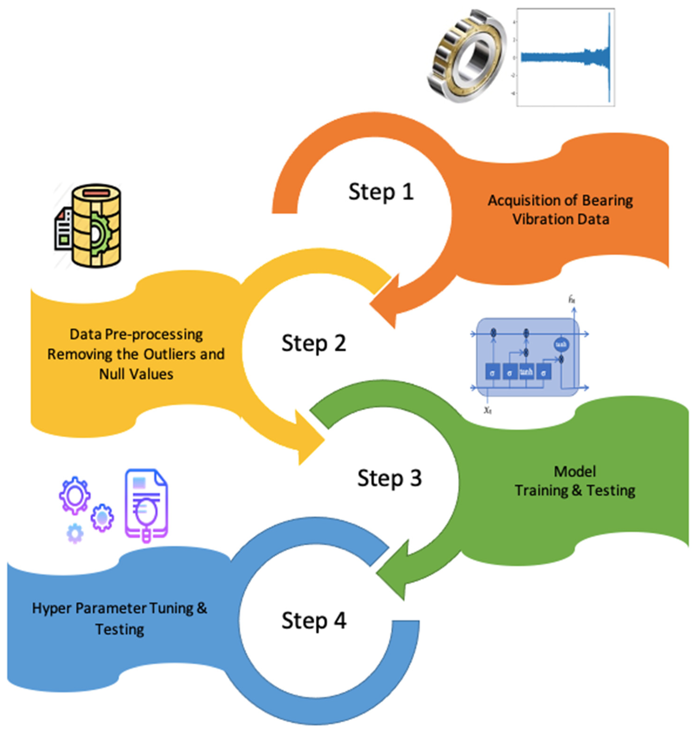
Previous research conducted on bearing vibration datasets mostly focused on the frequency domain [34,35]. At first, the time-series data were converted into the frequency domain, followed by data pre-processing and feature extraction [34]. Such analysis is based on the pretext that the data components with higher frequency are actually the added system noise. Subsequently, low-pass filters were used to remove these higher-frequency components, segregating the system and bearing vibrations. However, in a realistic environment, the vibration signals generated by the machinery (other than the bearings) are an integral part of the data. Segregation of these system vibration signals from the bearing vibration signals requires an extensive domain knowledge and, hence, is highly prone to errors.

Furthermore, in similar research, either time domain features, frequency domain features, or time–frequency domain features, such as mean, standard deviation, kurtosis, and skewness, were considered input(s) to the model [36,37,38,39,40,41]. However, in cases where prognostics are conducted in real-time, where only partial data generated by the Supervisory Control and Data Acquisition (SCADA) system are available at any time, such statistical feature extraction cannot be carried out effectively.

Therefore, this research concentrated on conducting the model training and testing using the actual raw sensor data as an input to the model. This approach helped reduce the need for extensive feature engineering and domain knowledge and also improved the performance of the model in terms of root mean square error (RMSE). Furthermore, because the model is trained using raw sensor data, it can be effectively generalized. An in-depth analysis of the results and generalization capabilities, along with comparing the results with other similar models, are given in later sections.

2. Methodology

The model was developed and tested using Python programming language. The prediction of the vibration values was carried out by first acquiring the sensory data containing raw vibration values recorded by a test rig. Subsequently, this raw data was pre-processed for the removal of any outliers. The pre-processed data were normalized and then used to train and test a prognostic model based on a machine-learning algorithm. Finally, hyper-parameter testing and fine-tuning of the model were conducted. In the end, the generalization capability of the model was verified by testing it against real vibration data generated by different sources.

Figure 1 shows the flow chart of the methodology, comprising the experimental steps.

Figure 1. Steps of the methodology.

2.1. Model Selection

The vibration signals generated by the installed sensors represent the time-series data expressed sequentially. One of the limitations of conventional models based on multi-domain feature extraction, including kurtosis, spectral skewness, and wavelet coefficients, is their ineffectiveness to model the inherent sequential characteristics of the sensory data. Moreover, selecting features for these models requires extensive domain knowledge and feature engineering skills.

Furthermore, the sequential models, including the traditional ANNs, hidden Markov models (HMMs), Kalman filters, and conditional random fields, despite having their ability to handle the sequential data, are incapable of addressing the long-term dependencies. As in machine condition monitoring based on sensory data, many noisy or non-discriminative signals may exist between two consecutive informative or discriminative signals. Hence, a long delay on a time scale is induced between important data points. This leads to reduced efficiency and performance of the aforementioned models when working with the time series data.

To address the issues of long-term data dependency, the use of RNNs for handling sequential data has increased substantially [42]. However, one of the shortcomings of RNNs is the problem of gradient exploding and vanishing. Although RNNs can store the previous inputs in the network and can be trained using backpropagation, their ability to cater to long-term dependencies in sequential data is reduced because of the gradient vanishing problem.

Consequently, the LSTM algorithm was introduced [43]. This algorithm prevented the gradient from vanishing or exploding; however, it also addressed the long-term data dependencies by introducing forget gates in the architecture. LSTMs can simultaneously carry out representative learning and model training without additional domain knowledge. Regarding the unprecedented performance against time-series data, the LSTM algorithm was used to develop the prognostic model.

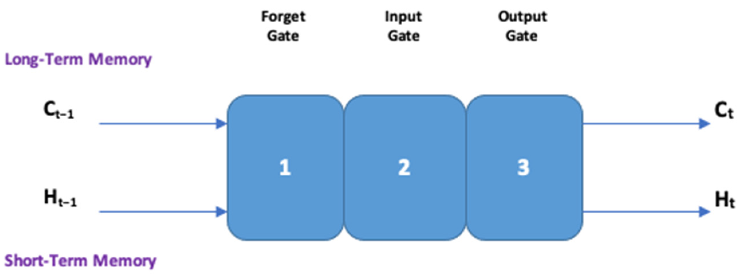
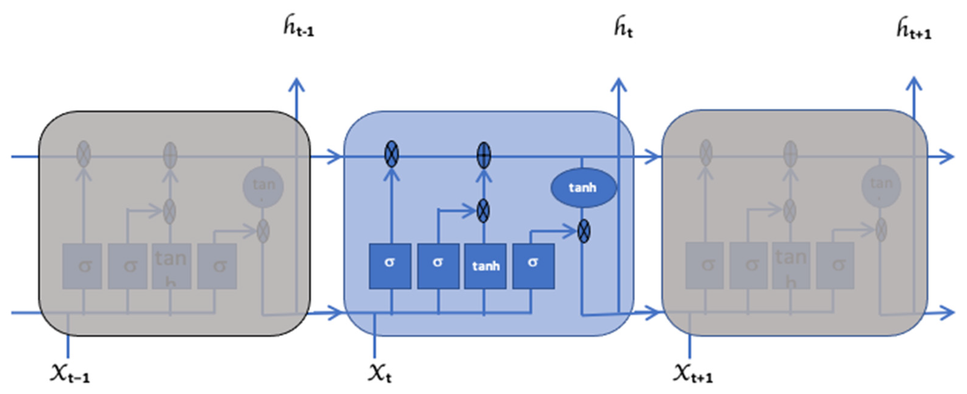
2.2. Long Short-Term Memory (LSTM)

LSTM was first presented in 1997 by Hochreiter and Schmidhuber [43]. It is a type of RNN that can effectively establish a correlation between a priori information and the current state based on a time series. The proposed LSTM network comprises three basic components, the Forget gate, Input gate, and Output gate, as shown in Figure 2. These components are used to (1) Forget irrelevant information, (2) Add/Update new information, and (3) Pass on the updated information.

Figure 2. Basic layout of the proposed LSTM network.

• where:
• C_t−1 represents the cell state of the previous timestamp;
• H_t−1 represents the hidden state of the previous timestamp;
• C_t represents the current cell state;
• H_t represents the current hidden state.

The cell state carries the information, in our case the vibration data points along with all timestamps, and is known as long-term memory. The hidden state is known as short-term memory, hence the name Long Short-Term Memory.

Along with some minor linear interactions, the cell state C_t carries the data points straight throughout the entire chain, acting as a conveyor belt. The addition of significant data points and the removal of less significant data points to the cell state is regulated by the gates depicted in Figure 2. These gates comprise a sigmoid σ neural network layer and a point-wise multiplication operation, as depicted in Figure 3. The model training is conducted in accordance with these nodes.

Figure 3. Detailed structure of the proposed LSTM network.

In the first step of training the model, the Forget gate decides whether to keep the previous data points with the time step or to forget them. This process is governed by Equation (1).

$$f_t=\sigma (w_{fx}{x}_t+w_{fh}{h}_{t-1})$$

(1)

where:

• $x_t$ represents the input to the current timestamp;
• $w_{fx}$ represents the weight matrix associated with the input;
• $h_{t-1}$ represents the hidden state of the previous timestamp;
• $w_{fh}$ represents the weight matrix associated with the hidden state.

A sigmoid function is applied to change the value of $f_t$ to between 0 and 1. The cell state of the previous timestamp is then multiplied with $f_t$ to determine how much information to forget or keep using Equations (2) and (3).

$$f_t\times C_{t-1}=0(\mathrm{if}{f}_t=0)$$

(2)

$$f_t\times C_{t-1}=C_{t-1}(\mathrm{if}{f}_t=1)$$

(3)

The network will forget the cell state of the previous timestamp if the value of ${\mathit{f}}_{\mathit{t}}$ is 0 and will retain it if the value is 1.

In the second step of the training, the input gate is used for quantifying the data points, and which new data points are stored in the cell state is decided. This step has two parts. First, the sigmoid input gate layer decides what values are updated. Second, the $tanh$ layer creates a vector of the new values, $N_t$, to be added to the state. The $tanh$ activation function transforms the values to between −1 and 1. The process is conducted using Equations (4) and (5).

$$i_t=\sigma (w_{ix}{x}_t+w_{ih}{h}_{t-1})$$

(4)

$$N_t=tanh(w_{Nx}{x}_t+w_{Nh}{h}_{t-1})$$

(5)

Both of these steps are then integrated to update the cell state of the network using Equation (6).

$$C_t=f_t\times C_{t-1}+i_t\times N_t$$

(6)

Based on the value of $N_t$ in the above equation, either the information is added or subtracted from the cell state. For a negative value of $N_t$, the input data points are subtracted from the cell state; if the value of $N_t$ is positive, the input information is added to the cell state.

In the final step of the training, it is decided what values of the cell state are going to the output. The output is based on a filtered version of the cell state. First, a sigmoid activation function is applied to the cell state, as shown in Equation (7).

$$O_t=\sigma (w_{Ox}{x}_t+w_{Oh}{h}_{t-1})$$

(7)

Second, a $tanh$ activation function is multiplied with the output of the sigmoid layer using Equation (8) to calculate the current hidden state of the network and decide the relevant points to be sent as an output.

$$h_t=O_t\times tanh\left(C_t\right)$$

(8)

The current hidden layer $h_t$ in Equation (9) is a function of the long-term memory $C_t$ and the current output $O_t$.

3. Experiments and Results

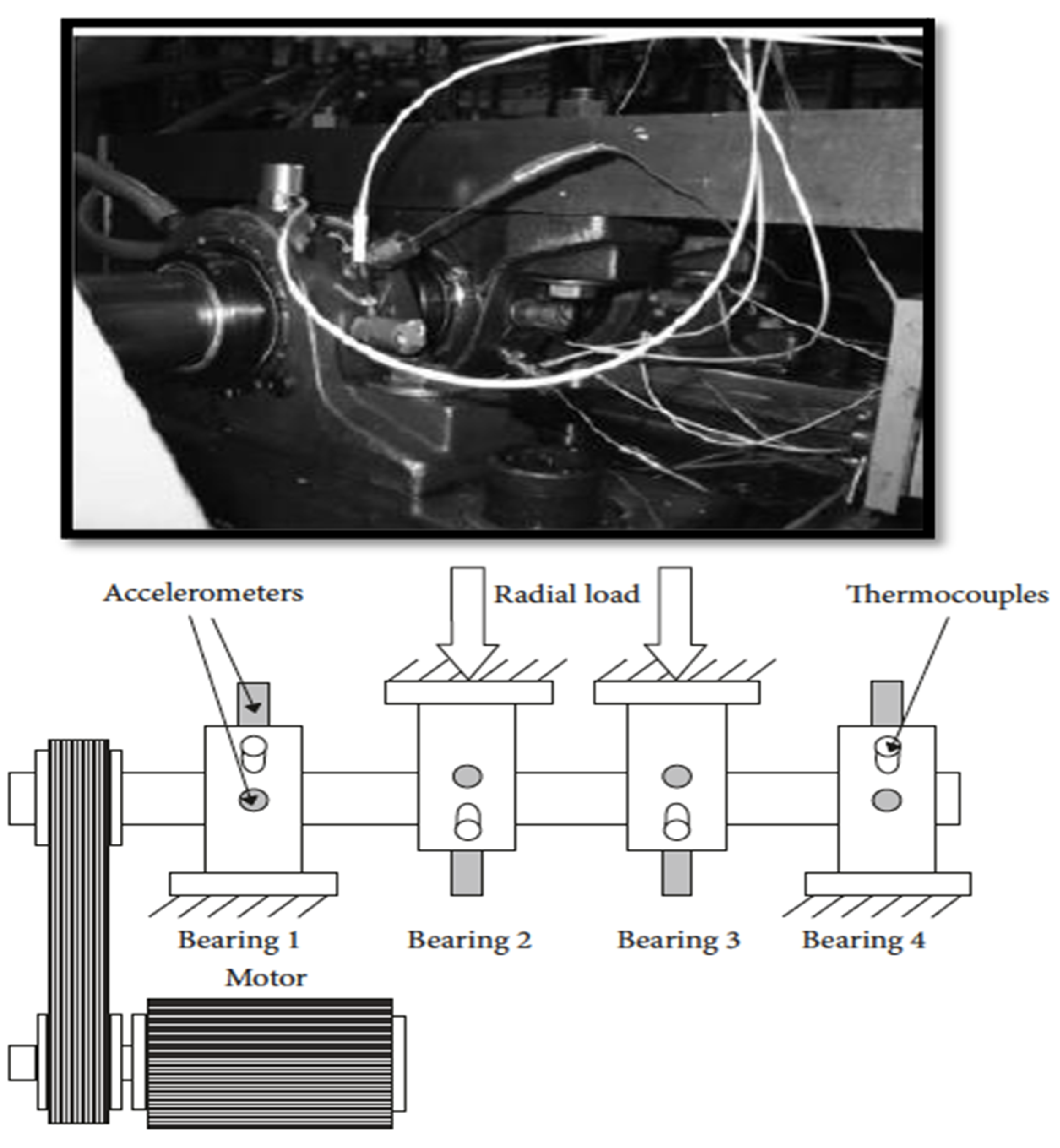
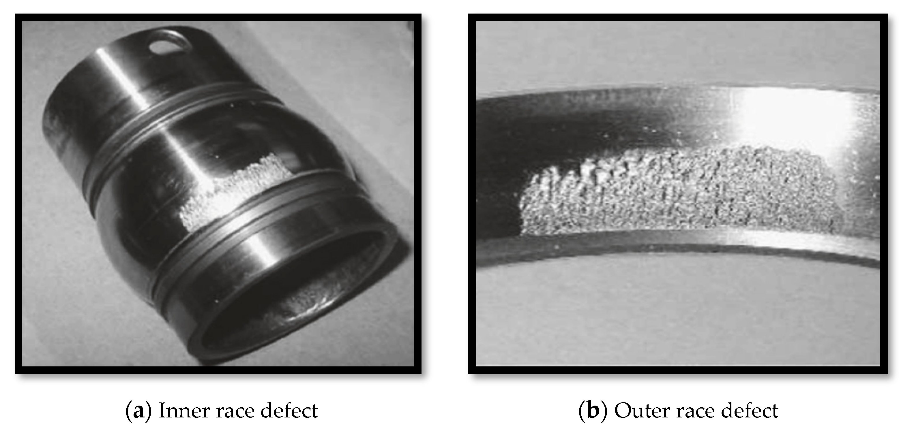
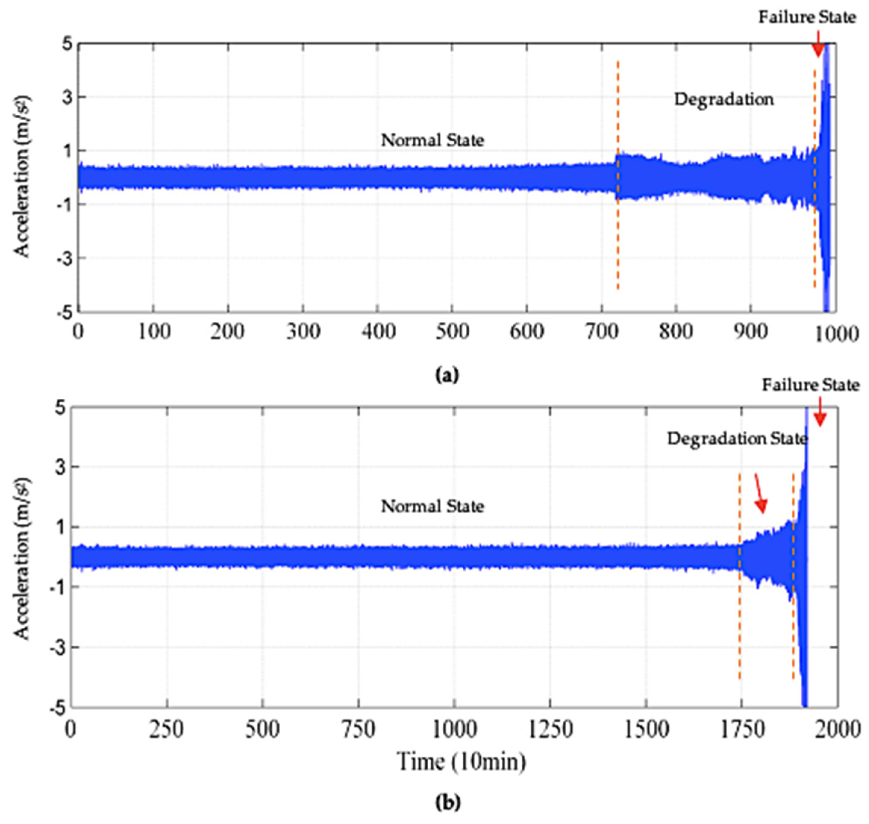
This section provides a detailed discussion of the dataset used, the experiments conducted, and the results.

3.1. Dataset

In this research study, we used the dataset from the Prognostic Data Repository of NASA, which was made publicly available by the Center of Intelligent Maintenance System (IMS), University of Cincinnati [44]. Details of the data acquired from the IMS database are in Table 1.

Table 1. Details of the dataset.

Type of Bearings	Double Rows Rexnord ZA-2115
No. of Bearings	Four (04)
Shaft Load	6000 lbs
Shaft Rotational Speed	2000 rpm
Type of Accelerometers	High Sensitivity Quartz ICP
No. of Accelerometers (Test 01)	Two (02) Accelerometers on x-axis and y-axis
No. of Accelerometers (Test 02 & Test 03)	One (01) Accelerometer
Sampling Rate	20 kHz

Figure 4 depicts the layout of the test rig. The data were collected for 1 s every 10 min. Each file has 20,480 data points, and the name of the file indicates the time at which the data was recorded. The test rig was lubricated using an oil circulation mechanism. The extent of debris stuck to a magnetic switch installed in the oil feedback pipe of the lubrication system indicated bearing degradation.

Figure 4. Test rig by IMS [44].

Figure 5a depicts Bearing 3 with an inner race fault at the end of the experiment recorded as Dataset 1. Figure 5b shows Bearing 1 with an outer race fault at the end of the experiment recorded as Dataset 2.

Figure 5. Physical condition of bearings after the run-to-failure experiment [45].

The plot of vibrational signals of bearing 1 in dataset 02 for the entire run-to-failure-experiment can be seen in Figure 6a. Whereas the plot of vibrational signals of bearing 3 in dataset 03 for the entire run-to-failure-experiment can be observed in Figure 6b. In Figure 6, the x-axis represents the time taken till the occurrence of a fault in the bearings, and the y-axis represents the vibration values recorded by the accelerometers in m/s².

Figure 6. Plot of Bearing Vibrational Signals after Run-to-Failure Experiment.

3.2. Experimental Setup

The dataset provided by IMS comprises three (03) datasets, each describing an independent run-to-failure experiment. Dataset 02, with a total of 984 files, was used for the training and testing of the model. The dataset was split into training and testing sets. 70% of the data was used for training the model, and 30% was used for testing. The results were further verified by testing the trained model using Dataset 03 with 4448 files.

At the end of run-to-failure experiments, in both Dataset 02 and Dataset 03, Bearing 1 and Bearing 3, respectively, developed an outer race fault. Therefore, the results were verified against Dataset 03 after performing the training and testing of the model on Dataset 02.

3.2.1. Data Pre-Processing

The data is first pre-processed to remove any outliers. After the data cleansing, it is then normalized. During normalization, the data is rescaled to fall between −1 and 1. The data is normalized using the min-max scaler function given in Equation (9).

$$x^{\prime }=\frac{x-\min \left(x\right)}{\max \left(x\right)-\min \left(x\right)}$$

(9)

where $x$ is the original value and $x^{\prime }$ is the normalized value.

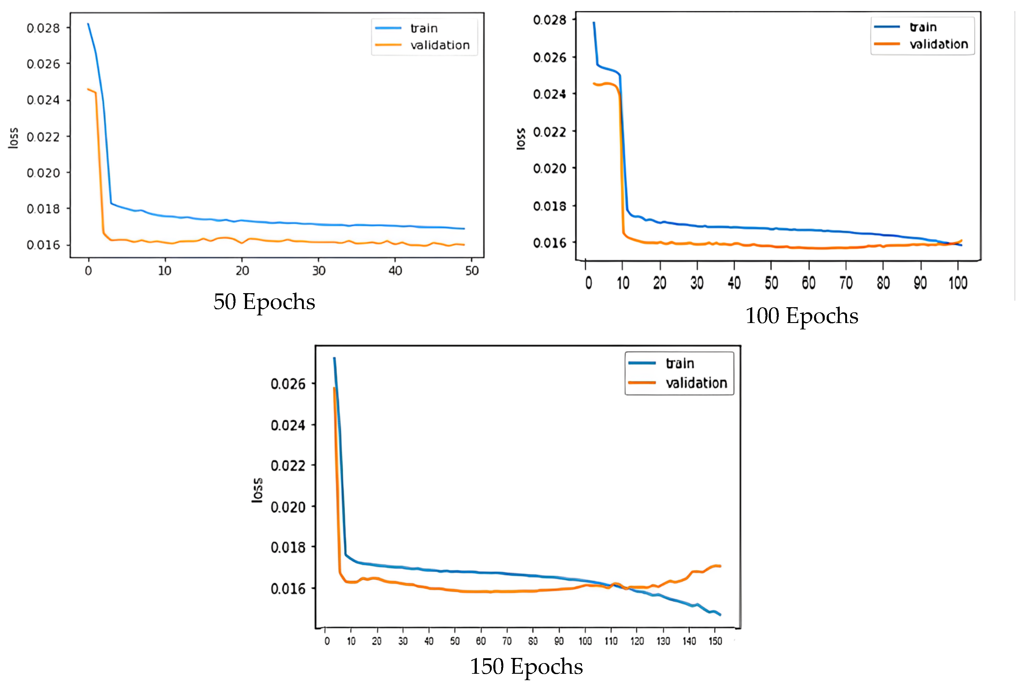
3.2.2. Hyper-Parameter Testing and Fine Tuning

During the fine-tuning and hyper-parameter testing, the model was trained for various epochs and the training and validation losses were calculated. Subsequently, the training and validation loss was plotted to visually analyze the model’s performance. Figure 7 depicts the training and validation loss for 50, 100, and 150 Epochs, respectively.

Figure 7. Training and Validation loss.

For 50 epochs, the graph depicts that the model is underfit since the validation and training plots do not converge. For 150 epochs, the model was getting overfit and could not be effectively generalized. The best-fit model was 100 epochs and a batch size of 50, whereas the sequence size had been set to 10.

The optimizer used for the model was ADAM. The reason for selecting Adam as an optimizer is that it has a learning rate of 0.001 by default. That is, it is neither too small nor too high and works best in the case of LSTM. A stacked LSTM model detailed in Table 2 was then defined.

Table 2. Characteristics of the LSTM model.

Type	Stacked LSTM
No. of Hidden Layers	Two (02)
No. of Memory Units	Layer 01: 128 Layer 02: 64
Optimizer	Adam
Batch Size	50
No. of Epochs	100

To make the model work effectively in real scenarios, all analyses were conducted on the actual time series data and in the time domain. Additionally, the cleansed data from the sensors were directly input into the model, contrary to other studies where either time–domain features or frequency–domain features were used as input to the model [37,38,39,40,41]. These statistical analyses and statistical feature extractions cannot be effectively carried out on partial data, especially in cases where prognostics are performed in real-time, and limited SCADA data is available at any time. Furthermore, LSTM has a competitive advantage where the need for feature engineering and extensive domain knowledge is minimized [43]. Hence, instead of extracting features, raw data from the sensors were directly input into the LSTM model.

3.3. Evaluation Metrics

The performance of the proposed methodology was evaluated using Root Mean Square Error (RMSE), Mean Absolute Error (MAE), Normalized Mean Absolute Error (NMAE), and Mean Absolute Percentage Error (MAPE) metrics given by Equations (10)–(13), respectively.

$$\mathrm{R}\mathrm{M}\mathrm{S}\mathrm{E}=\sqrt{\frac{1}{n}{\sum }_{i=1}^n{\left(y_i-{\widehat{y}}_i\right)}^2}$$

(10)

$$\mathrm{M}\mathrm{A}\mathrm{E}=\frac{1}{n}{\sum }_{i=1}^n{[y}_i-{\widehat{y}}_i]$$

(11)

$$\mathrm{N}\mathrm{M}\mathrm{A}\mathrm{E}=\frac{1}{n{\sigma }^2}{\sum }_{i=1}^n{{[y}_i-{\widehat{y}}_i]}^2$$

(12)

$$\mathrm{M}\mathrm{A}\mathrm{P}\mathrm{E}=\frac{1}{n}{\sum }_{i=1}^n{\left[\frac{y_i-{\widehat{y}}_i}{y_i}\right]}^2$$

(13)

$y_i$ denotes the actual values and ${\widehat{y}}_i$ denotes the predicted values. During the prognostics of bearing vibrational data, large errors can often result in undesirable outcomes. Because RMSE squares the difference between the actual and predicted values, it gives greater weight to the larger error values and hence is a very useful metric for the performance evaluation of the proposed model. Therefore, the comparison of the model with other similar research is carried out in terms of RMSE. However, to further verify and evaluate the performance of the model, MAE, NMAE, and MAPE have also been used as evaluation metrics.

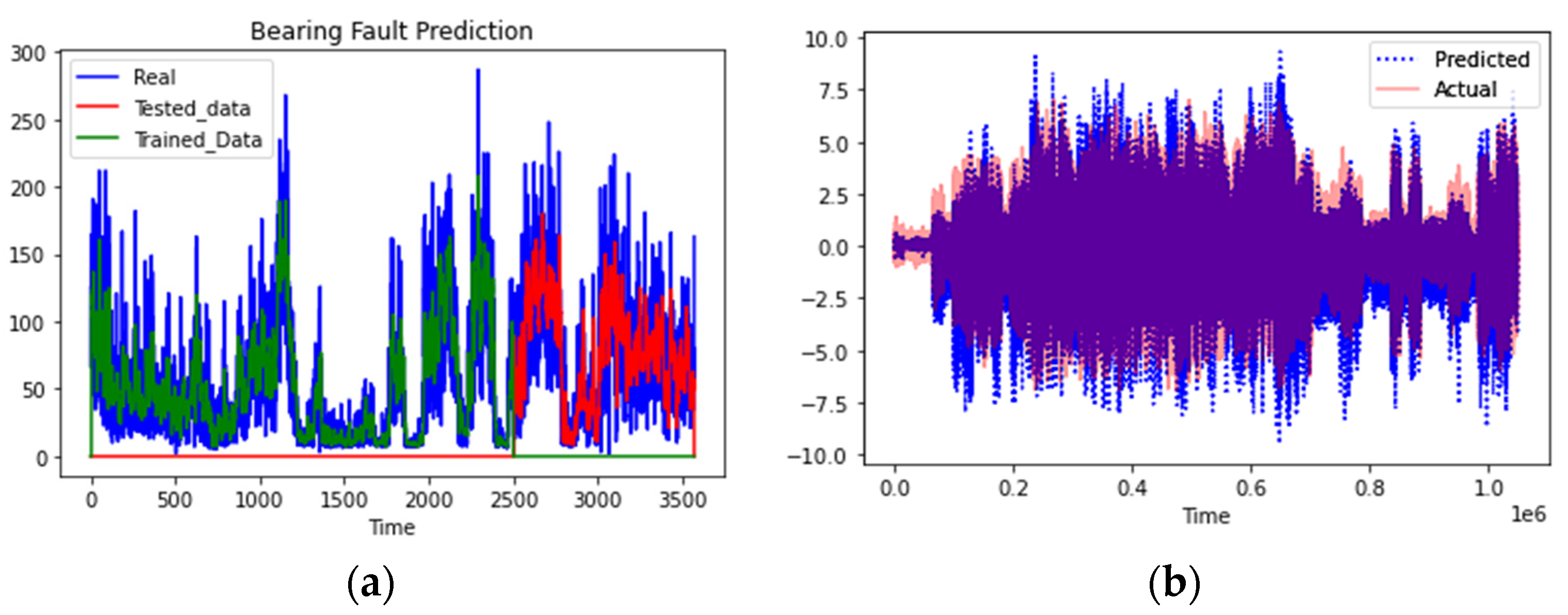
3.4. Results and Discussion

The performance of the developed LSTM model against the proposed approach was first analyzed on Dataset 02. Figure 8a shows the plot of the predicted and actual bearing vibration values. The blue color represents the actual bearing vibrations, whereas the orange color represents the predicted values. The proposed model precisely predicted the normal values and followed the degradation trend until a fault, which was also efficiently predicted. The RMSE value recorded for the Dataset 02 was 0.0145. Considering the mean vibration value, this RMSE reflects that the error in the predicted and actual values is less.

Figure 8. Plot of bearing vibrational signals—actual (blue) vs. predicted (orange) values.

The model’s performance was further verified by testing it against Dataset 03. Figure 8b depicts the predicted and actual values of the bearing vibrations. The model performed even better and achieved a remarkably low RMSE value of 0.0102. During the testing on Dataset 03, the model was also evaluated using MAE, NMAE, and MAPE. The error values in Table 3 reflect that the model performed extremely well while predicting the bearing vibration values.

Table 3. Model evaluation using various metrics.

Model	RMSE	MAE	NMAE	MAPE
LSTM using raw bearing vibration values	0.0102	0.0108	0.0002	0.0107

Removing noise in the frequency domain requires in-depth domain knowledge and can lead to the removal of significant data points that may prove useful for the model while analyzing patterns. Additionally, with LSTM, the requirement for extensive feature engineering is minimized, whereas when statistical time domain features are input into a model, they can add a biases factor, thereby affecting the prediction accuracy and limiting the generalization of the model. These issues have been efficiently addressed in this research.

The results achieved by the proposed model were then compared with similar research conducted on the IMS bearing dataset. Table 4 compares the RMSE of our research with the RMSE achieved by various models in other research that were trained and tested on the same dataset.

Table 4. Comparison of RMSE with similar research.

References	Year	Model	RMSE Value
Habbouche, H. et al. [34]	2021	LSTM Bi-LSTM	0.015 0.010
Lee, K. et al. [35]	2018	CNN Bi-LSTM Uni-LSTM	0.973
Berghout, T. et al. [36]	2021	LSTM	0.214
Akpudo et al. [37]	2020	Gaussian Process Regression (GPR) Deep Belief Network (DBN)	0.015 0.013
Yang et al. [40]	2020	LSTM DLSTM	0.030 0.010
Ding, H. et al. [46]	2020	LSTM	0.045
He, M. et al. [47]	2020	LSTM MRSVD-LSTM	0.025 0.012
Huang, G. et al. [48]	2020	MLSTM	0.766
Ge, Y. et al. [49]	2019	LSTM	0.020
Chen, Z. et al. [50]	2018	LSTM	0.109
Tang, G. et al. [51]	2018	LSTM	0.055
This Research	2023	LSTM	0.014 & 0.010

The researchers who achieved close RMSE values, such as [34], first extracted the time-frequency features from the data and then used those features as input to predict the future state of the bearings. However, in this research, for predicting the future vibration values, normalized raw vibration values of the bearings were used as input to the LSTM model. This not only helped reduce the need for feature engineering but also resulted in a better generalization of the model.

Table 5 compares the prediction accuracy of other machine learning and deep learning models with this research.

Table 5. Comparison of prediction accuracy with other machine learning models.

References	Classifier	Testing Accuracy
[52]	KNN	91.23%
[53]	SVM	62.5%
[54]	DNN with temporal coherence	94.9%
[55]	Compact 1D CNN	97.13%
This Research	LSTM using raw bearing vibration values	98.93%

The results reflect that our proposed methodology and model achieved better results in terms of RMSE than other research conducted on the same dataset. Also, the model developed in this research achieved better prediction accuracy than other deep learning and machine learning models when tested against the same dataset.

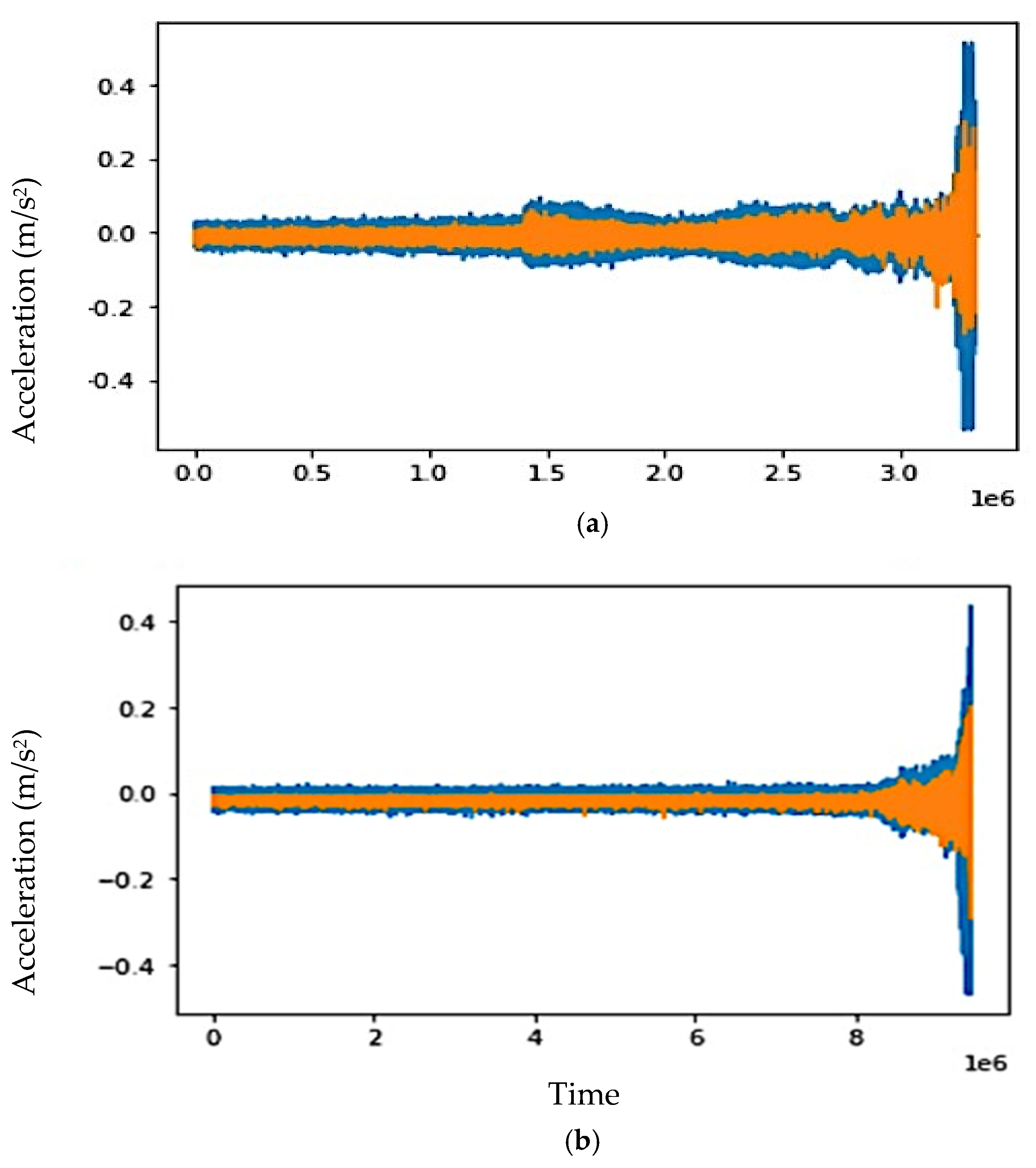
3.5. Generalization Capability of the Model

To evaluate the generalization capability of the model, it was tested against real vibration data generated by other electro-mechanical systems, including hydro and wind power turbines. The first set of bearing vibration data was acquired from the SCADA system installed at Neelum-Jehlum Hydro Power Project (NJHPP) Pakistan, having a total generation capacity of 969 MW. The second data set, publicly available [56], was acquired from a wind power project (WPP) operating in northern Sweden.

The plots depicted in Figure 9a,b again show that the model not only effectively predicted the bearing vibration values but also followed the trend in the data. Furthermore, a low RMSE value of 0.11 and 0.12 was recorded for the NJHPP and WPP datasets, respectively. The test results show that irrespective of the data source, the model can effectively predict the bearing vibration values.

Figure 9. Plot of Bearing Vibrational Signals—Actual vs. Predicted Values (NJHPP and WPP Datasets).

4. Conclusions

In lieu of the continual advancement of power generation units, the need to deploy efficient O&M procedures has increased. Hence, prognostics have become an important component of revolutionized electro-mechanical systems. Therefore, this research described an effective fault prognostics system for rolling element bearings based on univariate time series analysis using LSTM. The developed model was trained and tested using the bearings’ vibrational data. All analyses were conducted in the time domain, and raw sensor data was directly input into the model, thereby minimizing the need for feature engineering. The proposed approach was experimentally validated, and the model’s performance was analyzed in RMSE terms. The results were compared with other research conducted on the same dataset, and our model outperformed existing models and achieved a lower RMSE. The generalization capability of the model was verified by evaluating the performance of the model against real-time data generated by the SCADA system of a wind or hydropower turbine.

References

1. Kandukuri, S.T.; Klausen, A.; Karimi, H.R.; Robbersmyr, K.G. A review of diagnostics and prognostics of low-speed machinery towards wind turbine farm-level health management. Renew. Sustain. Energy Rev. 2016, 53, 697–708. [Google Scholar] [CrossRef]
2. Huang, B.; Di, Y.; Jin, C.; Lee, J. Review of data-driven prognostics and health management techniques: Lessons learned from PHM data challenge competitions. Mach. Fail. Prev. Technol. 2017, 2017, 1–17. [Google Scholar]
3. Yu, M.; Wang, D.; Luo, M. Model-based prognosis for hybrid systems with mode dependent degradation behaviors. IEEE Trans. Ind. Electron. 2014, 61, 546–554. [Google Scholar] [CrossRef]
4. Jardine, A.K.; Lin, D.; Banjevic, D. A review on machinery diagnostics and prognostics implementing condition-based maintenance. Mech. Syst. Signal Process. 2006, 20, 1483–1510. [Google Scholar] [CrossRef]
5. Govekar, E.; Gradišek, J.; Grabec, I. Analysis of acoustic emission signals and monitoring of machining processes. Ultrasonics 2000, 38, 598–603. [Google Scholar] [CrossRef]
6. Potočnik, P.; Govekar, E.; Grabec, I. Acoustic and acoustic emission based condition monitoring of production processes. In Proceedings of the Second World Congress on Asset Management and the Fourth International Conference on Condition Monitoring, Harrogate, UK, 11–14 June 2007; pp. 11–14. [Google Scholar]
7. Randall, R.B. Vibration-Based Condition Monitoring: Industrial, Aerospace and Automotive Applications; John Wiley & Sons: Hoboken, NJ, USA, 2011. [Google Scholar]
8. Ruiz-Cárcel, C.; Jaramillo, V.H.; Mba, D.; Ottewill, J.R.; Cao, Y. Combination of process and vibration data for improved condition monitoring of industrial systems working under variable operating conditions. Mech. Syst. Signal Process. 2016, 66, 699–714. [Google Scholar] [CrossRef]
9. Mohanty, A.R. Machinery Condition Monitoring: Principles and Practices; CRC Press: Boca Raton, FL, USA, 2014. [Google Scholar]
10. Lei, Y. Intelligent Fault Diagnosis and Remaining Useful Life Prediction of Rotating Machinery; Butterworth-Heinemann: Oxford, UK, 2016. [Google Scholar]
11. Rao, M.; Zuo, M.J. A new strategy for rotating machinery fault diagnosis under varying speed conditions based on deep neural networks and order tracking. In Proceedings of the 2018 17th IEEE International Conference on Machine Learning and Applications (ICMLA), Orlando, FL, USA, 17–20 December 2018; pp. 1214–1218. [Google Scholar]
12. Sarma, S.; Agrawal, V.; Udupa, S.; Parameswaran, K. Instantaneous angular position and speed measurement using a DSP based resolver-to-digital converter. Measurement 2008, 41, 788–796. [Google Scholar] [CrossRef]
13. Peeters, C.; Leclère, Q.; Antoni, J.; Lindahl, P.; Donnal, J.; Leeb, S.; Helsen, J. Review and comparison of tacholess instantaneous speed estimation methods on experimental vibration data. Mech. Syst. Signal Process. 2019, 129, 407–436. [Google Scholar] [CrossRef]
14. Zhang, X.; Zhao, B.; Lin, Y. Machine Learning Based Bearing Fault Diagnosis Using the Case Western Reserve University Data: A Review. IEEE Access 2021, 9, 155598–155608. [Google Scholar] [CrossRef]
15. Lei, Y.; Yang, B.; Jiang, X.; Jia, F.; Li, N.; Nandi, A.K. Applications of machine learning to machine fault diagnosis: A review and roadmap. Mech. Syst. Signal Process. 2020, 138, 106587. [Google Scholar] [CrossRef]
16. Fernandes, M.; Corchado, J.M.; Marreiros, G. Machine learning techniques applied to mechanical fault diagnosis and fault prognosis in the context of real industrial manufacturing use-cases: A systematic literature review. Appl. Intell. 2022, 52, 14246–14280. [Google Scholar] [CrossRef] [PubMed]
17. Iatsenko, D.; McClintock, P.V.; Stefanovska, A. Extraction of instantaneous frequencies from ridges in time–frequency representations of signals. Signal Process. 2016, 125, 290–303. [Google Scholar] [CrossRef]
18. Dziedziech, K.; Jablonski, A.; Dworakowski, Z. A novel method for speed recovery from vibration signal under highly non-stationary conditions. Measurement 2018, 128, 13–22. [Google Scholar] [CrossRef]
19. Schmidt, S.; Heyns, P.S.; De Villiers, J.P. A tacholess order tracking methodology based on a probabilistic approach to incorporate angular acceleration information into the maxima tracking process. Mech. Syst. Signal Process. 2018, 100, 630–646. [Google Scholar] [CrossRef]
20. Khan, N.A.; Jönsson, P.; Sandsten, M. Performance comparison of time-frequency distributions for estimation of instantaneous frequency of heart rate variability signals. Appl. Sci. 2017, 7, 221. [Google Scholar] [CrossRef]
21. Urbanek, J.; Barszcz, T.; Sawalhi, N.; Randall, R.B. Comparison of amplitude-based and phase-based method for speed tracking in application to wind turbines. Metrol. Meas. Syst. 2011, 18, 295–303. [Google Scholar] [CrossRef]
22. Urbanek, J.; Barszcz, T.; Antoni, J. A two-step procedure for estimation of instantaneous rotational speed with large fluctuations. Mech. Syst. Signal Process. 2013, 38, 96–102. [Google Scholar] [CrossRef]
23. Cardona-Morales, O.; Avendaño, L.; Castellanos-Dominguez, G. Nonlinear model for condition monitoring of non-stationary vibration signals in ship driveline application. Mech. Syst. Signal Process. 2014, 44, 134–148. [Google Scholar] [CrossRef]
24. LeCun, Y.; Bengio, Y.; Hinton, G. Deep learning. Nature 2015, 521, 436–444. [Google Scholar] [CrossRef]
25. Jia, F.; Lei, Y.; Lin, J.; Zhou, X.; Lu, N. Deep neural networks: A promising tool for fault characteristic mining and intelligent diagnosis of rotating machinery with massive data. Mech. Syst. Signal Process. 2016, 72, 303–315. [Google Scholar] [CrossRef]
26. Ali, M.Z.; Shabbir, M.N.S.K.; Liang, X.; Zhang, Y.; Hu, T. Machine Learning-Based Fault Diagnosis for Single- and Multi-Faults in Induction Motors Using Measured Stator Currents and Vibration Signals. IEEE Trans. Ind. Appl. 2019, 55, 2378–2391. [Google Scholar] [CrossRef]
27. Khalid, S.; Lim, W.; Kim, H.S.; Oh, Y.T.; Youn, B.D.; Kim, H.-S.; Bae, Y.-C. Intelligent Steam Power Plant Boiler Waterwall Tube Leakage Detection via Machine Learning-Based Optimal Sensor Selection. Sensors 2020, 20, 6356. [Google Scholar] [CrossRef] [PubMed]
28. Ma, M.; Sun, C.; Chen, X. Discriminative deep belief networks with ant colony optimization for health status assessment of machine. IEEE Trans. Instrum. Meas. 2017, 66, 3115–3125. [Google Scholar] [CrossRef]
29. Afridi, Y.S.; Ahmad, K.; Hassan, L. Artificial intelligence based prognostic maintenance of renewable energy systems: A review of techniques, challenges, and future research directions. Int. J. Energy Res. 2022, 46, 21619–21642. [Google Scholar] [CrossRef]
30. He, M.; He, D. Deep Learning Based Approach for Bearing Fault Diagnosis. IEEE Trans. Ind. Appl. 2017, 53, 3057–3065. [Google Scholar] [CrossRef]
31. Zhuang, L.; Xu, A.; Wang, X.-L. A prognostic driven predictive maintenance framework based on Bayesian deep learning. Reliab. Eng. Syst. Saf. 2023, 234, 109181. [Google Scholar] [CrossRef]
32. Jagatheesaperumal, S.K.; Rahouti, M.; Ahmad, K.; Al-Fuqaha, A.; Guizani, M. The Duo of Artificial Intelligence and Big Data for Industry 4.0: Review of Applications, Techniques, Challenges, and Future Research Directions. arXiv 2021, arXiv:2104.02425. [Google Scholar] [CrossRef]
33. Khan, A.; Hwang, H.; Kim, H.S. Synthetic Data Augmentation and Deep Learning for the Fault Diagnosis of Rotating Machines. Mathematics 2021, 9, 2336. [Google Scholar] [CrossRef]
34. Habbouche, H.; Benkedjouh, T.; Zerhouni, N. Intelligent prognostics of bearings based on bidirectional long short-term memory and wavelet packet decomposition. Int. J. Adv. Manuf. Technol. 2021, 114, 145–157. [Google Scholar] [CrossRef]
35. Lee, K.; Kim, J.K.; Kim, J.; Hur, K.; Kim, H. Stacked convolutional bidirectional LSTM recurrent neural network for bearing anomaly detection in rotating machinery diagnostics. In Proceedings of the 2018 1st IEEE International Conference on Knowledge Innovation and Invention (ICKII), Jeju, Republic of Korea, 23–27 July 2018; pp. 98–101. [Google Scholar]
36. Berghout, T.; Benbouzid, M.; Mouss, L.H. Leveraging Label Information in a Knowledge-Driven Approach for Rolling-Element Bearings Remaining Useful Life Prediction. Energies 2021, 14, 2163. [Google Scholar] [CrossRef]
37. Akpudo, U.E.; Hur, J.-W. Towards bearing failure prognostics: A practical comparison between data-driven methods for industrial applications. J. Mech. Sci. Technol. 2020, 34, 4161–4172. [Google Scholar] [CrossRef]
38. Akpudo, U.E.; Hur, J.-W. A feature fusion-based prognostics approach for rolling element bearings. J. Mech. Sci. Technol. 2020, 34, 4025–4035. [Google Scholar] [CrossRef]
39. Ali, J.B.; Fnaiech, N.; Saidi, L.; Chebel-Morello, B.; Fnaiech, F. Application of empirical mode decomposition and artificial neural network for automatic bearing fault diagnosis based on vibration signals. Appl. Acoust. 2015, 89, 16–27. [Google Scholar]
40. Yang, C.; Ma, J.; Wang, X.; Li, X.; Li, Z.; Luo, T. A novel based-performance degradation indicator RUL prediction model and its application in rolling bearing. ISA Trans. 2021, 121, 349–364. [Google Scholar] [CrossRef]
41. Wu, H.; Huang, A.; Sutherland, J.W. Avoiding Environmental Consequences of Equipment Failure via an LSTM-Based Model for Predictive Maintenance. Procedia Manuf. 2020, 43, 666–673. [Google Scholar] [CrossRef]
42. Sherstinsky, A. Fundamentals of recurrent neural network (RNN) and long short-term memory (LSTM) network. Phys. D Nonlinear Phenom. 2020, 404, 132306. [Google Scholar] [CrossRef]
43. Hochreiter, S.; Schmidhuber, J. Long short-term memory. Neural Comput. 1997, 9, 1735–1780. [Google Scholar] [CrossRef]
44. Lee, J.; Qiu, H.; Yu, G.; Lin, J. Rexnord Technical Services, “Bearing Data Set”. In IMS, University of Cincinnati. NASA Ames Prognostics Data Repository; NASA Ames: Moffett Field, CA, USA, 2007. Available online: https://ti.arc.nasa.gov/tech/dash/groups/pcoe/prognostic-data-repository/ (accessed on 18 July 2021).
45. Qiu, H.; Lee, J.; Lin, J.; Yu, G. Wavelet filter-based weak signature detection method and its application on rolling element bearing prognostics. J. Sound Vib. 2006, 289, 1066–1090. [Google Scholar] [CrossRef]
46. Ding, H.; Yang, L.; Cheng, Z.; Yang, Z. A remaining useful life prediction method for bearing based on deep neural networks. Measurement 2021, 172, 108878. [Google Scholar] [CrossRef]
47. He, M.; Zhou, Y.; Li, Y.; Wu, G.; Tang, G. Long short-term memory network with multi-resolution singular value decomposition for prediction of bearing performance degradation. Measurement 2020, 156, 107582. [Google Scholar] [CrossRef]
48. Huang, G.; Li, H.; Ou, J.; Zhang, Y.; Zhang, M. A reliable prognosis approach for degradation evaluation of rolling bearing using MCLSTM. Sensors 2020, 20, 1864. [Google Scholar] [CrossRef] [PubMed]
49. Ge, Y.; Guo, L.; Dou, Y. Remaining useful life prediction of machinery based on KS distance and LSTM neural network. Int. J. Perform. Eng. 2019, 15, 895. [Google Scholar]
50. Chen, Z.; Liu, Y.; Liu, S. Mechanical state prediction based on LSTM neural network. In Proceedings of the 2017 36th Chinese Control Conference (CCC), Dalian, China, 26–28 July 2017; pp. 3876–3881. [Google Scholar]
51. Tang, G.; Zhou, Y.; Wang, H.; Li, G. Prediction of bearing performance degradation with bottleneck feature based on LSTM network. In Proceedings of the 2018 IEEE International Instrumentation and Measurement Technology Conference (I2MTC), Houston, TX, USA, 14–17 May 2018; pp. 1–6. [Google Scholar]
52. Yaqub, M.F.; Gondal, I.; Kamruzzaman, J. Inchoate Fault Detection Framework: Adaptive Selection of Wavelet Nodes and Cumulant Orders. IEEE Trans. Instrum. Meas. 2012, 61, 685–695. [Google Scholar] [CrossRef]
53. Hu, Q.; He, Z.; Zhang, Z.; Zi, Y. Fault diagnosis of rotating machinery based on improved wavelet package transform and SVMs ensemble. Mech. Syst. Signal Process. 2007, 21, 688–705. [Google Scholar] [CrossRef]
54. Zhang, R.; Peng, Z.; Wu, L.; Yao, B.; Guan, Y. Fault diagnosis from raw sensor data using deep neural networks considering temporal coherence. Sensors 2017, 17, 549. [Google Scholar] [CrossRef]
55. Eren, L.; Ince, T.; Kiranyaz, S. A generic intelligent bearing fault diagnosis system using compact adaptive 1D CNN classifier. J. Signal Process. Syst. 2018, 91, 179–189. [Google Scholar] [CrossRef]
56. Wind Power Project, Gearbox Bearing Vibration Dataset. Available online: http://urn.kb.se/resolve?urn=urn:nbn:se:ltu:diva-70730 (accessed on 15 January 2023).
Disclaimer/Publisher’s Note: The statements, opinions and data contained in all publications are solely those of the individual author(s) and contributor(s) and not of MDPI and/or the editor(s). MDPI and/or the editor(s) disclaim responsibility for any injury to people or property resulting from any ideas, methods, instructions or products referred to in the content.
Article Metrics
Citations
Article Access Statistics
Multiple requests from the same IP address are counted as one view.