Abstract
In order to realize robot-assisted spinal laminectomy surgery and meet the clinical needs of the robot workspace, including accuracy in human–robot collaboration, an asymmetrical 3-DOF spatial translational robot is proposed, which can realize spinal laminectomy in a fixed posture. First, based on the screw theory, the constraint screw system of the robot was established, and the degree of freedom was derived to verify the spatial translational ability of the robot. Then, a kinematic model of the robot was established, and a static force model of the robot was derived based on the kinematic model. The mathematical relationship between the external force and the joint force/torque was obtained, with the quality of all links considered in the model. Finally, we modeled the robot and imported it into ADAMS to obtain the static force simulation results of the 3D model. The force error was approximately 0.001 N and the torque error was approximately 0.0001 N∙m compared with the simulation results of the mathematical model, accounting for 1% of the joint force/torque, which is acceptable. The result also showed the correctness of the mathematical models, and provides a theoretical basis for motion control and human–robot collaboration.
1. Introduction
With the increasing trend of the aging of the population in China, spinal diseases are becoming a main complaint in clinic [1,2,3]. Percutaneous pedicle screw fixation with the assistance of intraoperative image navigation [4,5] or surgical robots [6,7] is relatively mature. There are not many results for robot-assisted laminectomy, although related research has been carried out previously [8,9,10].
In a robot-assisted surgery system, considering the needs of clinical surgery, the robot needs to be able to achieve three-dimensional space translation in a fixed posture. Most of the existing 3-DOF parallel mechanisms [11,12,13] adopted symmetrical structures to make the workspace symmetrical. However, from the perspective of the anatomical size of the spine, due to the smaller size of the lamina in the coronal plane and the larger distance from the skin surface, the existing symmetrical parallel structure cannot meet laminectomy requirements under the requirements of the workspace and the volume of the mechanism. Because of low stiffness and accuracy, the serial mechanism is also not competent for milling with contact force. Therefore, an asymmetric structure 3-DOF parallel robot is proposed in this paper. The robot is partially decoupled such that the motion in the coronal plane would not be affected by motion in the perpendicular direction to the coronal plane.
During the surgery, in order to avoid the interference of robots with patients and instruments and to give surgeons the maximum autonomy, the robot is required to have the ability of human–robot collaboration. There are two ways to achieve human–robot collaboration. One method is to consider the robot as a virtual system [14,15,16], which requires a force sensor. This would increase the difficulty of disinfection when the force sensor is placed at the end of the robot, and it would also affect the overall stiffness of the robot when the force sensor is placed at the joints. The cost of the system may also increase while using force sensors. Therefore, this method is not suitable for laminectomy surgery. Another method is to establish a nonlinear mathematical model of the joint force, joint position and end force of the robot by using the force balance method [17] to realize human–robot collaboration. This model is mostly established by the introduction of dynamics [18], and is suitable for situations in which the robot moves quickly and the acceleration changes frequently. However, in the process of robot-assisted surgery, the speed is low and gentle, so a static force model can meet the needs. In this paper, a method based on force balance was used to realize human–robot collaboration [19,20]. In addition, a new force sensing model [21,22,23] was referenced in the establishment of the static force model of the asymmetrical parallel robot, and the precision and efficiency could be guaranteed by the force sensing model.
In order to realize accurate control of the robot, first, the degree of freedom of the robot was analyzed based on the screw theory, and then the kinematic model analysis and static force analysis were carried out. After the models were established, simulation results of the asymmetrical 3-DOF parallel robot were obtained to verify the correctness of the kinematic model and the static force model.
2. Methods
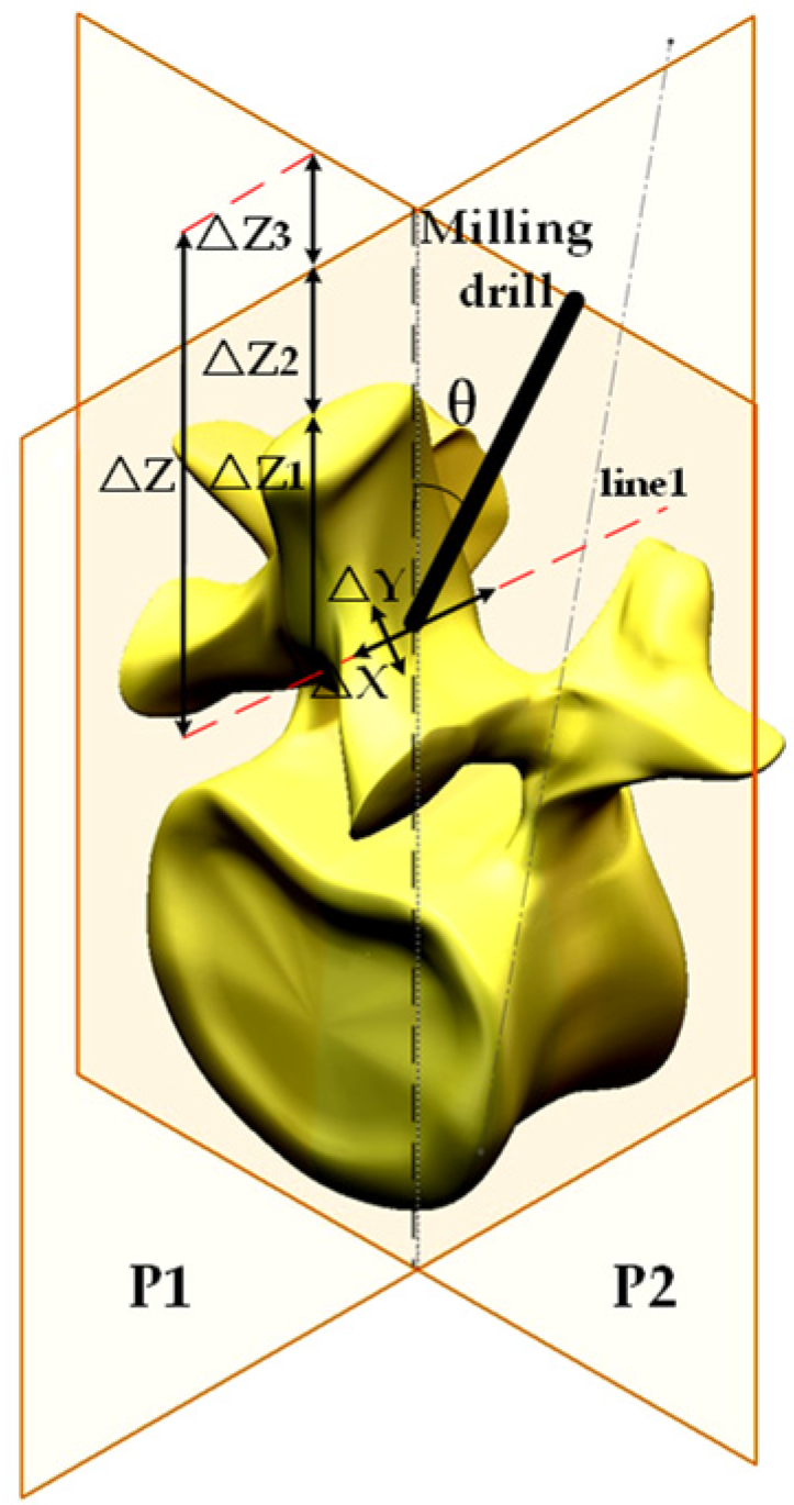
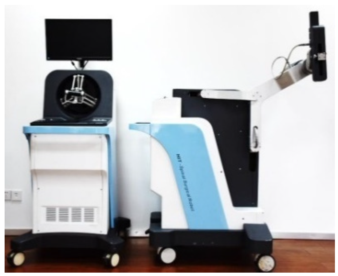
In laminectomy, we need to control the milling drill moving in a fixed posture along the line1 trajectory, which is shown in Figure 1. However, in order to avoid interference with bone tissue during the milling process, it is necessary to make a milling drill with an angle and surface P1. In fact, the proposed robot would first be installed at the end of a 5-DOF hybrid manipulator by fast switching [24]; a hybrid manipulator would then be used to achieve the initial positioning at pose , and then the proposed robot would be used to achieve the milling at a fixed pose. The hybrid manipulator is shown in Figure 2; it is not the focus of this paper and does not require much discussion.

Figure 1.
Anatomic size of human vertebra segment.
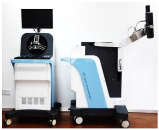
Figure 2.
5-DOF hybrid manipulator.
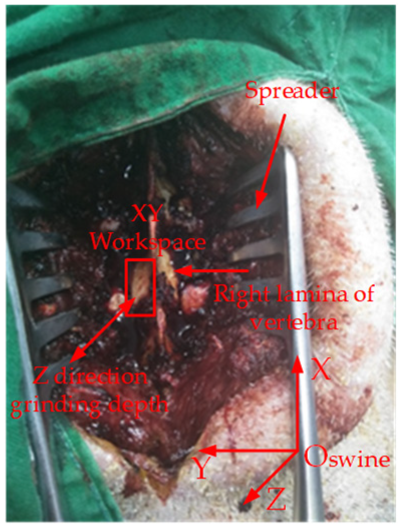
Clinically, spinal laminectomy usually requires complete exposure of the lamina to the surgeon’s field of vision under the assistance of a spreader, as shown in Figure 3. It can be observed from Figure 3 that the anatomical size of the swine lamina in the x and y directions of the coordinate system is significantly smaller than the distance from the lamina along the z direction to the skin surface.

Figure 3.
Swine spinal laminectomy surgery.
The anatomical size of human spine is different from that of swine, and is shown in Figure 1. mm, mm, mm, where is the length of the lamina spinous process, is the thickness of fat (the distance from the spinous process to the skin surface), is the safe distance required between the milling drill and the human skin surface before grinding. The anatomical size obtained above is the requirement for the workspace of the robot.
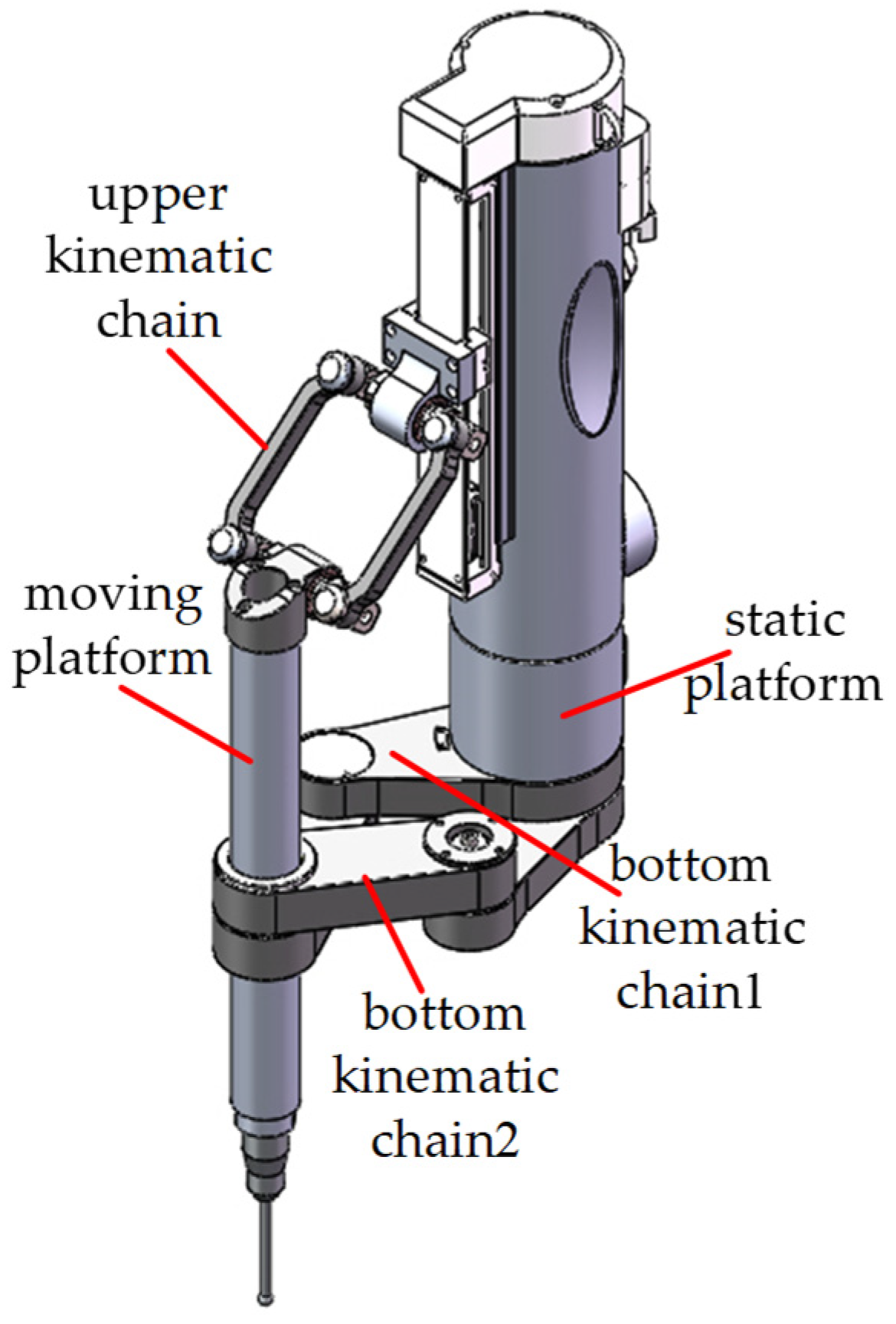
Based on the analysis above, it is difficult for a parallel robot with a symmetrical structure to meet the needs of laminectomy considering the workspace and robot volume. To solve this problem, a 3-DOF space translational robot with an asymmetrical structure is proposed in this paper. As shown in Figure 4, the robot consists of one upper kinematic chain, two bottom kinematic chains, a static platform and a moving platform.

Figure 4.
Asymmetrical 3-DOF parallel robot.
2.1. Degree of Freedom Analysis Based on Screw Theory
The first task in designing a new robot is analyzing the degrees of freedom to further achieve accurate motion control. It can be seen from Figure 4 that the upper kinematic chain contains a parallelogram mechanism. In order to facilitate the analysis of the degrees of freedom, we simplified the upper kinematic chain and replaced the parallelogram with a generalized kinematic pair [25]. The kinematic sketch of the robot is shown in Figure 5.
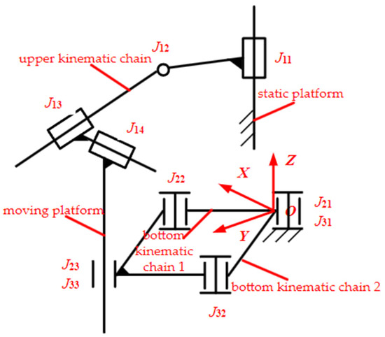
Figure 5.
Kinematic sketch of robot.
As seen in Figure 5, the upper chain is driven by a translation joint , and consists of a generalized revolution joint and two generalized translation joints and . Bottom kinematic chains 1 and 2 adopt symmetrical structures, which are driven by the revolution joint (), and consist of the revolution joint () and cylinder joint (). The degree of freedom of the proposed robot is derived via screw theory. The classical DoF calculation formula, named the Kutzbach–Grübler formula, can be expressed as:
where n is the number of links, g is the number of kinematic joints, and is the number of degrees of freedom of the i-th kinematic joint. Equation (1) can obtain correct results for traditional simple mechanisms, but it is unsuitable for complex spatial mechanisms, mainly due to the existence of the common constraint and the redundant constraint. Therefore, a modified Kutzbach–Grübler equation is expressed as:
where d is the order of the mechanism, v is the redundant constraint, and is the local degree of freedom. The order and redundant constraint of the mechanism need to be obtained based on the screw theory, while the local degree of freedom can be obtained by observation.
First, we obtained the kinematic screw of each joint based on the screw theory, such that the screw system of three kinematic chains is established as:
where a1, b1, a2, b2, a3, b3, a4, b4, a5, b5, a6, b6 are different real values which would change with the motion of each joint of the robot. The constraint screw of each chain could be computed by Equation (3) and the property that the reciprocal product of the constraint screw and the kinematic screw is zero, and expressed as:
When the reciprocal product is computed by a constraint spinor and all kinematic spinors of the robot are zero, the constraint spinor is considered a common constraint. Therefore, according to Equation (4), a common torque constraint around the Y axis of the robot could be obtained:
According to Equation (4), each chain has another constraint in addition to the public constraint, and the three constraints are linearly correlated, i.e., there is also a redundant constraint. Therefore, according to Equation (2), the degree of freedom of the robot can be derived as:
In addition, according to Equation (4), each chain contains only a torque constraint without a force constraint on the moving platform. Thus, we can conclude that the robot could achieve translation movement in 3D space.
2.2. Kinematic Model Analysis
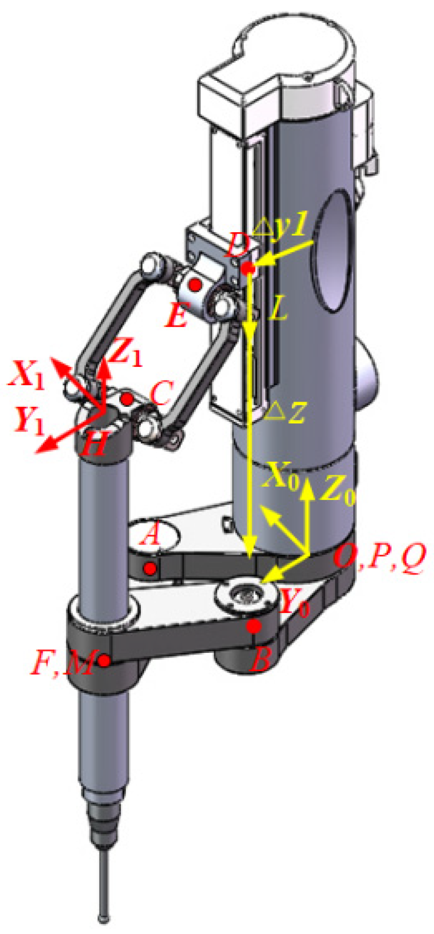
The base coordinate system O-X0Y0Z0 and the end coordinate system H-X1Y1Z1 were established on the robot, as shown in Figure 6. The distance of the initial position of point D in Y direction of the base coordinate system was set as , the distance in Z direction was set as , the length of link DE was set as , the length of link EC was set as , the length of link CH was set as , the control value of upper kinematic active joint was set as L, and the coordinate of point H was set as . Then, the position coordinates of points D, E, C could be derived as , , and , respectively. Finally, the kinematic equation of the upper chain was established based on the length of link EC:

Figure 6.
Coordinate system of kinematic model.
For the bottom kinematic chain, let the length of links OA, OB, AF, BM be lOA = lOB and lAF = lBM, let be the angle between OA and the X positive axis of the base coordinate, and let be the angle between OB and the X positive axis of the base coordinate. Then, we can obtain the position coordinates of point A and B as and , respectively. The position coordinates of point F and point M are . Finally, based on the length of the links AF and BM, the kinematic equations of the two bottom chains are established as:
Using Equations (7) and (8), the robot kinematic model could be obtained as:
2.3. Static Force Model Analysis
Based on the kinematic model, the mathematical model of joint force/torque and external load could be obtained by analyzing the force of the upper chain, bottom chain 1, bottom chain 2 and moving platform.
2.3.1. Force Analysis of Upper Kinematic Chain
(1) Force analysis of passive link EC
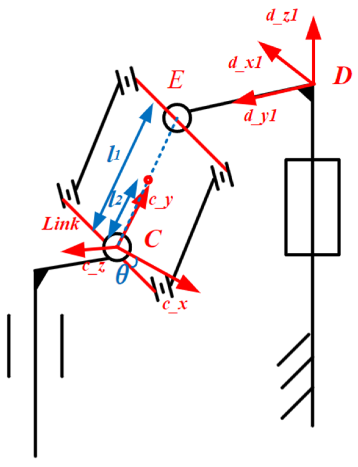
The upper chain contains a passive parallelogram mechanism, which is considered link EC for convenience. We first established a coordinate system at point C. The c_y axis is from C to E along the link. The c_z axis is obtained by cross-multiplication of the c_y axis and the parallelogram transverse link. The c_x axis is determined by the right-hand rule, as shown in Figure 7. The coordinate could be expressed as:
where
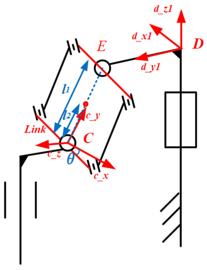
Figure 7.
Coordinate system of the upper kinematic chain.
According to the characteristics of passive parallelogram motion, the c_z axis is equivalent to a revolution joint for points C and E. Thus, the torque on points C and E to the c_z axis is zero, i.e.,:
Assume that the angle between the c_x axis and the horizontal link of the passive parallelogram is . Since the horizontal link and the moving platform are connected by a revolution joint, the torque of point C to the direction of the horizontal link is zero. Similarly, the results at point E are as follows:
In addition, let the gravity of link EC be , so that the projection on the base coordinate is:
According to Equation (10), we can derive the projection of the gravity of link EC in the C coordinates as:
where
Let the projections of force and torque on points C and E in the C coordinates be:
The spatial equilibrium equation of EC at the origin of the C coordinate system are listed as follows:
According to Equations (11), (12) and (17), the force analysis of passive link EC could be obtained as:
where and are the distances from point E and the center of gravity to the origin of the C coordinates along the c_y axis, respectively.
(2) Force analysis of active link DE
We established a coordinate system at point D. The d_y1 axis is from D to E along the link direction. The d_x1 axis is obtained by multiplying the d_y1 axis by the Z axis of the base coordinates. The d_z1 axis is obtained by the right-hand rule, as shown in Figure 7. The coordinate could be expressed as:
The gravity of active link DE is projected in the base coordinate system as:
According to Equation (19), we can obtain the projection of gravity of DE in coordinate system D as:
The force of link EC on link DE at point E is the same as that of link DE on link EC at point E in the opposite direction. Therefore, we can conclude:
According to Equation (10), we can obtain the transformation matrix of coordinate C in the base coordinates:
Then, the projection of in the base coordinates is:
According to Equation (19), the projection of in the D coordinates could be further computed as:
i.e.,:
The force balance equation of active link DE in the d_z1 axis direction of the origin column of the D coordinates is:
where f is the driving force. Using Equations (18) and (27), the force of the moving platform on link CE at point C could be obtained as follows:
where
According to the law of action force and reaction force, the force of link CE on the moving platform at point C could be obtained as:
According to Equation (23), we can obtain the projection of in the base coordinates:
2.3.2. Force Analysis of Bottom Kinematic Chain 1
(1) Force Analysis of bottom kinematic chain 1
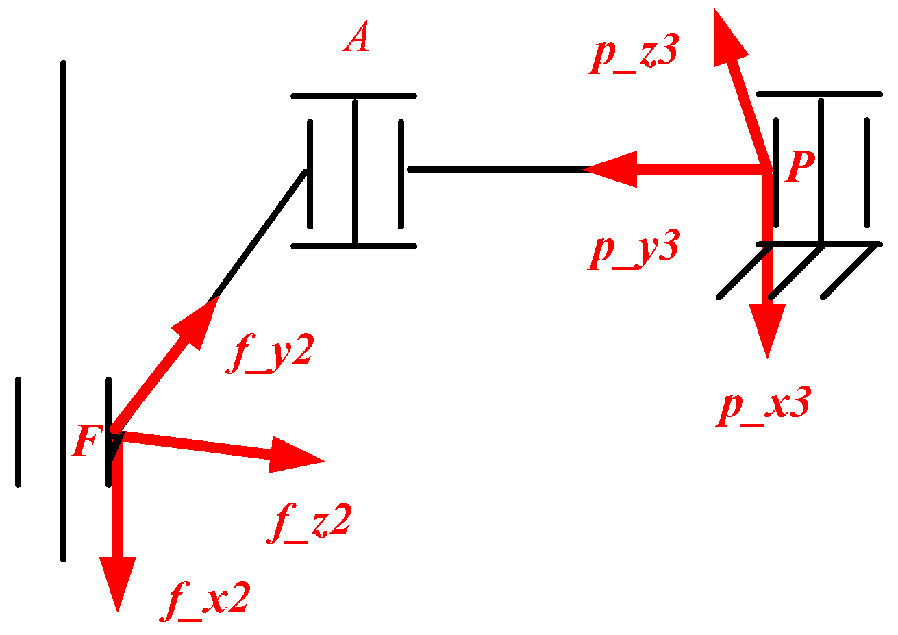
We established a coordinate system at point F. The f_y2 axis points to A along the direction of the link. The f_z2 axis is obtained by cross-multiplying the f_y2 axis with the Z axis of the base coordinate system. The f_x2 axis is obtained by the right-hand rule, as shown in Figure 8.
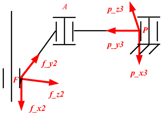
Figure 8.
Coordinate system of bottom kinematic chain 1.
The F coordinates can be expressed as:
where
The robot is a cylindrical joint at point F, so the force and torque on point F in the direction of the f_x2 axis are both zero, and the torque on point A in the direction of the f_x2 axis is also zero, which can be expressed as:
The projection of AF’s gravity in the base coordinate system is as follows:
According to Equation (31), we can obtain the projection of AF’s gravity in coordinate system F as:
where
Let the projection of force and torque on point F in the F coordinates be
and the projection of force and torque on point A in the F coordinates be
The spatial equilibrium equation of passive link AF at the origin of the F coordinates is expressed as:
where is the distance of point A to the origin of the F coordinates along the f_y2 axis and is the distance between the center of gravity of link AF and the origin of the F coordinates along the f_y2 axis. According to Equations (32) and (37), the force analysis of bottom kinematic chain 1 could be obtained as:
(2) Force Analysis of Active Link PA
We established a coordinate system at point P. The p_y3 axis points from P to A along the link direction. The p_z3 axis is obtained by cross-multiplication of the p_y3 axis and the Z axis of the base coordinate system. The p_x3 is determined by the right-hand rule. As shown in Figure 8, the coordinate system at point P could also be expressed as:
where
The projection of link PA’s gravity on the base coordinate system is:
From Equation (39), we can obtain the projection of PA’s gravity in coordinate system P:
where
We also know that the force of link FA on link AP is a pair of interaction force of link AP on link AF, so we obtain:
According to Equation (31), we can obtain the transformation matrix between the coordinate F and the base coordinates:
Then, the projection of force on the base coordinates is:
Furthermore, we can find the projection of force in the P coordinates:
Then we obtain:
The space torque balance equation of AP along p_x3 axis in the P coordinates is:
where is the distance from point A to point P along the link, and is the distance from the center of gravity of link AP to point P. Using Equation (47), we could obtain:
where
T1 is the driving torque of bottom kinematic chain 1. At point F, there is a pair of interaction force between link AF and moving platform AF, so we obtain:
Using Equation (43), we obtain the projection of in the base coordinates as:
2.3.3. Force Analysis of Bottom Kinematic Chain 2
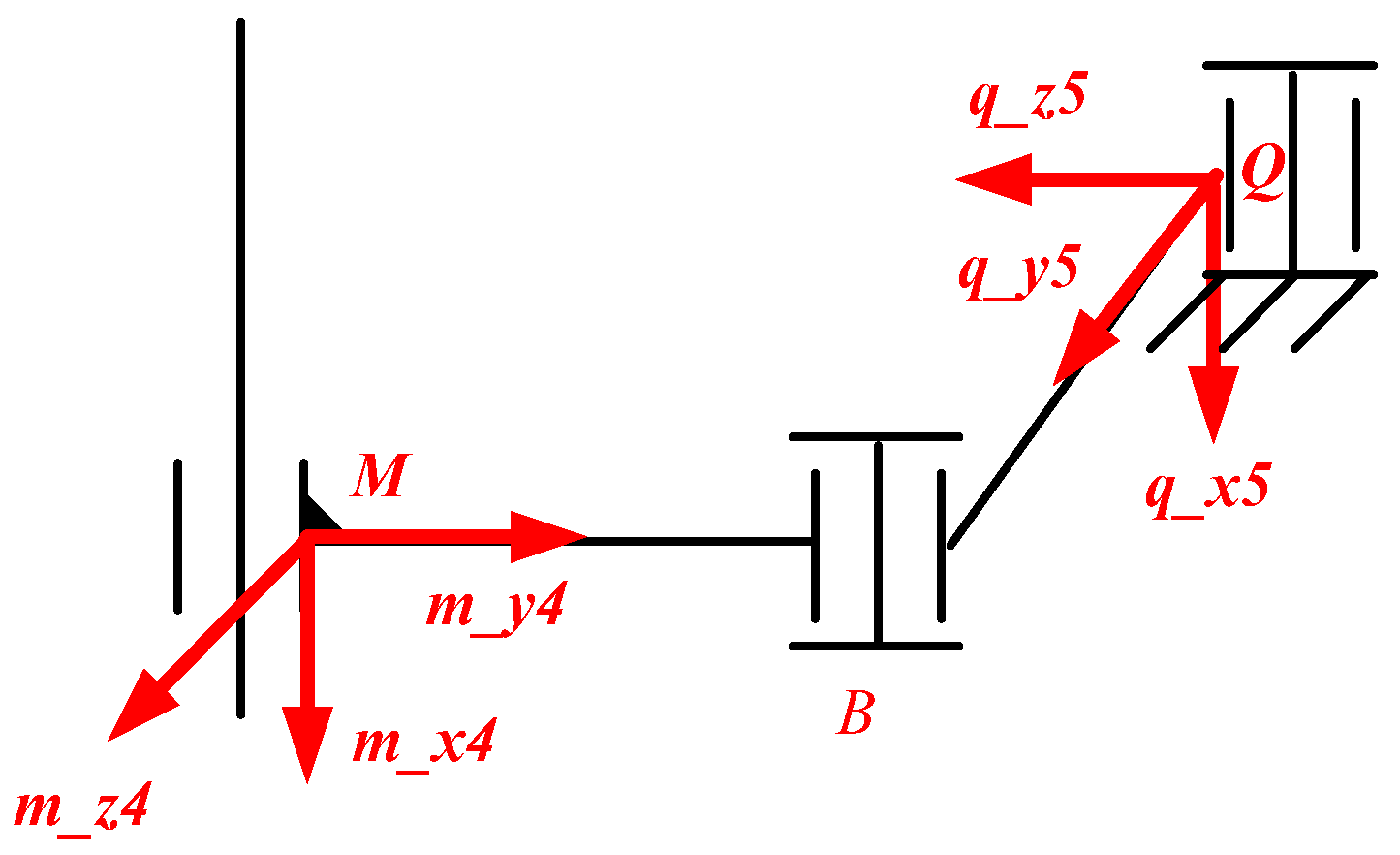
The analysis method of bottom kinematic chain 2 is similar to the way we analyzed bottom kinematic chain 1. The force analysis coordinate system is established as shown in Figure 9, and we directly give the projection of the force of bottom kinematic chain 2 to the moving platform in the base coordinate system as:

Figure 9.
Coordinate system of bottom kinematic chain 2.
2.3.4. Force Analysis of the Moving Platform
The force of each kinematic chain on the moving platform in the base coordinate system was obtained in the previous part. Next, considering the case of load, the force balance equation of the moving platform is expressed as:
where is the external load of the moving platform and is the gravity of the moving platform projected to the base coordinate system. Equation (52) reflects the relationship between the joint driving force/torque and the external load. Without considering external load, the model reflects the joint force/torque required to resist the gravity of all links at different positions.
3. Simulation and Result Analysis
Through the previous mathematical modeling, we obtained the mathematical model of the relationship between the external load and joint force/torque. It can also be seen from the model that Equation (52) could be considered a gravity compensation model when the load is set as zero. In order to verify the correctness of the static force model, we used ADAMS software to realize a 3D model simulation and compare the simulation results with the mathematical model simulation using MATLAB. The correctness of the mathematical model was evaluated using the calculated error percentage of the joint force/torque.
We adopted Solidworks software to realize the 3D modeling of the robot and measure the relevant parameters in the static force model, as shown in Table 1. In order to fully demonstrate the correctness of the mathematical model, we took five sets of simulation experiments, as shown in Table 2.

Table 1.
Parameters of static model.

Table 2.
Parameters of simulations.
Table 2 includes five sets of simulations corresponding to the external load and the driving angle/position range. The main difference between Simulation 1 and the others was the external load. Simulation 1 set the load in all three directions to zero to verify the correctness of the gravity compensation model. In simulations 2, 3, 4, and 5, the forces on the three axes of the base coordinate system were not zero, which was used to verify the correctness of the mathematical model of load force and joint force/torque. Note that in the simulation process using ADAMS, quasi-static simulation was mainly realized by continuous slow motion, while the MATLAB simulation was realized by selecting discrete points within the range of joint motion.
We imported the 3D model into ADAMS and added the kinematic joint according to the actual constraints of the robot. In practice, it is difficult to add the constraints of all components accurately. Therefore, in order to simplify the simulation’s complexity without affecting the accuracy of static force simulation, we simplified the structure of the robot by removing screws, caps and so on, which are small in both volume and mass. The imported 3D model in ADAMS is shown in Figure 10.
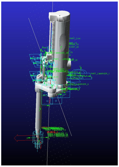
Figure 10.
3D model in ADAMS.
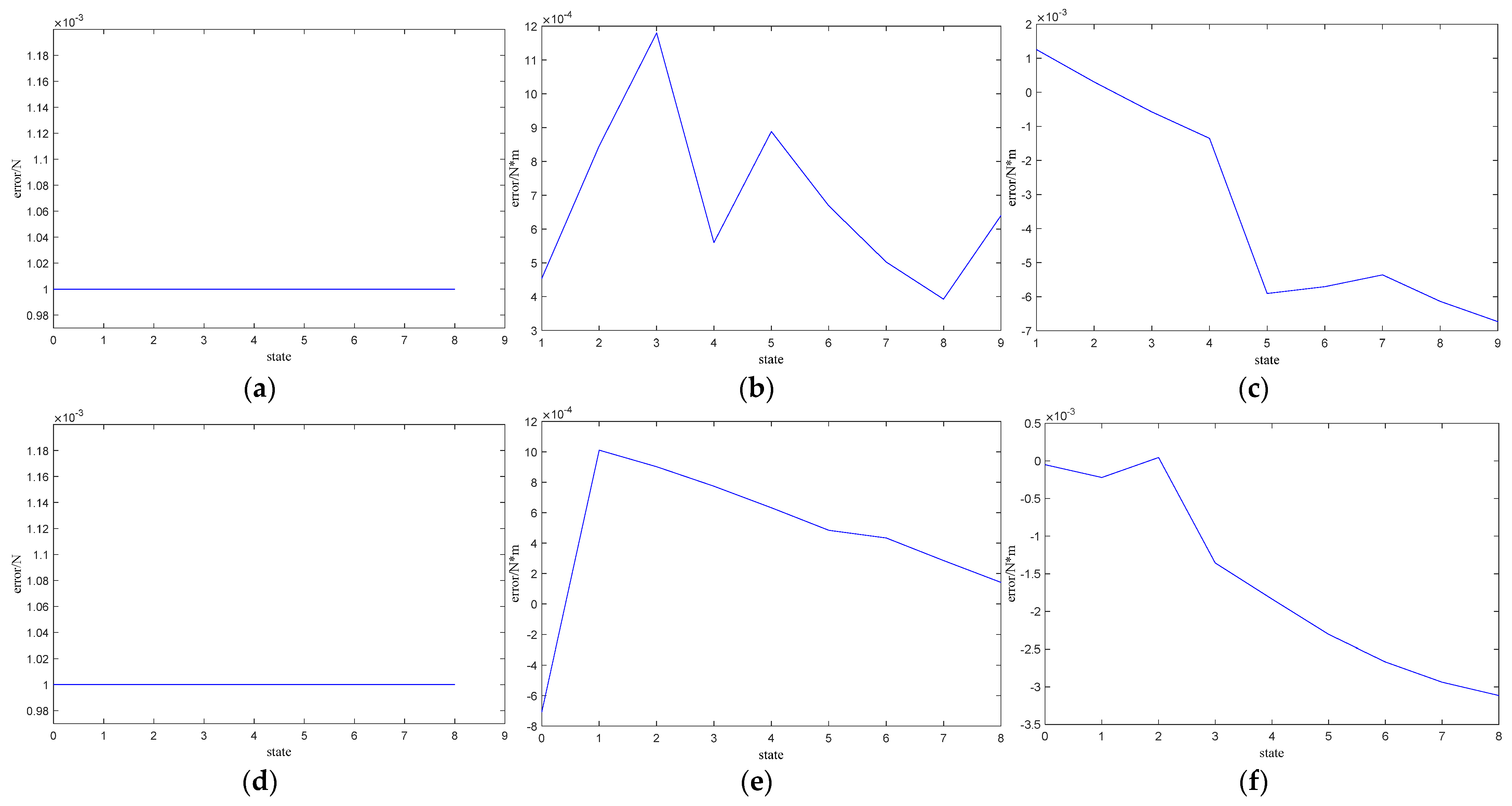
After ADAMS simulation according to the parameters of Simulation 1 in Table 2, the simulation results were compared with those from the mathematical model using MATLAB with the same simulation parameters, whose results are shown in Figure 11. Figure 11a shows the force curve of the upper kinematic chain driving joint in the simulation process, and Figure 11b,c show the torque curves of the bottom kinematic chains 1 and 2 driving joints in the simulation process, respectively. As shown in Figure 11, when the load is zero, the simulation curve of the mathematical model basically coincides with that of the 3D model. In order to further observe the error variance, we defined the difference between the mathematical model simulation results and the 3D model simulation results as error, and computed the error of each kinematic chain, as shown in Figure 12. Figure 12a shows the error of the upper kinematic chain, Figure 12b shows the error of bottom kinematic chain 1 and Figure 12c shows the error of bottom kinematic chain 2.

Figure 11.
Comparison results of simulation 1. (a) Upper kinematic chain; (b) Bottom kinematic chain 1; (c) Bottom kinematic chain 2.

Figure 12.
Error of simulation 1. (a) Upper kinematic chain. (b) Bottom kinematic chain 1. (c) Bottom kinematic chain 2.
It can be seen from Figure 12 that the magnitude of output error is 0.001 N, and the magnitude of torque error is 0.0001 N∙M. The influence of error on the actual force/torque can be more intuitively observed by considering the error as a percentage. Therefore, we used Equation (53) to compute the percentage of error in the joint force/torque. The error was approximately 1%, and therefore can be ignored, which also verifies the correctness of the static force model. According to detailed analysis, the simulation error was mainly composed of two parts. One was the error introduced by parameters measured in Solidworks, and the other was the quasi-static simulation after importing to ADAMS, which also brought error.
where is the force/torque obtained by 3D model simulation and is the force/torque obtained by mathematical model simulation.
Similar to the process of Simulation 1, according to the parameters of Simulation 2 in Table 2, simulation was carried out in ADAMS and compared with the simulation results of the MATLAB mathematical model. The results are shown in Figure 13.

Figure 13.
Comparison results of simulation 2. (a) Upper kinematic chain. (b) Bottom kinematic chain 1. (c) Bottom kinematic chain 2.
It can be seen from Figure 13 that the mathematical model and the simulation curve of the 3D model were basically coincident under the condition of external load. The error curve is shown in Figure 14. Equation (53) was again used to compute the error, accounting for approximately 1% of the joint force/torque, and the error could be ignored. The causes of error were the same as in Simulation 1.

Figure 14.
Error of simulation 2. (a) Upper kinematic chain. (b) Bottom kinematic chain 1. (c) Bottom kinematic chain 2.
The error curves of Simulations 3, 4, 5 are shown in Figure 15, and the correctness of the static force model could be further verified. It is noticed that the error obtained by Equation (53) could be larger than 1% when the joint force/torque was smaller than 0.01 N/0.01 N∙m. The reason is that percentage error is more susceptible to smaller joint force/torque. In fact, this case could be solved by setting a small threshold for joint driving.
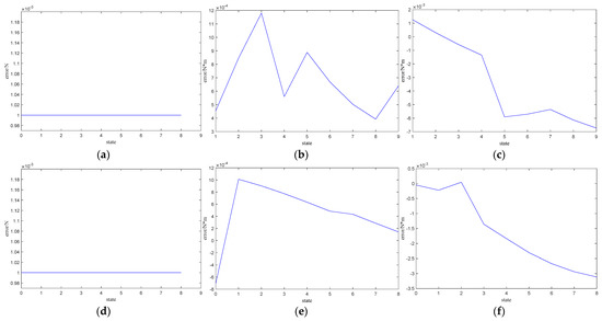

Figure 15.
Errors of simulation 3, simulation 4 and simulation 5. (a) Upper chain in simulation 3. (b) Bottom chain 1 in simulation 3. (c) Bottom chain 2 in simulation 3. (d) Upper chain in simulation 4. (e) Bottom chain 1 in simulation 4. (f) Bottom chain 2 in simulation 4. (g) Upper chain in simulation 5. (h) Bottom chain 1 in simulation 5. (i) Bottom chain 2 in simulation 5.
The error obtained from the above five sets of simulation experiments accounted for approximately 1% of the joint force/torque, i.e., the static mathematical model was acceptable. Simulation 1 verified the gravity compensation model, and Simulations 2, 3, 4, and 5 verified the mathematical relationship between the external load and the joint force/torque. In addition, it should be emphasized that the kinematic model was involved in the derivation of the static mathematical model, so the correctness of the kinematic model was indirectly verified through the simulation of the static model.
4. Conclusions
In this paper, a spinal vertebral lamina milling robot with three-dimensional translational motion is proposed. First, the constraints of the robot were analyzed using screw theory, and then the degree of freedom of the robot is derived. Then, a kinematic model of the robot was established. Based on the kinematic analysis, we derived a static model of the robot and established the relationship between the load force and the joint force/torque. Finally, we used five sets of data to simulate and compare the 3D model and the mathematical model. The comparison error accounted for approximately 1% of the joint force/torque, and the accuracy was acceptable, which also verified the correctness of the kinematic model and the static model. However, the static force model was established in this paper by considering only the mass of all links. In actual working conditions, friction and other factors would affect both gravity compensation and force sensing. Therefore, the problem mentioned above is the task to be further studied in the next stage.
Author Contributions
Conceptualization, S.L. and P.G.; methodology, S.L.; software, S.L.; validation, S.L., P.G. and H.Y.; formal analysis, H.Y.; investigation, M.C.; resources, P.G.; data curation, S.L.; writing—original draft preparation, S.L.; writing—review and editing, P.G. All authors have read and agreed to the published version of the manuscript.
Funding
This research received no external funding.
Institutional Review Board Statement
Not applicable.
Data Availability Statement
Not applicable.
Conflicts of Interest
The authors declare no conflict of interest.
References
- Kumar, M. Global, regional, and national burden of traumatic brain injury and spinal cord injury, 1990–2016: A systematic analysis for the Global Burden of Disease Study 2016. Lancet Neurol. 2018, 18, 107–116. [Google Scholar]
- Yang, S.; Yu, Y.; Ji, Y.; Luo, D.J.; Zhang, Z.Y.; Huang, G.P.; He, F.Y.; Wu, W.J.; Mou, X.P. Multi-drug resistant spinal tuberculosis-epidemiological characteristics of in-patients: A multicentre retrospective study. Epidemiol. Infect. 2020, 148. [Google Scholar] [CrossRef] [PubMed] [Green Version]
- Zhang, H.R.; Qiao, R.Q.; Yang, X.G.; Hu, Y.C. A multicenter, descriptive epidemiologic survey of the clinical features of spinal metastatic disease in China. Neurol. Res. 2020, 42, 11. [Google Scholar] [CrossRef] [PubMed]
- Ttorsten, J.; Sprengel, K.; Peterer, L.; Mica, L.; Werner, C.M.L. 3D navigation of endoscopic rhizotomy at the lumlink spine. J. Clin. Neurosci. 2016, 23, 101–105. [Google Scholar] [CrossRef]
- Linkrigo, N.; Gernot, L.; Lian, X.; Berlin, C.; Janssen, I.; Jada, A.; Alimi, M.; Härtl, R. Total Navigation in Spine Surgery; A Concise Guide to Eliminate Fluoroscopy Using a Portable Intraoperative Computed Tomography 3-Dimensional Navigation System. World Neurosurg. 2017, 100, 325–335. [Google Scholar]
- Lonjon, N.; Chan-Seng, E.; Costalat, V.; Bonnafoux, B.; Vassal, M.; Boetto, J. Robot-assisted spine surgery: Feasibility study through a prospective case-matched analysis. Eur. Spine J. 2016, 25, 947–955. [Google Scholar] [CrossRef]
- Laratta, J.L.; Shillingford, J.N.; Lombardi, J.M.; Alrabaa, R.G.; Benkli, B.; Fischer, C.; Lenke, L.G.; Lehman, R.A. Accuracy of S2 Alar-Iliac Screw Placement Under Robotic Guidance. Spine Deform. 2018, 6, 130–136. [Google Scholar] [CrossRef] [PubMed]
- Wang, T.; Luan, S.; Hu, L.; Liu, Z.; Li, W.; Jiang, L. Force-based control of a compact spinal milling robot. Int. J. Med. Robot. Comput. Assist. Surg. 2010, 6, 178–185. [Google Scholar] [CrossRef] [PubMed]
- Deng, Z.; Jin, H.; Hu, Y.; He, Y.; Zhang, P.; Tian, W.; Zhang, J. Fuzzy Force Control and State Detection in Vertebral Lamina Milling. Mechatronics 2016, 35, 1–10. [Google Scholar] [CrossRef]
- Luan, S.; Wang, T.; Li, W.; Liu, Z.; Jiang, L.; Hu, L. 3D navigation and monitoring for spinal milling operation based on registration between multiplanar fluoroscopy and CT images. Comput. Methods Programs Biomed. 2012, 108, 151–157. [Google Scholar] [CrossRef]
- Zhang, C.; Li, B.; Zhao, X. Kinematics and working performance analysis of a 3-DOF parallel mechanism. Manuf. Autom. 2017, 39, 54–58. [Google Scholar]
- Liu, X.; Wang, J.; Pritschow, G. A new family of spatial 3-DOF fully-parallel manipulators with high rotational capability. Mech. Mach. Theory 2005, 40, 475–494. [Google Scholar] [CrossRef]
- Stan, S.; Manic, M.; Szep, C.; Balan, R. Performance analysis of 3 DOF Delta parallel robot. In Proceedings of the International Conference on Human System Interactions, Yokohama, Japan, 19–21 May 2011; pp. 215–220. [Google Scholar]
- Lecours, A.; Mayer, B.; Gosselin, C. Variable admittance control of a four-degree-of-freedom intelligent assist device. In Proceedings of the International Conference on Robotics & Automation, St Paul, MN, USA, 14–18 May 2012; pp. 3903–3908. [Google Scholar]
- Mao, D.; Yang, W.; Du, Z. Fuzzy variable impedance control based on stiffness identification for human-robot cooperation. In Proceedings of the IOP Conference Series: Earth and Environmental Science, Chengdu, China, 26–28 May 2017. [Google Scholar]
- Dimeas, F.; Aspragathos, N. Reinforcement learning of variable admittance control for human-robot co-manipulation. In Proceedings of the IEEE/RSJ International Conference on Intelligent Robots & Systems, Hamburg, Germany, 28 September–2 October 2015; pp. 1011–1016. [Google Scholar]
- Park, C.; Kyung, J.H.; Do, H.M.; Choi, T. Development of direct teaching robot system. In Proceedings of the 2011 8th International Conference on Ubiquitous Robots and Ambient Intelligence (URAI), Incheon, Korea, 23–26 November 2011; pp. 730–732. [Google Scholar]
- Hou, C.; Wang, Z.; Zhao, Y.; Song, G. Load Adaptive Force-free Control for the Direct Teaching of Robots. Robot 2017, 39, 439–448. [Google Scholar]
- You, Y.; Zhang, Y.; Li, C. Force-free Control for the Direct Teaching of Robots. J. Mech. Eng. 2014, 50, 10–17. [Google Scholar] [CrossRef]
- Wang, H.; Du, Z.; Yan, Z.; Liu, R. Gravity Compensation Algorithm for Hybrid Master Manipulator. Robot 2014, 36, 111–116. [Google Scholar]
- Yu, L.; Song, H.; Wang, T.; Wang, Z.; Sun, L.; Du, Z. A new asymmetrical mass distribution method on the analysis of universal “force-sensing” model for 3-DOF translational parallel manipulator. Ind. Robot Int. J. 2014, 41, 56–69. [Google Scholar] [CrossRef]
- Sun, L.; Yu, L.; Du, Z. Static analysis on new force sensing system of 6-DOF parallel robot. J. Harbin Inst. Technol. 2004, 36, 1030–1033. [Google Scholar]
- Yu, L.; Zhang, N.; Zhang, L.; Wang, D. A SimMechanics simulation of static forces in a 3-RPS parallel robot. J. Harbin Eng. Univ. 2010, 31, 1061–1064. [Google Scholar]
- Peng, Y.; Yu, H.; Du, Z. Design and Kinematic Analysis of a Hybrid Manipulator for Spine Surgery. In Proceedings of the IEEE/International Conference on Mechatronics and Automation, Harbin, China, 7–10 August 2016; pp. 884–889. [Google Scholar]
- Huang, Z.; Zhao, Y.; Zhao, T. Advanced Spatial Mechanism; Advanced Education Press: Beijing, China, 2006; pp. 115–138. [Google Scholar]
Publisher’s Note: MDPI stays neutral with regard to jurisdictional claims in published maps and institutional affiliations. |
© 2022 by the authors. Licensee MDPI, Basel, Switzerland. This article is an open access article distributed under the terms and conditions of the Creative Commons Attribution (CC BY) license (https://creativecommons.org/licenses/by/4.0/).

