Yukawa Potential, Panharmonic Measure and Brownian Motion

Abstract

This paper continues our earlier investigation, where a walk-on-spheres (WOS) algorithm for Monte Carlo simulation of the solutions of the Yukawa and the Helmholtz partial differential equations (PDEs) was developed by using the Duffin correspondence. In this paper, we investigate the foundations behind the algorithm for the case of the Yukawa PDE. We study the panharmonic measure, which is a generalization of the harmonic measure for the Yukawa PDE. We show that there are natural stochastic definitions for the panharmonic measure in terms of the Brownian motion and that the harmonic and the panharmonic measures are all mutually equivalent. Furthermore, we calculate their Radon–Nikodym derivatives explicitly for some balls, which is a key result behind the WOS algorithm.

1. Introduction and Preliminaries

The harmonic measure is a fundamental tool in geometric function theory, and it has interesting applications in the study of bounded analytic functions, quasiconformal mappings and potential theory. For example, the harmonic measure has proven very useful in the study of quasidisks and related topics (see, e.g., [1,2,3]). Results involving the harmonic measure have been given by numerous authors since the 1930s (see [4] and references therein). In this paper, we consider the panharmonic measure, which is a natural counterpart of the classical harmonic measure, whereby the harmonic functions related are replaced with the smooth solutions to the Yukawa equation:

$$\Delta u\left(x\right)={\mu }^{2}u\left(x\right),{\mu }^2\ge 0.$$

(1)

Equation (1) first arose from the work of the Japanese physicist Hideki Yukawa in particle physics. Here, $u:D\to \mathbb{R}$ is a two-times differentiable function and $D\subset {\mathbb{R}}^n$, $n\ge 2$ is a domain. The Yukawa equation was first studied in order to describe the nuclear potential of a point charge. This model led to the concept of the Yukawa potential (also called a screened Coulomb potential), which satisfies an equation of the type given by Equation (1). The Yukawa equation also arises from certain problems related to optics (see [5]). Clearly, when $\mu =0$, we have the Laplace equation, and, indeed, the results given in this paper reduce to the classical results.

Using the terminology of Duffin [6,7], we call a function $u:D\to \mathbb{R}$ panharmonic, or μ-panharmonic, in a domain D if its second derivatives are continuous and if it satisfies the Yukawa equation (Equation (1)) for all $x\in D$. The function u is called panharmonic at $x_0\in D$ if there is a neighborhood of $x_0$ where u is panharmonic.

In Definition 1 of the panharmonic measure below, and in all that follows, we always assume that $n\ge 2$, although some results are also true in the dimension $n=1$. For Definition 1, we need the notions of smallness and the regularity of a domain. These are best given by using the stochastic characterization via the Brownian motion. We refer to any of the classical textbooks [8,9,10] for further details.

We recall that the n-dimensional Brownian motion $W=\left(W\right(t);t\ge 0)$ starting from the point $x\in {\mathbb{R}}^n$ is the time-homogeneous Markov process with the Markov semigroup

$$P\left(t\right)f\left(x\right)={\mathbb{E}}^x\left[f\left(W\left(t\right)\right)\right]$$

given by

$$P\left(t\right)=e^{t\frac{1}{2}\Delta };$$

that is, $\frac{1}{2}\Delta$ is the generator of the Markov semigroup of the Brownian motion.

A domain $D\subset {\mathbb{R}}^n$ is regular if the Brownian motion does not dwell on its boundary; more precisely, D is (Wiener) regular if

$${\mathbb{P}}^x\left[{\tau }_D=0\right]=1,\mathrm{for}\mathrm{all}x\in \partial D,$$

where ${\mathbb{P}}^x$ is the probability measure under which ${\mathbb{P}}^x[W\left(0\right)=x]=1$, and

$${\tau }_D=inf\left\{t>0;W\left(t\right)\in D^c\right\}$$

is the first hitting time of the Brownian motion in the set $D^c$. We call a regular domain D (Wiener) small if a Brownian motion starting inside D eventually will leave the domain; that is, D is small if

$${\mathbb{P}}^x\left[{\tau }_D<\infty \right]=1,\mathrm{for}\mathrm{all}x\in D.$$

For example, all bounded domains are small. All half-spaces are also small.

The panharmonic, or $\mu$-panharmonic, measure is a generalization of the harmonic measure:

Definition 1.

Let $D\subset {\mathbb{R}}^n$ be a small regular domain, and let ${\mu }^2\ge 0$. The $\mu$-panharmonic measure on a boundary $\partial D$ with a pole at $x\in D$ is the measure $H_{\mu }^x(D;·)$ such that any bounded μ-panharmonic function u on $\overline{D}$ admits the representation

$$u\left(x\right)={\int }_{y\in \partial D}u\left(y\right)H_{\mu }^x(D;\mathrm{d}y).$$

(2)

The existence and uniqueness of a panharmonic measure is established by Theorem 1 and Corollary 2 later. Indeed, by Theorem 1, all bounded solutions to the Dirichlet problem $\Delta u-{\mu }^{2}u=0$ on a small regular domain with continuous and bounded boundary data are given by the panharmonic measure as in Equation (2). By Corollary 2, if ${\mu }^2>0$, then the assumption that the domain is small can be removed; that is, all bounded solutions on a regular domain are of the form given by Equation (2) if the boundary data is bounded and continuous. Of course, it is well known that there are unbounded solutions to the Laplace equation that do not admit the harmonic measure representation. The same is true for the Yukawa equation. We refer to Evans [11] for more details on the solutions of the Laplace equation.

We note that if we replace the “killing parameter” ${\mu }^2$ in the Yukawa equation (Equation (1)) with a “creation parameter” $\lambda <0$, we obtain another important partial differential equation (PDE), the Helmholtz equation. In principle, the stochastic approaches taken in this paper can be applied to the solutions of the Helmholtz equation if the domain D is small enough compared to the parameter $\lambda$. For details, we refer to Chung and Zhao [8]. If we replace ${\mu }^2$ by a (positive) function, we obtain the Schrödinger equation. Again, the stochastic approaches taken in this paper can be applied, in principle, to the Schrödinger equation, but the results may not be mathematically very tractable. Again, we refer to Chung and Zhao [8] for details. The rest of the paper is organized as follows: In Section 2, we show three different connections between the panharmonic measures and the Brownian motion. The first two (Theorem 1 and Corollary 1) are essentially well known. The third (Corollary 2) is new. In Section 3, we show that the panharmonic measures and the harmonic measures are all mutually equivalent (Theorem 3) and provide some corollaries; namely, we provide a domination principle for the Dirichlet problem related to the Yukawa equation (Corollary 3) and analogs of theorems of Riesz–Riesz, Makarov and Dahlberg for the panharmonic measures (Corollary 4). In Section 4, we consider the panharmonic measures on balls and prove an analogue of the Gauss mean value theorem, or the average property, for the panharmonic functions (Theorem 4), and as a corollary, we obtain the Liouville theorem for panharmonic functions (Corollary 5). Finally, in Section 5, we discuss extensions to the Schrödinger and the Helmholtz PDEs and the walk-on-spheres (WOS) simulation of PDEs.

2. Yukawa Equation and Brownian Motion

We first recall the celebrated connection between the harmonic measure and the Brownian motion first noticed by Kakutani [12] in the 1940s; the harmonic measure is the hitting measure:

$$H^x(D;\mathrm{d}y)={\mathbb{P}}^x\left[W\left({\tau }_D\right)\in \mathrm{d}y,{\tau }_D<\infty \right].$$

(3)

Theorem 1 below is a variant of the Kakutani connection (Equation (3)). A key component of the variant is the following disintegration of the harmonic measure at the time the associated Brownian motion hits the boundary $\partial D$:

Lemma 1.

Let $D\subset {\mathbb{R}}^n$ be a regular domain, and let $x\in D$. Then

$$H^x(D;\mathrm{d}y)={\int }_{t=0}^{\infty }{h}^x(D;\mathrm{d}y,t)\mathrm{d}t,$$

where

$$h^x(D;\mathrm{d}y,t)={\mathbb{P}}^x\left[W\left({\tau }_D\right)\in \mathrm{d}y\mid {\tau }_D=t\right]\frac{\mathrm{d}{\mathbb{P}}^x}{\mathrm{d}t}\left[{\tau }_D\le t\right]$$

(4)

is the harmonic kernel.

Proof. 

First, we show the existence of the regular conditional distribution:

$${𝔭}^x(\mathrm{d}y\mid t)={\mathbb{P}}^x\left[W\left({\tau }_D\right)\in \mathrm{d}y\mid {\tau }_D=t\right].$$

(5)

For this, we note that the random vector $(W\left({\tau }_D\right),{\tau }_D)$ can be considered as a function from a space of continuous functions that are the Brownian trajectories equipped with the metric

$$d(f,g)=\sum _{T=1}^{\infty }{2}^{-T}\parallel f{\mathbf{1}}_{[T-1,T)}-g{\mathbf{1}}_{[T-1,T)}{\parallel }_{\infty }.$$

For Brownian trajectories, the metric d is almost surely finite because of the independent increments of the Brownian motion and the Borel–Cantelli lemma. Additionally, with the metric d, the space of Brownian paths is a Polish space. Now, by Theorem A1.2 of [13], Polish spaces are Borel spaces. Consequently, for any fixed $x\in D$, by Theorems 6.3 and 6.4 of [13], the probability kernel (Equation (5)) exists and is measurable with respect to t. Consequently, the harmonic kernel is measurable with respect to t.

Second, we show that the distribution of the hitting time ${\tau }_D$ is absolutely continuous with respect to the Lebesgue measure. Let $\epsilon >0$ be small enough so that $B=B(x,\epsilon )\subset D$. Then ${\tau }_D={\tau }_B+({\tau }_D-{\tau }_B)$. Now, the distribution of ${\tau }_B$ is absolutely continuous; see, for example, the section of Bessel processes in Borodin and Salminen [14]. Additionally, because of the rotation symmetry of the Brownian motion, ${\tau }_B$ and ${\tau }_D-{\tau }_B$ are independent. Hence, by disintegration and independence, we obtain that

$$\begin{array}{ccc}\hfill {\mathbb{P}}^x[{\tau }_D\in \mathrm{d}t]& =& {\mathbb{P}}^x[{\tau }_B+({\tau }_D-{\tau }_B)\in \mathrm{d}t]\hfill \\ & =& {\int }_{s=0}^{\infty }{\mathbb{P}}^x[t+({\tau }_D-{\tau }_B)\in \mathrm{d}s|{\tau }_B=t]{\mathbb{P}}^x[{\tau }_B\in \mathrm{d}t]\hfill \\ & =& {\int }_{s=0}^{\infty }{\mathbb{P}}^x[t+({\tau }_D-{\tau }_B)\in \mathrm{d}s]{\mathbb{P}}^x[{\tau }_B\in \mathrm{d}t]\hfill \\ & =& {\phi }^x\left(t\right){\mathbb{P}}^x[{\tau }_B\in \mathrm{d}t].\hfill \end{array}$$

Thus, the distribution of ${\tau }_D$ is absolutely continuous when the distribution of ${\tau }_B$ is absolutely continuous.

Third, we show that the formula given by Equation (4) holds. By disintegrating and conditioning, and by using the continuity of the distribution of ${\tau }_D$, we obtain that

$$\begin{array}{c}{\mathbb{P}}^x\left[W\left({\tau }_D\right)\in \mathrm{d}y,{\tau }_D<\infty \right]\hfill \\ ={\int }_{t=0}^{\infty }{\mathbb{P}}^x\left[W\left({\tau }_D\right)\in \mathrm{d}y,{\tau }_D\in \mathrm{d}t\right]\hfill \\ ={\int }_{t=0}^{\infty }{\mathbb{P}}^x\left[W\left({\tau }_D\right)\in \mathrm{d}y\mid {\tau }_D=t\right]{\mathbb{P}}^x\left[{\tau }_D\in \mathrm{d}t\right]\hfill \\ ={\int }_{t=0}^{\infty }{\mathbb{P}}^x\left[W\left({\tau }_D\right)\in \mathrm{d}y\mid {\tau }_D=t\right]\frac{\mathrm{d}{\mathbb{P}}^x}{\mathrm{d}t}\left[{\tau }_D\le t\right]\mathrm{d}t.\hfill \end{array}$$

The claim follows now from the Kakutani connection (Equation (3)). ☐

The following Theorem 1 is a version of the Kakutani theorem [12] for the Yukawa equation. In some sense, it is a special case of the Kakutani connection to the Schrödinger equation studied extensively by Chung and Zhao [8]. However, it seems that this version with an unbounded and non-small domain D does not appear in any classical texts.

Theorem 1.

Let $D\subset {\mathbb{R}}^n$ be a regular domain, and let $f:\partial D\to \mathbb{R}$ be bounded and continuous.

(i)

Then

$$u\left(x\right)={\mathbb{E}}^x\left[e^{-\frac{{\mu }^2}{2}{\tau }_D}f\left(W\left({\tau }_D\right)\right);{\tau }_D<\infty \right]$$

(6)

is a solution to the Yukawa–Dirichlet problem:

$$\left\{\begin{array}{ccccc}\hfill \Delta u& =& {\mu }^{2}u\hfill & on\hfill & D,\hfill \\ \hfill u& =& f\hfill & on\hfill & \partial D.\hfill \end{array}\right.$$

(ii)

Moreover, if u is bounded and D is small, then Equation (6) is the only solution to the Yukawa–Dirichlet problem.

(iii)

As a consequence, the panharmonic measure admits the representation

$$H_{\mu }^x(D;\mathrm{d}y)={\int }_{t=0}^{\infty }{e}^{-\frac{{\mu }^2}{2}t}{h}^x(D;\mathrm{d}y,t)\mathrm{d}t,$$

(7)

where $h^x(D;·,·)$ is the harmonic kernel defined in Equation (4).

Proof. 

The first and the second claim of Theorem 1 follow from the classical Kakutani theorem (cf., e.g., [15] Sections 4.4. and 4.6). Indeed, we note that the difficulties involving the Schrödinger equation in [15], Section 4.6 vanish, because

$${\mathbb{E}}^x\left[e^{-\frac{{\mu }^2}{2}{\tau }_D}\right]\le 1.$$

To show the third claim, we condition on $\{{\tau }_D=t\}$ and use the law of total probability:

$$\begin{array}{ccc}\hfill u\left(x\right)& =& {\mathbb{E}}^x\left[e^{-\frac{{\mu }^2}{2}{\tau }_D}f\left(W\left({\tau }_D\right)\right);{\tau }_D<\infty \right]\hfill \\ & =& {\int }_{y\in \partial D}f\left(y\right){\int }_{t=0}^{\infty }{e}^{-\frac{{\mu }^2}{2}t}{h}^x(D;\mathrm{d}y,t)\mathrm{d}t\hfill \\ & =& {\int }_{y\in \partial D}f\left(y\right)H_{\mu }^x(D;\mathrm{d}y).\hfill \end{array}$$

☐

Remark 1.

Unfortunately, even for very simple D, the harmonic kernel (Equation (4)) is quite difficult to find. The same is true for the regular conditional distribution (Equation (5)). For smooth boundaries $\partial D$, one can try the following approach: If $\partial D$ is smooth, then the harmonic kernel $h^x(D;\mathrm{d}y,t)$ is absolutely continuous with respect to the Lebesgue measure $\mathrm{d}y$. Indeed, define $p:{\mathbb{R}}_{+}\times {\mathbb{R}}^n\to {\mathbb{R}}_{+}$ by

$$p(t,x)=\frac{1}{{\left(2\pi t\right)}^{n/2}}exp\left(-\frac{{\parallel x\parallel }^2}{2t}\right).$$

(8)

Then p is the Brownian transition kernel:

$$p(t,x-y)\mathrm{d}y={\mathbb{P}}^x\left[W\left(t\right)\in \mathrm{d}y\right],$$

and, as a result of [16], Theorem 1, the harmonic kernel can be written as

$$h^x(D;\mathrm{d}y,t)=\frac{1}{2}\frac{\partial p}{\partial {\mathrm{n}}_y}(D;t,x-y)\mathrm{d}y,$$

where ${\mathrm{n}}_y$ is the inward normal at $y\in \partial D$ and $p(D;·,·)$ is the transition density of a Brownian motion that is killed when it hits the boundary $\partial D$, which can be written as

$$p(D;t,x-y)=p(t,x-y)-{\mathbb{E}}^x\left[p\left(t-{\tau }_D,W\left({\tau }_D\right)-y\right);{\tau }_D<t\right]$$

(9)

as a result of [10], Equation (3), on page 34.

Consequently, for $C^3$ boundaries, the harmonic measure admits a Poisson kernel representation, and therefore, as a result of the representation given by Equation (7), the panharmonic measure also admits a Poisson kernel representation:

$$\begin{array}{ccc}\hfill H_{\mu }^x(D;\mathrm{d}y)& =& {\int }_{t=0}^{\infty }{e}^{-\frac{{\mu }^2}{2}t}{h}^x(D;\mathrm{d}y,t)\mathrm{d}t\hfill \\ & =& {\int }_{t=0}^{\infty }{e}^{-\frac{{\mu }^2}{2}t}\frac{1}{2}\frac{\partial p}{\partial {\mathrm{n}}_y}(D;t,x-y)\mathrm{d}y\mathrm{d}t\hfill \\ & =& \left[\frac{1}{2}{\int }_{t=0}^{\infty }{e}^{-\frac{{\mu }^2}{2}t}\frac{\partial p}{\partial {\mathrm{n}}_y}(D;t,x-y)\mathrm{d}t\right]\mathrm{d}y.\hfill \end{array}$$

Theorem 1 gives an interpretation of the panharmonic measure in terms of exponentially discounted Brownian motion. We give a second interpretation in terms of exponentially killed Brownian motion. Indeed, exponential discounting is closely related to exponential killing. The exponentially killed Brownian motion $W_{\mu }$ is

$$W_{\mu }\left(t\right)=W\left(t\right){\mathbf{1}}_{\{Y_{\mu }>t\}}+†{\mathbf{1}}_{\{Y_{\mu }\le t\}},$$

where † is a coffin state (by convention $f(†)=0$ for all functions f) and $Y_{\mu }$ is an independent exponential random variable with mean $2/{\mu }^2$; that is, $\mathbb{P}\left[Y_{\mu }>t\right]=e^{-\frac{{\mu }^2}{2}t}.$ Let

$${\tau }_D^{\mu }=inf\left\{t>0;W_{\mu }\left(t\right)\in D^c\right\}.$$

Then we have the following representation of the panharmonic measure:

Corollary 1.

Let $D\subset {\mathbb{R}}^n$ be a regular domain. Then the panharmonic measure admits the representation

$$H_{\mu }^x(D;\mathrm{d}y)={\mathbb{P}}^x\left[W_{\mu }\left({\tau }_D^{\mu }\right)\in \mathrm{d}y;{\tau }_D^{\mu }<\infty \right].$$

(10)

Proof. 

Let $f:\partial D\to \mathbb{R}$ be bounded. Then, by Theorem 1 and the independence of W and $Y_{\mu }$,

$$\begin{array}{c}{\int }_{y\in \partial D}f\left(y\right)H_{\mu }^x(D;\mathrm{d}y)\hfill \\ ={\mathbb{E}}^x\left[e^{-\frac{{\mu }^2}{2}{\tau }_D}f\left(W\left({\tau }_D\right)\right);{\tau }_D<\infty \right]\hfill \\ ={\int }_{y\in \partial D}f\left(y\right){\int }_{t=0}^{\infty }{e}^{-\frac{{\mu }^2}{2}t}{\mathbb{P}}^x\left[W\left(t\right)\in \mathrm{d}y,{\tau }_D\in \mathrm{d}t\right]\hfill \\ ={\int }_{y\in \partial D}f\left(y\right){\int }_{t=0}^{\infty }{\mathbb{P}}^x\left[Y_{\mu }>t\right]{\mathbb{P}}^x\left[W\left(t\right)\in \mathrm{d}y,{\tau }_D\in \mathrm{d}t\right]\hfill \\ ={\int }_{y\in \partial D}f\left(y\right){\int }_{t=0}^{\infty }{\mathbb{P}}^x\left[Y_{\mu }>t,W\left(t\right)\in \mathrm{d}y,{\tau }_D\in \mathrm{d}t\right]\hfill \\ ={\int }_{y\in \partial D}f\left(y\right){\int }_{t=0}^{\infty }{\mathbb{P}}^x\left[W_{\mu }\left(t\right)\in \mathrm{d}y,{\tau }_D^{\mu }\in \mathrm{d}t\right]\hfill \\ ={\mathbb{E}}^x\left[f\left(W_{\mu }\left({\tau }_D^{\mu }\right)\right);{\tau }_D^{\mu }<\infty \right].\hfill \end{array}$$

Because f was arbitrary, the claim follows. ☐

The two representations, Theorem 1 and Corollary 1, for the panharmonic measures are, at least in spirit, classical. Now we give a third representation for the panharmonic measure in terms of an escaping Brownian motion. This representation is apparently new in spirit. The representation is due to the following Duffin correspondence [6]: Let $D\subset {\mathbb{R}}^n$ be a regular domain, and let $u:D\to \mathbb{R}$. Let $I\subset \mathbb{R}$ be any open interval that contains 0. Set $\overline{D}=D\times I$ and define $\overline{u}:\overline{D}\to \mathbb{R}$ by

$$\overline{u}\left(\overline{x}\right)=\overline{u}(x,\tilde{x})=u\left(x\right)cos\left(\mu \tilde{x}\right).$$

(11)

Theorem 2.

The function $\overline{u}$ defined by Equation (11) is harmonic on $\overline{D}$ if and only if u is μ-panharmonic on D.

Proof. 

We first show that D is regular if and only if $\overline{D}$ is regular. Let $\overline{W}=(W,\tilde{W})$ be $(n+1)$-dimensional Brownian motion. Denote

$$\begin{array}{ccc}\hfill \tau & =& inf\{t>0;W\left(t\right)\in D^c\},\hfill \\ \hfill \tilde{\tau }& =& inf\{t>0;\tilde{W}\left(t\right)\in I^c\},\hfill \\ \hfill \overline{\tau }& =& inf\{t>0;\overline{W}\left(t\right)\in {\overline{D}}^c\}.\hfill \end{array}$$

We note that for $\{\tilde{\tau }=\tilde{x}\}$ to happen, $\tilde{x}$ must be an endpoint of the interval I. Then, by the independence of W and $\tilde{W}$,

$$\begin{array}{ccc}{\mathbb{P}}^{x,\tilde{x}}[\overline{\tau }=0]\hfill & =& {\mathbb{P}}^{x,\tilde{x}}[\tau =0,\tilde{\tau }=0]\hfill \\ & =& {\mathbb{P}}^x[\tau =0]{\mathbb{P}}^{\tilde{x}}[\tilde{\tau }=0]\hfill \\ & =& {\mathbb{P}}^x[\tau =0],\hfill \end{array}$$

because I is clearly regular. This shows that $\overline{D}$ is regular if and only if D is regular.

We then show that u satisfies the Laplace equation if and only if $\overline{u}$ satisfies the Yukawa equation; this is straightforward calculus:

$$\begin{array}{ccc}\hfill {\Delta }_{\overline{x}}\overline{u}\left(\overline{x}\right)& =& {\Delta }_{x,\tilde{x}}\left[u\left(x\right)cos\left(\mu \tilde{x}\right)\right]\hfill \\ & =& cos\left(\mu \tilde{x}\right){\Delta }_{x}u\left(x\right)+u\left(x\right)\frac{{\mathrm{d}}^2}{\mathrm{d}{\tilde{x}}^2}cos\left(\mu \tilde{x}\right)\hfill \\ & =& cos\left(\mu \tilde{x}\right){\Delta }_{x}u\left(x\right)-{\mu }^{2}cos\left(\mu \tilde{x}\right)u\left(x\right)\hfill \\ & =& cos\left(\mu \tilde{x}\right)\left({\Delta }_{x}u\left(x\right)-{\mu }^{2}u\left(x\right)\right)\hfill \\ & =& 0\hfill \end{array}$$

if and only if ${\Delta }_{x}u\left(x\right)={\mu }^{2}u\left(x\right)$. ☐

Let $\tilde{W}$ be a 1-dimensional standard Brownian motion that is independent of W. Then $\overline{W}=(W,\tilde{W})$ is a $(n+1)$-dimensional standard Brownian motion.

Now the idea of how to use the Duffin correspondence is clear. We start the Brownian particle $\overline{W}$ and count the boundary data on the side of the cylinder $\overline{D}=D\times I$, if the Brownian motion does not escape the cylinder from the bottom or from the top. In that case we count zero in the boundary; whence the name escaping Brownian motion.

Corollary 2.

Let $D\subset {\mathbb{R}}^n$ be a regular domain. Then the panharmonic measure admits the representation

$$\begin{array}{c}{\displaystyle H_{\mu }^x(D;\mathrm{d}y)}\hfill \\ ={\mathbb{E}}^{x,0}\left[cos\left(\mu \tilde{W}\left({\tau }_D\right)\right);W\left({\tau }_D\right)\in \mathrm{d}y,\underset{t\le {\tau }_D}{sup}\left|\tilde{W}\left(t\right)\right|<\frac{\pi }{2\mu }\right]\hfill \\ ={\int }_{\tilde{y}=-\frac{\pi }{2\mu }}^{\frac{\pi }{2\mu }}cos\left(\mu \tilde{y}\right)H^{x,0}\left(D\times \left(-\frac{\pi }{2\mu },\frac{\pi }{2\mu }\right);\mathrm{d}y\otimes \mathrm{d}\tilde{y}\right).\hfill \end{array}$$

(12)

Here we have chosen $I=(-\frac{\pi }{2\mu },\frac{\pi }{2\mu })$ in the Duffin correspondence.

Consequently, all bounded solutions to the Yukawa–Dirichlet problem on a regular domain with ${\mu }^2>0$ and continuous and bounded boundary data are given by the panharmonic measure.

Proof. 

The claim follows by combining the Kakutani connection (Equation (3)) with the Duffin correspondence (Equation (11)) by noticing that it is enough to integrate over $\partial D\times (-\pi /(2\mu ),\pi /(2\mu \left)\right)$, as $cos\left(\mu \tilde{y}\right)=0$ on the boundary $\partial (-\pi /(2\mu ),\pi /(2\mu \left)\right)$.

Finally, we note that for a regular domain D, the domain $\overline{D}$ is regular and small. ☐

Remark 2.

Equation (12) is exceptionally well suited for calculations of the panharmonic measures on upper half-spaces ${\mathbb{H}}_{+}^n=\{x\in {\mathbb{R}}^n;x_n>0\}$. Indeed, Duffin ([6], Theorem 5) used it to calculate the Poisson kernel representation for panharmonic measures in the dimension $n=2$. Similar calculations can also be carried out for the general case, $n\ge 2$.

3. Equivalence of Harmonic and Panharmonic Measures

The probabilistic interpretation provided by Corollary 1 implies that the harmonic measure and the panharmonic measures are equivalent. Indeed, the harmonic measure counts the Brownian particles on the boundary, and the panharmonic measures count the killed Brownian particles on the boundary. However the killing happens with independent exponential random variables. Thus, if the Brownian motion can reach the boundary with positive probability, so can the killed Brownian motion, and vice versa. Additionally, it does not matter, as far as the equivalence is concerned, what the starting point is of the Brownian motion, killed or not.

Theorem 3 below makes the heuristics above precise. As corollaries of Theorem 3, we obtain a domination principle for the Dirichlet problem related to the Yukawa equation (Corollary 3) and analogs of theorems of Riesz–Riesz, Makarov and Dahlberg for the panharmonic measures (Corollary 4).

The same arguments that give the existence of the regular conditional law (Equation (5)) in the proof of Lemma 1 also give the existence and regular measurability of the following conditional Radon–Nikodym derivative:

$$Z_{\mu }^x(D;y)={\mathbb{E}}^x\left[e^{-\frac{{\mu }^2}{2}{\tau }_D}|W\left({\tau }_D\right)=y\right].$$

(13)

Theorem 3.

Let D be a regular domain. Then all the panharmonic measures $H_{\mu }^x(D;·)$, $\mu \ge 0,x\in D$ are mutually equivalent. The Radon–Nikodym derivative of $H_{\mu }^x(D;·)$ with respect to $H^x(D;·)$ is the function $Z_{\mu }^x(D;·)$ given by Equation (13). Moreover $Z_{\mu }^x(D;y)$ is strictly decreasing in μ, and $0<Z_{\mu }^x(D;y)\le 1$.

Remark 3.

By Corollary 1, the Radon–Nikodym derivative $Z_{\mu }^x(D;·)$ in Equation (13) can be interpreted as the probability that a Brownian motion killed with intensity ${\mu }^2/2$, and that would exit the domain D at $y\in \partial D$, survives to the boundary $\partial D$:

$$Z_{\mu }^x(D;y)={\mathbb{P}}^x\left[Y_{\mu }>{\tau }_D|W\left({\tau }_D\right)=y\right],$$

(14)

where $Y_{\mu }$ is an exponentially distributed random variable with mean $2/{\mu }^2$ that is independent of the Brownian motion W.

Proof of Theorem 3.

Let $x,y\in D$, and let $D_0\subset D$ be a subdomain of D such that $x\in D_0$ and $y\in \partial D_0$. Then, by the Markov property of the Brownian motion and the Kakutani connection (Equation (3)), we have

$$H^x(D;A)={\int }_{y\in \partial D_0}{H}^y(D;A)H^x(D_0;\mathrm{d}y)$$

for all measurable $A\subset \partial D$. This shows that the harmonic measures $H^x(D;·)$, $x\in D$ are mutually equivalent.

To see that $Z_{\mu }^x(D;·)$ is the Radon–Nikodym derivative, we note that, by the representation given by Equation (7) and the Kakutani connection (Equation (3)),

$$\begin{array}{ccc}\hfill H_{\mu }^x(D;\mathrm{d}y)& =& {\int }_{t=0}^{\infty }{e}^{-\frac{{\mu }^2}{2}t}{h}^x(D;\mathrm{d}y,t)\mathrm{d}t\hfill \\ & =& {\int }_{t=0}^{\infty }{e}^{-\frac{{\mu }^2}{2}t}{\mathbb{P}}^x\left[W\left({\tau }_D\right)\in \mathrm{d}y,{\tau }_D\in \mathrm{d}t\right]\hfill \\ & =& {\int }_{y\in \partial D}{\mathbb{E}}^x\left[e^{-\frac{{\mu }^2}{2}{\tau }_D}|W\left({\tau }_D\right)=y\right]{\mathbb{P}}^x\left[W\left({\tau }_D\right)\in \mathrm{d}y\right]\hfill \\ & =& {\int }_{y\in \partial D}{Z}_{\mu }^x(D;y)H^x(D;\mathrm{d}y).\hfill \end{array}$$

Finally, the fact that $0<Z_{\mu }^x(D;·)\le 1$ is clear from the representation given by Equation (13). The fact that $Z_{\mu }^z(D;·)$ is strictly decreasing follows immediately from the representation given by Equation (14). ☐

From Theorem 3, we obtain immediately the following domination principle for the Dirichlet problem related to panharmonic functions:

Corollary 3.

Let D be a regular domain, and let $u_{\mu }\ge 0$ be μ-panharmonic and $u_{\nu }\ge 0$ be ν-panharmonic, respectively, on D with $\mu \le \nu$. Then, $u_{\nu }\le u_{\mu }$ on $\partial D$ implies $u_{\nu }\le u_{\mu }$ on D.

Because domains with a rectifiable boundary are regular, we obtain immediately from Theorem 3 the following analogs of the theorems of F. Riesz and M. Riesz, Makarov and Dalhberg (see [17,18,19], respectively).

Corollary 4.

Let ${\mathcal{H}}^s(D;·)$ be the s-dimensional Hausdorff measure on $\partial D$.

(i)

Let $D\subset {\mathbb{R}}^2$ be a simply connected planar domain bounded by a rectifiable curve. Then $H_{\mu }^x(D;·)$ and ${\mathcal{H}}^1(D;·)$ are equivalent for all $\mu \ge 0$ and $x\in D$.

(ii)

Let $D\subset {\mathbb{R}}^2$ be a simply connected planar domain. If $E\subset \partial D$ and ${\mathcal{H}}^s(D;E)=0$ for some $s<1$, then $H_{\mu }^x(D;E)=0$ for all $\mu \ge 0$ and $x\in D$. Moreover, $H_{\mu }^x(D;·)$ and ${\mathcal{H}}^t(D;·)$ are singular for all $\mu \ge 0$ and $x\in D$ if $t>1$.

(iii)

Let $D\subset {\mathbb{R}}^n$ is a bounded Lipschitz domain. Then $H_{\mu }^x(D;·)$ and ${\mathcal{H}}^{n-1}(D;·)$ are equivalent for all $\mu \ge 0$ and $x\in D$.

4. The Average Property for Panharmonic Measures and Functions

By using the representation given by Equation (7), one can calculate the panharmonic measures if one can calculate the corresponding harmonic kernels; or, equivalently, one can calculate the panharmonic measures if one can calculate the corresponding harmonic measures and the Radon–Nikodym derivatives given by Equation (13).

The harmonic kernels for balls are calculated in [16]. We do not present the general formula here. Instead, we confine ourselves to the case in which the center of the ball and the pole of the panharmonic measure coincide, and give the Gauss mean value theorem, or the average property, for panharmonic measures. As a corollary, we have the Liouville theorem for the panharmonic measures.

Let $D\subset {\mathbb{R}}^n$ be a regular domain. For the harmonic measure, the Gauss mean value theorem states that a function $u:D\to \mathbb{R}$ is harmonic if and only if for all balls $B_n(x,r)\subset D$ we have the average property:

$$u\left(x\right)={\int }_{y\in \partial B_n(x,r)}u\left(y\right){\sigma }_n(r;\mathrm{d}y),$$

where

$${\sigma }_n(r;\mathrm{d}y)=\frac{\mathrm{\Gamma }(n/2)}{2{\pi }^{n/2}}{r}^{1-n}\mathrm{d}y$$

is the uniform probability measure on the sphere $\partial B_n(x,r)$.

For the panharmonic measures, the situation is similar to the harmonic measure: the only difference is that the uniform probability measure has to be replaced by a uniform sub-probability measure that depends on the killing parameter $\mu$ and the radius of the ball r. Indeed, we denote

$${\psi }_n\left(\mu \right)=\frac{{\mu }^{\nu }}{2^{\nu }\mathrm{\Gamma }(\nu +1)I_{\nu }\left(\mu \right)},\mu >0,$$

(15)

where $\nu =(n-2)/2$, and

$$I_{\nu }\left(x\right)=\sum _{m=0}^{\infty }\frac{1}{m!\mathrm{\Gamma }(m+\nu +1)}{\left(\frac{x}{2}\right)}^{2m+\nu }$$

is the modified Bessel function of the first kind of order $\nu$.

Theorem 4.

Let $D\subset {\mathbb{R}}^n$ be a regular domain, and let $\mu >0$. A function $u:D\to \mathbb{R}$ is μ-panharmonic if and only if it has the average property

$$u\left(x\right)={\psi }_n\left(\mu r\right){\int }_{y\in \partial B_n(x,r)}u\left(y\right){\sigma }_n(r;\mathrm{d}y).$$

for all open balls $B_n(x,r)\subset D$. Equivalently,

$$H_{\mu }^x\left(B_n(x,r);\mathrm{d}y\right)={\psi }_n\left(\mu r\right){\sigma }_n(r;\mathrm{d}y).$$

Remark 4.

Theorem 4 states that ${\psi }_n\left(\mu r\right)$ is the Radon–Nikodym derivative:

$${\psi }_n\left(\mu r\right)=Z_{\mu }^x\left(B_n(x,r);y\right)={\mathbb{E}}^x\left[e^{-\frac{{\mu }^2}{2}{\tau }_{B_n(x,r)}}|W\left({\tau }_{B_n(x,r)}\right)=y\right].$$

Proof of Theorem 4.

We note that we may assume $x=0$.

Denote by ${\tau }_r^n$ the first hitting time of the Brownian motion W on the boundary $\partial B_n(0,r)$; that is, ${\tau }_r^n$ is identical in law to the first hitting time of the Bessel process with index $\nu =(n-2)/2$ reaching the level r when it starts from zero.

From the rotation symmetry of the Brownian motion, it follows that the hitting place is uniformly distributed on $\partial B_n(0,r)$ for all hitting times t. Consequently, by Theorem 1 and the independence of the hitting time ${\tau }_r^n$ and place $W\left({\tau }_r^n\right)$,

$$\begin{array}{ccc}\hfill H_{\mu }^0\left(B_n(0,r);\mathrm{d}y\right)& =& {\mathbb{E}}^0\left[e^{-\frac{{\mu }^2}{2}{\tau }_r^n};W\left({\tau }_r^n\right)\in \mathrm{d}y\right]\hfill \\ & =& {\mathbb{E}}^0\left[e^{-\frac{{\mu }^2}{2}{\tau }_r^n}\right]{\mathbb{P}}^0\left[W\left({\tau }_r^n\right)\in \mathrm{d}y\right]\hfill \\ & =& {\mathbb{E}}^0\left[e^{-\frac{{\mu }^2}{2}{\tau }_r^n}\right]{\sigma }_n(r;\mathrm{d}y).\hfill \end{array}$$

The hitting-time distributions for the Bessel process are well known. By, for example, Wendel ([20], Theorem 4),

$${\mathbb{E}}^0\left[e^{-\frac{{\mu }^2}{2}{\tau }_r^n}\right]=\frac{{\left(\mu r\right)}^{\nu }}{2^{\nu }\mathrm{\Gamma }(\nu +1)I_{\nu }\left(\mu r\right)}.$$

The claim follows from this. ☐

Remark 5.

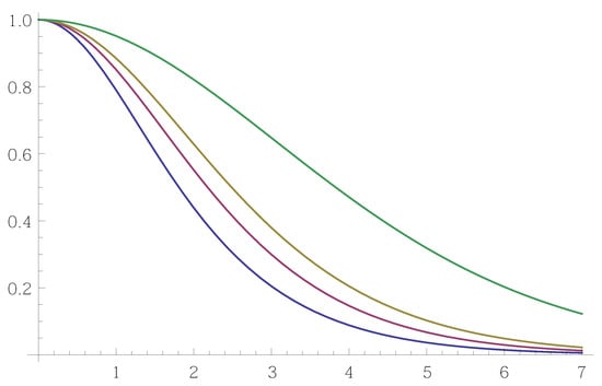
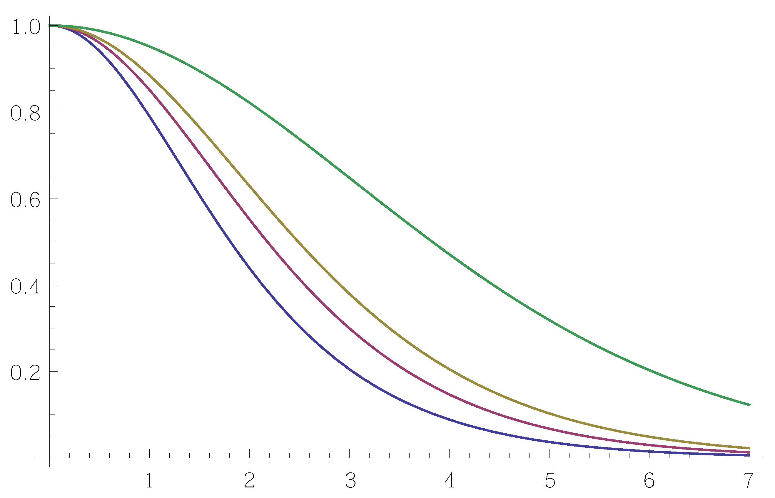
The Radon–Nikodym derivative, or the “killing constant”, ${\psi }_n\left(\mu \right)$, is rather complicated. However, some of its properties are easy to see (cf. Figure 1):

Figure 1. Function ${\psi }_n$ with (from bottom to top) $n=2,3,4,10$.

(i)

${\psi }_n\left(\mu \right)$ is continuous in μ,

(ii)

${\psi }_n\left(\mu \right)$ is strictly decreasing in μ,

(iii)

${\psi }_n\left(\mu \right)\to 0$ as $\mu \to \infty$,

(iv)

${\psi }_n\left(\mu \right)\to 1$ as $\mu \to 0$,

(v)

${\psi }_n\left(\mu \right)$ is increasing in n.

The items (i)–(iv) are clear, because ${\psi }_n\left(\mu \right)$ is the probability that an exponentially killed Brownian motion starting from the origin and with killing intensity ${\mu }^2/2$ is not killed before it hits the boundary of the unit ball. A non-probabilistic argument for (i)–(iv) is to note that

$${\psi }_n\left(\mu r\right)={\mathbb{E}}^0\left[e^{-\frac{{\mu }^2}{2}{\tau }_r^n}\right]$$

and to use the monotone convergence. The item (v) is somewhat surprising: the higher the dimension n, the more likely it is for the killed Brownian motion to survive to the boundary of the unit ball. A possible intuitive explanation is that the higher the dimension, the more transitive the unit ball is, combined with the remarkable result by Ciesielski and Taylor [21] that the probability distribution for the total time spent in a ball by $(n+2)$-dimensional Brownian motion is the same as the probability distribution of the hitting time of n-dimensional Brownian motion on the boundary of the ball.

Corollary 5.

Let $\mu >0$, and let u be μ-panharmonic on the entire space ${\mathbb{R}}^n$. If u is bounded, then $u\equiv 0$.

Proof. 

By Theorem 4,

$$\begin{array}{c}{\displaystyle \left|u\left(x\right)-u\left(0\right)\right|}\hfill \\ =\left|{\psi }_n\left(\mu r\right){\int }_{\partial B_n(x,r)}u\left(y\right){\sigma }_n(r;\mathrm{d}y)-{\psi }_n\left(\mu r\right){\int }_{\partial B_n(0,r)}u\left(y\right){\sigma }_n(r;\mathrm{d}y)\right|\hfill \\ \le \left|{\psi }_n\left(\mu r\right){\int }_{\partial B_n(x,r)}u\left(y\right){\sigma }_n(r;\mathrm{d}y)\right|+\left|{\psi }_n\left(\mu r\right){\int }_{\partial B_n(0,r)}u\left(y\right){\sigma }_n(r;\mathrm{d}y)\right|\hfill \\ \le 2{\psi }_n\left(\mu r\right){\parallel u\parallel }_{\infty },\hfill \end{array}$$

which tends to 0 as $r\to \infty$ by property (iii) of Remark 5. This shows that u is constant. However, for a constant u, the Yukawa equation (Equation (1)) yields $0={\mu }^{2}u$, which implies that $u\equiv 0$. ☐

5. Discussion on Extensions and Simulation

The Yukawa equation (Equation (1)) is a special case of the Schrödinger equation:

$$\Delta u\left(x\right)=q\left(x\right)u\left(x\right).$$

(16)

The Schrödinger equation and its connection to the Brownian motion has been studied, for example, by Chung and Zhao [8]. Our investigation here can be seen as a special case. For example, analogs of Theorem 1 and Corollary 1 are known for the Schrödinger equation. However, analogs of the Duffin correspondence (Equation (11)) and Corollary 2 are not known even to exist. Moreover, the results given here cannot easily be calculated for the Schrödinger equation. The problem is that the prospective Radon–Nikodym derivate of the measure associated with the solutions of the Schrödinger equation with respect to the harmonic measure takes the form

$$Z_q^x(D;y)={\mathbb{E}}^x\left[e_q\left({\tau }_D\right)|W\left({\tau }_D\right)=y\right],$$

(17)

where

$$e_q\left(t\right)=e^{-\frac{1}{2}{\int }_0^{t}q\left(W\left(s\right)\right)\mathrm{d}s}$$

is the Feynman–Kac functional. Thus, we see that in order to calculate the Radon–Nikodym derivative, we need to know the joint density of the Feynman–Kac functional and the Brownian motion when the Brownian motion hits the boundary $\partial D$. If q is constant, that is, we have either the Yukawa equation or the Helmholtz equation, then it is enough to know the joint distribution of the hitting time and place of the Brownian motion on the boundary $\partial D$. These distributions are well studied (see, e.g., [14,16,21,22,23]), but few joint distributions involving the Feynman–Kac functionals are known.

In addition to the Yukawa equation, the other important special case of the Schrödinger equation (Equation (16)) is the Helmholtz equation:

$$\Delta u\left(x\right)=-\lambda u\left(x\right),\lambda \ge 0.$$

(18)

It is possible to also provide a Duffin correspondence for the Helmholtz equation. Indeed, for example, setting

$$\overline{u}\left(\overline{x}\right)=\overline{u}(x,\tilde{x})=u\left(x\right)cosh\left(\lambda \tilde{x}\right)$$

provides a correspondence (see [24] for details). Thus, our results extend in a straightforward manner to the Helmholtz equation (Equation (18)) for domains that are small enough with respect to the creation parameter $\lambda$ that the associated Feynman–Kac functional is finite:

$${\mathbb{E}}^x\left[e^{\frac{\lambda }{2}{\tau }_D}\right]<\infty .$$

(19)

Finally, we note that Theorem 1, Corollary 1 and Corollary 2 give three different ways to simulate the panharmonic measures. Indeed, in [24,25], the classical WOS algorithm given by Muller [26] was extended for the Yukawa PDE, and also for the Helmholtz PDE, by using the results mentioned above.

References

- Bishop, C.J.; Jones, P.W. Harmonic measure and arclength. Ann. Math. 1990, 132, 511–547. [Google Scholar] [CrossRef]
- Gehring, F.W.; Hag, K. The Ubiquitous Quasidisk; No. 184.; American Mathematical Society: Providence, RI, USA, 2012. [Google Scholar]
- Krzyż, J.G. Quasicircles and harmonic measure. Ann. Acad. Sci. Fenn. 1987, 12, 19–24. [Google Scholar] [CrossRef]
- Garnett, J.B.; Marshall, D.E. Harmonic Measure; Cambridge University Press: Cambridge, UK, 2005. [Google Scholar]
- Harrach, B. On uniqueness in diffuse optical tomography. Inverse Probl. 2009, 25, 1–14. [Google Scholar] [CrossRef]
- Duffin, R.J. Yukawan potential theory. J. Math. Anal. Appl. 1971, 35, 105–130. [Google Scholar] [CrossRef]
- Duffin, R.J. Hilbert transforms in Yukawan potential theory. Proc. Nat. Acad. Sci. USA 1972, 69, 3677–3679. [Google Scholar] [CrossRef] [PubMed]
- Chung, K.L.; Zhao, Z. From Brownian Motion to Schrödinger’s Equation, 2nd ed.; Springer: Berlin/Heidelberg, Germany, 2001. [Google Scholar]
- Doob, J.L. Classical Potential Theory and Its Probabilistic Counterpart; Grundlehren der Mathematischen Wissenschaften 262; Springer: New York, NY, USA, 1984. [Google Scholar]
- Port, S.C.; Stone, C.J. Brownian Motion and Classical Potential Theory; Academic Press: New York, NY, USA, 1978. [Google Scholar]
- Evans, L.C. Partial Differential Equations (Graduate Studies in Mathematics), 2nd ed.; American Mathematical Society: Providence, RI, USA, 2010. [Google Scholar]
- Kakutani, S. On Brownian motion in n-space. Proc. Imp. Acad. 1944, 20, 648–652. [Google Scholar] [CrossRef]
- Kallenberg, O. Foundations of Modern Probability, 2nd ed.; Springer: New York, NY, USA, 2002. [Google Scholar]
- Borodin, A.; Salminen, P. Handbook of Brownian Motion—Facts and Formulae, 2nd ed.; Birkhäuser: Basel, Switzerland, 2002. [Google Scholar]
- Durrett, R. Stochastic Calculus: A Practical Introduction; CRC Press: Boca Raton, FL, USA, 1996. [Google Scholar]
- Hsu, P. Brownian exit distribution of a ball. In Seminar on Stochastic Processes 1985; Birkhäuser: Boston, MA, USA, 1986. [Google Scholar]
- Dahlberg, B. Estimates of harmonic measure. Arch. Rat. Mech. Anal. 1977, 65, 275–288. [Google Scholar] [CrossRef]
- Makarov, N.G. On the Distortion of Boundary Sets Under Conformal Maps. Proc. Lond. Math. Soc. 1985, 52, 369–384. [Google Scholar] [CrossRef]
- Riesz, F.; Riesz, M. Über die Randwerte einer analytischen Funktion. In Quatrième Congrès des Mathématiciens Scandinaves; Stockholm, Sweden, 1916; pp. 27–44. [Google Scholar]
- Wendel, J.G. Hitting Spheres with Brownian Motion. Ann. Probab. 1980, 8, 164–169. [Google Scholar] [CrossRef]
- Ciesielski, Z.; Taylor, S.J. First passage times and sojourn times for Brownian motion in space and the exact Hausdorff measure of the sample path. Trans. Am. Math. Soc. 1962, 103, 434–450. [Google Scholar] [CrossRef]
- Kent, T. Eigenvalue expansion for diffusion hitting times. Z. Wahrscheinlichkeitstheorie Ver. Gebiete 1980, 52, 309–319. [Google Scholar] [CrossRef]
- Lévy, P. La mesure de Hausdorff de la courbe du mouvement brownien. Giorn. Ist. Ital. Attuari 1953, 16, 1–37. [Google Scholar]
- Yang, X.; Rasila, A.; Sottinen, T. Walk On Spheres Algorithm for Helmholtz and Yukawa Equations via Duffin Correspondence. Methodol. Comput. Appl. Probab. 2017, 19, 589–602. [Google Scholar] [CrossRef]
- Yang, X.; Rasila, A.; Sottinen, T. Efficient simulation of Schrödinger equation with piecewise constant positive potential. arXiv, 2015; arXiv:1512.01306. [Google Scholar]
- Muller, M.E. Some continuous Monte Carlo methods for the Dirichlet problem. Ann. Math. Stat. 1956, 27, 569–589. [Google Scholar] [CrossRef]
© 2018 by the authors. Licensee MDPI, Basel, Switzerland. This article is an open access article distributed under the terms and conditions of the Creative Commons Attribution (CC BY) license (http://creativecommons.org/licenses/by/4.0/).