The Second Immanantal Polynomial for the Signless Laplacian Matrix of a Graph

Abstract

The second immanantal polynomial is one of the important directions in algebraic theory. Let $M=\left[m_{ij}\right]$ be an $n\times n$ matrix. The second immanant of matrix M is defined as $d_2\left(M\right)={\sum }_{\sigma \in S_n}\chi \left(\sigma \right){\prod }_{i=1}^n{m}_{i\sigma \left(i\right)}$, where $\chi$ is the irreducible character of the symmetric group $S_n$ of degree n, corresponding to the partition $(2^1,1^{n-2})$. Let G be a graph with n vertices. Denote by $Q\left(G\right)$ the signless Laplacian matrix of G. The second signless Laplacian immanantal polynomial of G is defined as $d_2(xI-Q\left(G\right))={\sum }_{k=0}^n{(-1)}^k{c}_k\left(G\right)x^{n-k}$, where $c_k\left(G\right)$ is the coefficient of this polynomial. This paper investigates fundamental properties of this polynomial. First, we give combinatorial expressions for the first few coefficients of the second signless Laplacian immanantal polynomial. Next, we prove that the polynomial has no zero or negative real roots for connected graphs. Furthermore, we show that there is an equivalence relation among three polynomials for regular graphs, which implies that if two regular graphs share the same characteristic polynomial, then they also share the same second signless Laplacian immanantal polynomial. Finally, we prove that paths and almost complete graphs are determined by their second signless Laplacian immanantal polynomials.

1. Introduction

Let $S_n$ be the permutation group on n symbols and $\lambda$ be a partition of n, and let ${\chi }_{\lambda }$ be the irreducible character of $S_n$ corresponding to the partition $\lambda$. The immanant function $d_{\lambda }$ associated with the character ${\chi }_{\lambda }$ acting on an $n\times n$ matrix $M=\left[m_{ij}\right]$ is defined as

$$\begin{array}{c}\hfill d_{\lambda }\left(M\right)=\sum _{\sigma \in S_n}{\chi }_{\lambda }\left(\sigma \right)\prod _{i=1}^n{m}_{i\sigma \left(i\right)}.\end{array}$$

In particular, when $\lambda =(k,1^{n-k})$, we call $d_{(k,1^{n-k})}\left(M\right)$ the hook immanant of M, abbreviated as $d_k\left(M\right)$. The determinant $\det \left(M\right)$, second immanant $d_2\left(M\right)$ and permanent $per\left(M\right)$ are the immanants corresponding to $\lambda =\left(1^n\right)$, $\lambda =(2^1,1^{n-2})$ and $\lambda =\left(n\right)$, respectively.

Let $G=\left(V\right(G),E(G\left)\right)$ be a simple graph with vertex set $V\left(G\right)=\{v_1,v_2,\dots ,v_n\}$ and edge set $E\left(G\right)=\{e_1,e_2,\dots ,e_m\}$, and let $d_i$ be the degree of vertex $v_i$. Denote by $D\left(G\right)$ the diagonal matrix with diagonal elements $d_1,d_2,\dots ,d_n$. For graph G, its adjacency matrix is $A\left(G\right)=\left(a_{ij}\right)$, where $a_{ij}=1$ if $v_i$ and $v_j$ are adjacent and $a_{ij}=0$ otherwise. The Laplacian matrix $L\left(G\right)$ and the signless Laplacian matrix $Q\left(G\right)$ of graph G are respectively defined as follows:

$$\begin{array}{ccc}\hfill L\left(G\right)& =& D\left(G\right)-A\left(G\right),\hfill \\ \hfill Q\left(G\right)& =& D\left(G\right)+A\left(G\right).\hfill \end{array}$$

The determinant and permanent of matrices $L\left(G\right)$ and $Q\left(G\right)$ have been extensively studied [1,2,3,4,5]. But the properties of the analogous second immanant remain less explored. This gap is the focus of our work.

The immanantal polynomial of an $n\times n$ matrix is $d_{\lambda }(xI-M)$, and $c_{\lambda ,k}\left(M\right)$ is the coefficient of this polynomial, defined as follows:

$$d_{\lambda }(xI-M)=\sum _{k=0}^n{(-1)}^k{c}_{\lambda ,k}\left(M\right)x^{n-k}.$$

The characteristic polynomial, second immanantal polynomial and permanent polynomial of a matrix M are denoted by $\det (M,x)$, $d_2(M,x)$ and $\mathrm{per}(M,x)$, respectively, defined as follows:

$$\begin{array}{c}\hfill \det (M,x)=\det (xI-M),d_2(M,x)=d_2(xI-M),\mathrm{per}(M,x)=\mathrm{per}(xI-M),\end{array}$$

where I is an $n\times n$ identity matrix.

Let $R=\left[r_{st}\right]$ be a $l\times l$ matrix $(l\ge 2)$, and let $R\left(s\right)$ be the submatrix of R formed by deleting the s-th row and column of R. The determinant and second immanant of R are respectively denoted as $\det \left(R\right)$ and $d_2\left(R\right)$. Merris [6] gave a result that the second immanant of matrix R satisfies:

$$d_2\left(R\right)=\sum _{s=1}^l{r}_{ss}\det \left(R\left(s\right)\right)-\det \left(R\right).$$

(1)

Currently, numerous results exist on determinants [1,7,8,9]. Some scholars have also investigated problems related to permanents [10,11,12,13]. Merris [6] first introduced the second immanantal polynomial for the Laplacian matrix of graphs and examined its coefficients and properties. Subsequent work by Wu et al. [14,15] further explored properties of this polynomial. Bürgisser [16] showed that computing the immanant is VNP-complete, so that the computation of immanantal polynomials is very difficult. There have been some studies on the immanantal polynomials of the Laplacian matrix [17,18,19,20,21]. Yu et al. [22] established that the immanantal polynomials of the Laplacian and signless Laplacian matrices are the same for bipartite graphs. But the study of immanantal polynomials in non-bipartite graphs is still unclear. Therefore, the study of immanantal polynomials of the signless Laplacian matrix for non-bipartite graphs is our main goal. In this paper, we study the fundamental algebraic and spectral properties of the second immanantal polynomial of the signless Laplacian matrix for non-bipartite graphs and obtain the expressions for the first few coefficients of this polynomial and some properties of its roots.

The remainder of this paper is structured in the following manner. In Section 2, we investigate coefficients of the second signless Laplacian immanantal polynomial of graphs. Explicit expressions for several coefficients are derived, and related inequalities are established. In Section 3, we study properties of the roots of this polynomial and provide conditions under which a graph is determined by its polynomial. Additionally, we conclude that paths and almost-complete graphs are determined by their second signless Laplacian immanantal polynomials based solely on the first few coefficients identified in Section 2. Finally, a summary of the work is presented.

2. Coefficients of the Second Signless Laplacian Immanantal Polynomial

In this section, we primarily investigate the coefficients of the second signless Laplacian immanantal polynomial of a graph. The second signless Laplacian immanantal polynomial of the graph G is defined as:

$$\begin{array}{c}\hfill d_2(xI-Q\left(G\right))=c_0\left(G\right)x^n-c_1\left(G\right)x^{n-1}+\cdots +{(-1)}^n{c}_n\left(G\right).\end{array}$$

Merris [6] studied the second immanantal polynomial of an $n\times n$ matrix $M=\left[m_{ij}\right]$ and established relations for its coefficients. The set of subsets of $\{1,2,\dots ,n\}$ with k elements is denoted by $Q_{k,n}$. For $B\in Q_{k,n}$, let $M\left[B\right]$ be the $k\times k$ principal submatrix of M corresponding to B. Merris [6] proposed that the coefficient $c_k\left(M\right)$ of ${(-1)}^k{x}^{n-k}$ in the expansion of the second immanantal polynomial $d_2(xI-M)$ of matrix M satisfies:

$$c_k\left(M\right)=(\sum _{B\in Q_{k-1,n}}(\sum _{t\notin B}{m}_{tt})\det M\left[B\right])+(n-k-1)q_k\left(M\right),$$

(2)

where $q_k\left(M\right)$ is the coefficient of ${(-1)}^k{x}^{n-k}$ in the expansion of the characteristic polynomial $\det (xI-M)$. Furthermore, several coefficients of the second Laplacian immanantal polynomial of the graph are provided.

Lemma 1

(Merris, [6]). Let G be a graph with n vertices and m edges, and define $L\left(G\right)$ as the Laplacian matrix of G, and

$$\begin{array}{c}\hfill d_2(xI-L\left(G\right))=\sum _{k=0}^n{(-1)}^k{f}_k\left(G\right)x^{n-k},\end{array}$$

then

$$\begin{array}{c}\hfill f_n\left(G\right)=2m\tau \left(G\right),\end{array}$$

where $\tau \left(G\right)$ is the number of spanning trees in graph G.

Lemma 2

(Biggs, [7]). Let $\det (A\left(G\right),x)={\sum }_{k=0}^n{(-1)}^k{q}_k\left(G\right)x^{n-k}$; then

$$\begin{array}{ccc}& & q_0\left(G\right)=1,q_1\left(G\right)=0,q_2\left(G\right)=-m,q_3\left(G\right)=2T\left(G\right),\hfill \\ & & q_4\left(G\right)=\left({\displaystyle \genfrac{}{}{0pt}{}{m}{2}}\right)-\sum _{i=1}^n\left({\displaystyle \genfrac{}{}{0pt}{}{d_i}{2}}\right)-2C_4,\hfill \end{array}$$

where $T\left(G\right)$ is the number of triangles in graph G, and $C_4$ is the number of quadrangles in graph G.

We primarily study the signless Laplacian matrix $Q\left(G\right)$ of a graph. By Equation (2), let $M=Q\left(G\right)$; we obtain:

$$c_k\left(Q\left(G\right)\right)=\sum _{B\in Q_{k-1,n}}(\sum _{t\notin B}{d}_t)\det Q\left(G\right)\left[B\right]+(n-k-1)q_k\left(Q\left(G\right)\right),$$

(3)

when G is a regular graph and its regularity is r, then:

$$c_k\left(Q\left(G\right)\right)=(n-k+1)r{q}_{k-1}\left(Q\left(G\right)\right)+(n-k-1)q_k\left(Q\left(G\right)\right).$$

(4)

Let $e=\{s,t\}\in E\left(G\right)$, and let $(d_1,d_2,\dots ,d_n)$ be the degree sequence of graph G. Denote $D_e\left(G\right)$ by the diagonal matrix obtained from $D\left(G\right)$ by deleting $d_s$ and $d_t$. Define $a_l$ as the l-th elementary symmetric function, with $a_l\left(G\right)=a_l\left(D\left(G\right)\right)={\sum }_{1\le <i_1<\dots <i_l\le n}{d}_{i_1}\cdots d_{i_l}$. When $l⩾3$, let

$$\begin{array}{c}\hfill b_l\left(G\right)=\sum _{e\in E\left(G\right)}{a}_{l-2}\left(D_e\left(G\right)\right).\end{array}$$

Lemma 3

(Yu and Qu, [22]). Let G be a graph with n vertices, and let $Q\left(G\right)$ be its signless Laplacian matrix. The immanantal polynomial of the signless Laplacian matrix of G is as follows:

$$d_{\lambda }(xI-Q\left(G\right))=\sum _{k=0}^n{(-1)}^k{c}_{\lambda ,k}\left(Q\left(G\right)\right)x^{n-k},$$

then

$$c_{\lambda ,k}\left(Q\left(G\right)\right)=\sum _{B:\left|B\right|=k,B\subseteq V\left(G\right)}\sum _C{\chi }_{\lambda }\left(C\right)\sum _{\sigma \in C}\prod _{i\in B;i=\sigma \left(i\right)}{d}_i,$$

(5)

where B is a k-subset of $V\left(G\right)$, C is a conjugacy class of the subgroup ${\left(S_n\right)}_B$, and $d_i$ is the degree of vertex $v_i$.

The second immanant of matrix M is expressed as follows:

$$d_2\left(M\right)=\sum _{\sigma \in S_n}{\chi }_2\left(\sigma \right)\prod _{i=1}^n{m}_{i\sigma \left(i\right)},$$

(6)

where ${\chi }_2$ stands for the irreducible character of $S_n$ associated to the partition $(2^1,1^{n-2})$. In particular, ${\chi }_2\left(\sigma \right)=\epsilon \left(\sigma \right)[F\left(\sigma \right)-1]$, where $\epsilon$ is the alternating character and F is the number of fixed points.

Let G be a graph with vertex set $V\left(G\right)=\{v_1,v_2,\dots ,v_n\}$, and let $d_i$ be the degree of vertex $v_i$. $K\subseteq \{1,2,\dots ,n\}$, and let H be a subgraph of G with vertices $v_i$ where $i\in K$, such that all connected components of H can only be an edge or a cycle. Define $\left|K\right|$ as the number of vertices in graph H. Denote by $\mathcal{H}$ the set of all subgraphs H. By Equations (5) and (6), when $\lambda =2,k=n$, we have ${\chi }_2\left(\sigma \right)=\epsilon \left(\sigma \right)[F\left(\sigma \right)-1]={(-1)}^{\left|K\right|-c^{\prime }\left(H\right)}(n-|K|-1)$, where $c^{\prime }\left(H\right)$ is the number of components in H. If H contains cycle components, they have clockwise and counterclockwise directions. Therefore, we obtain the following corollary.

Corollary 1.

Let G be a graph with n vertices, and let $Q\left(G\right)$ be its signless Laplacian matrix. Denote by $c_k\left(G\right)$ the coefficient of ${(-1)}^k{x}^{n-k}$ in the polynomial $d_2(xI-Q\left(G\right))$. Then

$$\begin{array}{c}\hfill c_n\left(G\right)=\sum _{K\subseteq \{1,2,\dots ,n\}}\sum _{H\in \mathcal{H}}{(-1)}^{\left|K\right|-c^{\prime }\left(H\right)}(n-|K|-1)2^{c\left(H\right)}\prod _{i\notin K}{d}_i,\end{array}$$

where $c^{\prime }\left(H\right)$ is the number of components in H, and $c\left(H\right)$ is the number of cycle components of H.

Theorem 1.

Let G be a graph with n vertices and m edges, and let E be the edge set of G. Denote by $Q\left(G\right)$ the signless Laplacian matrix of G, and

$$\begin{array}{c}\hfill d_2(xI-Q\left(G\right))=\sum _{k=0}^n{(-1)}^k{c}_k\left(G\right)x^{n-k},\end{array}$$

then

$$\begin{array}{ccc}\hfill c_0\left(G\right)& =& n-1,\hfill \\ \hfill c_1\left(G\right)& =& (n-1)a_1\left(G\right)=2m(n-1),\hfill \\ \hfill c_2\left(G\right)& =& (n-1)a_2\left(G\right)-m(n-3)(n⩾3)a_2\left(G\right)=a_2\left(D\left(G\right)\right)=\sum _{1\le i<j\le n}{d}_i{d}_j,\hfill \\ \hfill c_3\left(G\right)& =& (n-1)a_3\left(G\right)-(n-3)b_3\left(G\right)+2(n-4)T\left(G\right)(n⩾4)b_3\left(G\right)=\sum _{e\in E}{a}_1\left(D_e\left(G\right)\right),\hfill \\ \hfill c_4\left(G\right)& =& (n-1)a_4\left(G\right)-(n-3)b_4\left(G\right)+(n-5)[\left({\displaystyle \genfrac{}{}{0pt}{}{m}{2}}\right)-\sum _{i=1}^n\left({\displaystyle \genfrac{}{}{0pt}{}{d_i}{2}}\right)-2C_4]\hfill \\ & & +2(n-4)\sum _{i=1}^n{d}_i[T\left(G\right)-T\left(G\left(v_i\right)\right)],\hfill \end{array}$$

where $T\left(G\right)$ is the number of triangles in graph G, $T\left(G\right(v\left)\right)$ is the number of triangles containing vertex v in graph G and $C_4$ is the number of quadrangles (cycles of length 4) in graph G.

Proof. 

By Equation (6), let $M=xI-Q\left(G\right)$, then $c_0\left(G\right)={\chi }_2\left(\mathrm{id}\right)=n-1$. The coefficient $c_1\left(G\right)$ is equal to the product of the trace of $Q\left(G\right)$ and ${\chi }_2\left(\mathrm{id}\right)$, so $c_1\left(G\right)=(n-1)a_1\left(G\right)=2m(n-1)$. When $n⩾3$, the coefficient of $x^{n-2}$ has two sources: One is when $\sigma =\mathrm{id}$, which contributes $(n-1)a_2\left(G\right)$; the other is when it constitutes a set of vertex exchanges forming an edge, so then ${\chi }_2=-(n-3)$ and there are m edges, contributing $-m(n-3)$. Therefore, $c_2\left(G\right)=(n-1)a_2\left(G\right)-m(n-3)$.

When $n⩾4$, the coefficient of $x^{n-3}$ has three sources: one is when $\sigma =\mathrm{id}$, which contributes $(n-1)a_3\left(G\right)$; next is the set of vertex exchanges that form an edge, which contributes $-(n-3)b_3\left(G\right)$; the third is 3-cycle $\sigma =\left(stl\right)$, where $\{s,t\},\{t,l\},\{s,l\}$ are edges. For a 3-cycle $\sigma$, the irreducible character ${\chi }_2\left(\sigma \right)=\epsilon \left(\sigma \right)[F\left(\sigma \right)-1]=1·[(n-3)-1]=n-4$. Moreover, each triangle in graph G has both clockwise and counterclockwise orientations. Lastly, as the entries $\{s,t\},\{t,l\},\{s,l\}$ of $Q\left(G\right)$ corresponding to the edges of a triangle are all 1, the total contribution from 3-cycles is $2(n-4)T\left(G\right)$. Therefore, $c_3\left(G\right)=(n-1)a_3\left(G\right)-(n-3)b_3\left(G\right)+2(n-4)T\left(G\right)$.

First, we introduce some notation. Let $T\left(G\right(v\left)\right)$ denote the number of triangles in graph G that contain vertex v. Let $v_{r_1},v_{r_2},\cdots ,v_{r_i}$ be i distinct vertices in G, and let $G_{r_1,r_2,\cdots ,r_i}$ be the subgraph obtained by deleting vertices $v_{r_1},v_{r_2},\cdots ,v_{r_i}$ from G. We use $G\left[l_r\right]$ to represent the graph obtained by attaching a loop of weight $l_r$ at vertex $v_r$. Similarly, denote by $G[l_r,l_s]$ the graph obtained by attaching loops with weights $l_r$ and $l_s$ at vertices $v_r$ and $v_s$, respectively. Finally, $G[l_1,l_2,\dots ,l_n]$ is the graph obtained by attaching a loop of weight $l_r$ at each vertex $v_r(r=1,2,\dots ,n)$. Define the adjacency matrix $A\left(G[l_{r_1},l_{r_2},\dots ,l_{r_s}]\right)$ of $G[l_{r_1},l_{r_2},\dots ,l_{r_s}]$ as the $n\times n$ matrix $\left(a_{ij}\right)$, where

$$\begin{array}{c}\hfill a_{ij}=\left\{\begin{array}{cc}{l}_r,\hfill & \mathrm{if}i=j=r,r\in \{r_1,r_2,\dots ,r_s\},\hfill \\ 1,\hfill & \mathrm{if}i\ne j\mathrm{and}{v}_i{v}_j\in E\left(G\right),\hfill \\ 0,\hfill & \mathrm{otherwise}.\hfill \end{array}\right.\end{array}$$

By expanding the determinant, we obtain

$$\det (A\left(G\left[l_r\right]\right),x)=\det (A\left(G\right),x)-l_r\det (A\left(G_r\right),x).$$

(7)

By Equations (1) and (7), we have

$$\begin{array}{ccc}\hfill & & d_2(A\left(G\left[l_r\right]\right),x)\hfill \\ & =& \sum _{\begin{array}{c}i=1\\ i\ne r\end{array}}^{n}x\det (A\left(G_i\left[l_r\right]\right),x)+(x-l_r)\det (A\left(G_r\right),x)-\det (A\left(G\right),x)+l_r\det (A\left(G_r\right),x)\hfill \\ & =& \sum _{\begin{array}{c}i=1\\ i\ne r\end{array}}^{n}x(\det (A\left(G_i\right),x)-l_r\det (A\left(G_{i,r}\right),x))+x\det (A\left(G_r\right),x)-\det (A\left(G\right),x)\hfill \\ & =& \sum _{i=1}^{n}x\det (A\left(G_i\right),x)-\det (A\left(G\right),x)-\sum _{\begin{array}{c}i=1\\ i\ne r\end{array}}^{n}x·l_r\det (A\left(G_{i,r}\right),x)\hfill \\ & =& d_2(A\left(G\right),x)-\sum _{\begin{array}{c}i=1\\ i\ne r\end{array}}^{n}x·l_r\det (A\left(G_{i,r}\right),x)\hfill \\ & =& d_2(A\left(G\right),x)-l_r{d}_2(A\left(G_r\right),x)-l_r\det (A\left(G_r\right),x).\hfill \end{array}$$

(8)

With $G[l_r,l_s]$ repeated application on Equation (8), we obtain

$$\begin{array}{ccc}& & d_2(A\left(G[l_r,l_s]\right),x)\hfill \\ & =& d_2(A\left(G\left[l_r\right]\right),x)-l_s{d}_2(A\left(G_s\left[l_r\right]\right),x)-l_s\det (A\left(G_s\left[l_r\right]\right),x)\hfill \\ & =& d_2(A\left(G\right),x)-l_r{d}_2(A\left(G_r\right),x)-l_r\det (A\left(G_r\right),x)-l_s{d}_2(A\left(G_s\right),x)+l_s{h}_r{d}_2(A\left(G_{s,r}\right),x)\hfill \\ & & +l_s{l}_r\det (A\left(G_{s,r}\right),x)-l_s\det (A\left(G_s\right),x)+l_s{l}_r\det (A\left(G_{s,r}\right),x)\hfill \\ & =& d_2(A\left(G\right),x)-l_r{d}_2(A\left(G_r\right),x)-l_s{d}_2(A\left(G_s\right),x)+l_s{h}_r{d}_2(A\left(G_{s,r}\right),x)-l_r\det (A\left(G_r\right),x)\hfill \\ & & -l_s\det (A\left(G_s\right),x)+2l_s{l}_r\det (A\left(G_{s,r}\right),x).\hfill \end{array}$$

With respect to the loops on all n vertices, we conduct additional iterations, and thus we obtain the expression

$$\begin{array}{ccc}\hfill & & d_2(A\left(G[l_1,l_2,\dots ,l_n]\right),x)\hfill \\ & =& d_2(A\left(G\right),x)+\sum _{i=1}^n{(-1)}^i\sum _{1\le r_1<\cdots <r_i\le n}{l}_{r_1}\cdots l_{r_i}{d}_2(A\left(G_{r_1,\dots ,r_i}\right),x)\hfill \\ & & +\sum _{i=1}^n{(-1)}^i·i·\sum _{1\le r_1<\cdots <r_i\le n}{l}_{r_1}\cdots l_{r_i}\det (A\left(G_{r_1,\dots ,r_i}\right),x).\hfill \end{array}$$

(9)

Consider a graph G with degree sequence $(d_1,d_2,\dots ,d_n)$. It then follows that the signless Laplacian matrix $Q\left(G\right)$ is the exact adjacency matrix of $G[d_1,d_2,\dots ,d_n]$. Therefore, by Equation (9) we obtain the following expression.

$$\begin{array}{ccc}\hfill d_2(Q\left(G\right),x)& =& d_2(A\left(G\right),x)+\sum _{i=1}^n{(-1)}^i\sum _{1\le r_1<\cdots <r_i\le n}{d}_{r_1}\cdots d_{r_i}{d}_2(A\left(G_{r_1,\dots ,r_i}\right),x)\hfill \\ & & +\sum _{i=1}^n{(-1)}^i·i·\sum _{1\le r_1<\cdots <r_i\le n}{d}_{r_1}\cdots d_{r_i}\det (A\left(G_{r_1,\dots ,r_i}\right),x).\hfill \end{array}$$

(10)

Let

$$\begin{array}{ccc}\hfill \det \left(A\right(G),x)& =& \sum _{k=0}^n{(-1)}^k{q}_k\left(G\right)x^{n-k},\hfill \\ \hfill d_2(A\left(G\right),x)& =& \sum _{k=0}^n{(-1)}^k{p}_k\left(G\right)x^{n-k},\hfill \\ \hfill d_2(Q\left(G\right),x)& =& \sum _{k=0}^n{(-1)}^k{c}_k\left(G\right)x^{n-k},\hfill \end{array}$$

where $1\le k\le n$. By Equation (2), we have $p_k\left(G\right)=(n-k-1)q_k\left(G\right)$. By Equation (10) we obtain

$$\begin{array}{ccc}& & {(-1)}^k{c}_k\left(G\right)\hfill \\ & =& {(-1)}^k{p}_k\left(G\right)+\sum _{i=1}^n{(-1)}^i\sum _{1\le r_1<\cdots <r_i\le n}{d}_{r_1}\cdots d_{r_i}{(-1)}^{k-i}{p}_{k-i}\left(G_{r_1,\dots ,r_i}\right)\hfill \\ & & +\sum _{i=1}^n{(-1)}^i·i·\sum _{1\le r_1<\cdots <r_i\le n}{d}_{r_1}\cdots d_{r_i}{(-1)}^{k-i}{q}_{k-i}\left(G_{r_1,\dots ,r_i}\right)\hfill \\ & =& {(-1)}^k(n-k-1)q_k\left(G\right)+\sum _{i=1}^n{(-1)}^k\sum _{1\le r_1<\cdots <r_i\le n}{d}_{r_1}\cdots d_{r_i}(n-k-1)q_{k-i}\left(G_{r_1,\dots ,r_i}\right)\hfill \\ & & +\sum _{i=1}^n{(-1)}^k·i·\sum _{1\le r_1<\cdots <r_i\le n}{d}_{r_1}\cdots d_{r_i}{q}_{k-i}\left(G_{r_1,\dots ,r_i}\right),\hfill \end{array}$$

then

$$\begin{array}{ccc}\hfill c_k\left(G\right)& =& (n-k-1)q_k\left(G\right)+\sum _{i=1}^n\sum _{1\le r_1<\cdots <r_i\le n}{d}_{r_1}\cdots d_{r_i}(n-k+i-1)q_{k-i}\left(G_{r_1,\dots ,r_i}\right).\hfill \end{array}$$

By Lemma 2, it can be deduced that

$$\begin{array}{ccc}\hfill c_4\left(G\right)& =& (n-5)q_4\left(G\right)+\sum _{i=1}^n{d}_i(n-4)q_3\left(G_i\right)+\sum _{1\le i<j\le n}{d}_i{d}_j(n-3)q_2\left(G_{i,j}\right)\hfill \\ & & +\sum _{1\le i<j<k\le n}{d}_i{d}_j{d}_k(n-2)q_1\left(G_{i,j,k}\right)+\sum _{1\le i<j<k<l\le n}{d}_i{d}_j{d}_k{d}_l(n-1)q_0\left(G_{i,j,k,l}\right)\hfill \\ & =& (n-5)[\left({\displaystyle \genfrac{}{}{0pt}{}{m}{2}}\right)-\sum _{i=1}^n\left({\displaystyle \genfrac{}{}{0pt}{}{d_i}{2}}\right)-2C_4]+2(n-4)\sum _{i=1}^n{d}_i[T\left(G\right)-T\left(G\left(v_i\right)\right)]\hfill \\ & & -(n-3)\sum _{1\le i<j\le n}{d}_i{d}_j·\left|E\left(G_{i,j}\right)\right|+(n-1)\sum _{1\le i<j<k<l\le n}{d}_i{d}_j{d}_k{d}_l.\hfill \end{array}$$

According to reference [4], we have

$$\begin{array}{c}\hfill \sum _{1\le i<j\le n}{d}_i{d}_j·\left|E\left(G_{i,j}\right)\right|=\sum _{i=1}^n{d}_i^3-{\displaystyle \frac{5}{2}}m\sum _{i=1}^n{d}_i^2+\sum _{v_i{v}_j\in E\left(G\right)}{d}_i{d}_j+2m^3,\end{array}$$

$$\begin{array}{ccc}\hfill b_4\left(G\right)& =& \sum _{e\in E\left(G\right)}{a}_2\left(D_e\left(G\right)\right)\hfill \\ & =& \sum _{v_i{v}_j\in E\left(G\right)}\sum _{\begin{array}{c}1\le u<v\le n\\ u,v\ne i,j\end{array}}^n{d}_u{d}_v\hfill \\ & =& \sum _{v_i{v}_j\in E\left(G\right)}[\sum _{1\le u<v\le n}{d}_u{d}_v-d_i(2m-d_i)-d_j(2m-d_i-d_j)]\hfill \\ & =& \sum _{v_i{v}_j\in E\left(G\right)}[{\displaystyle \frac{1}{2}}((\sum _{u=1}^n{d}_u{)}^2-\sum _{u=1}^n{d}_u^2)-d_i(2m-d_i)-d_j(2m-d_i-d_j)]\hfill \\ & =& \sum _{v_i{v}_j\in E\left(G\right)}[2m^2-{\displaystyle \frac{1}{2}}\sum _{u=1}^n{d}_u^2-2m{d}_i+d_i^2-2m{d}_j+d_i{d}_j+d_j^2]\hfill \\ & =& 2m^3-{\displaystyle \frac{1}{2}}m\sum _{u=1}^n{d}_u^2-\sum _{v_i{v}_j\in E\left(G\right)}2m(d_i+d_j)+\sum _{v_i{v}_j\in E\left(G\right)}(d_i^2+d_j^2)+\sum _{v_i{v}_j\in E\left(G\right)}{d}_i{d}_j\hfill \\ & =& 2m^3-{\displaystyle \frac{1}{2}}m\sum _{u=1}^n{d}_u^2-2m\sum _{u=1}^n{d}_u^2+\sum _{u=1}^n{d}_u^3+\sum _{v_i{v}_j\in E\left(G\right)}{d}_i{d}_j\hfill \\ & =& \sum _{1\le i<j\le n}{d}_i{d}_j·\left|E\left(G_{i,j}\right)\right|,\hfill \end{array}$$

$$\begin{array}{ccc}\hfill c_4\left(G\right)& =& (n-5)[\left({\displaystyle \genfrac{}{}{0pt}{}{m}{2}}\right)-\sum _{i=1}^n\left({\displaystyle \genfrac{}{}{0pt}{}{d_i}{2}}\right)-2C_4]+2(n-4)\sum _{i=1}^n{d}_i[T\left(G\right)-T\left(G\left(v_i\right)\right)]\hfill \\ & & -(n-3)b_4\left(G\right)+(n-1)a_4\left(G\right).\hfill \end{array}$$

□

We summarize this section using some inequalities of $c_k\left(G\right)$.

Theorem 2.

Let G be a graph with n vertices. Define $a_l\left(G\right)$ as the l-th elementary symmetric function of $D\left(G\right)$, with $c_k\left(G\right)$ defined as the coefficient of ${(-1)}^k{x}^{n-k}$ in the polynomial $d_2(xI-Q\left(G\right))$. Therefore $(n-1)a_k\left(G\right)⩾c_k\left(G\right)⩾0$.

Proof. 

Given that $Q\left(G\right)$ is a positive semidefinite symmetric matrix and every term in Equation (3) is non-negative, for the principal submatrices, we can obtain the following through Hadamard’s determinant inequality.

$$\begin{array}{ccc}\hfill c_k\left(G\right)& ⩽& \sum _{B\in Q_{k-1,n}}(\sum _{t\notin B}d\left(t\right))\prod _{i\in B}d\left(i\right)+(n-k-1)a_k\left(G\right)\hfill \\ & =& k{a}_k\left(G\right)+(n-k-1)a_k\left(G\right)\hfill \\ & =& (n-1)a_k\left(G\right).\hfill \end{array}$$

□

Theorem 3.

Let G be a graph with n vertices, and let H be a spanning subgraph of G. Then $c_k\left(G\right)⩾c_k\left(H\right)$ for $0⩽k⩽n$.

Proof. 

Let $V\left(G\right)$ and $E\left(G\right)$ be the vertex set and edge set of graph G, respectively. G and H have the same vertices, and let $E\left(H\right)$ be the edge set of graph H. Define $\overline{G}$ as a graph with the same set of vertices as G and H, and whose edge set is composed of edges in G that are not in H. Naturally, $Q\left(G\right)=Q\left(H\right)+Q\left(\overline{G}\right)$. If X and Y are two positive semidefinite Hermitian matrices, and they have the same order, then $\det X+\det Y⩽\det (X+Y)$. From Equation (3), it follows that $c_k\left(G\right)⩾c_k\left(H\right)$. □

Lemma 4.

(Yu and Qu, [22]) Assume G is a bipartite graph, then the second immanantal polynomial of the signless Laplacian matrix and the Laplacian matrix of G have the same coefficients.

Lemma 5.

Let G be a graph with n vertices. When $1⩽k⩽n$,

$$\begin{array}{c}\hfill c_k\left(G\right)⩽\left({\displaystyle \genfrac{}{}{0pt}{}{n}{k}}\right){(n-2)}^{k-2}[(n-1)(n-k+2)(n-2)+k^2-k].\end{array}$$

Suppose that G is a connected graph, then $c_k\left(G\right)⩾c_k{\left(T\right)}_{max}$, where T is a spanning tree of G. Then

$$\begin{array}{c}\hfill c_n\left(G\right)⩾2(n-1).\end{array}$$

Proof. 

By Theorem 3, $c_k\left(G\right)⩽c_k\left(K_n\right)$, where $K_n$ is a complete graph, we obtain

$$\begin{array}{c}\hfill q_k\left(Q\left(K_n\right)\right)=(n+k-2){(n-2)}^{k-1}\left({\displaystyle \genfrac{}{}{0pt}{}{n}{k}}\right).\end{array}$$

By Equation (4), we can calculate that

$$\begin{array}{ccc}& & c_k\left(K_n\right)\hfill \\ & =& (n-k-1)(n+k-2){(n-2)}^{k-1}\left({\displaystyle \genfrac{}{}{0pt}{}{n}{k}}\right)+(n-k+1)(n-1)(n+k-3){(n-2)}^{k-2}\hfill \\ & & ·\left({\displaystyle \genfrac{}{}{0pt}{}{n}{k-1}}\right)\hfill \\ & =& \left({\displaystyle \genfrac{}{}{0pt}{}{n}{k}}\right){(n-2)}^{k-2}[(n-1)(n-k+2)(n-2)+k^2-k].\hfill \end{array}$$

By Lemmas 1 and 4, it follows that $c_n\left(T\right)=2(n-1)$. When graph G is connected, Theorem 3 implies that for any spanning tree T, we have $c_k\left(G\right)⩾c_k\left(T\right)$.

This completes the proof of the theorem. □

3. Roots of the Second Signless Laplacian Immanantal Polynomial

Section 3.1 investigates the properties of the roots of the second signless Laplacian immanantal polynomial of a graph. In Section 3.2, we mainly study the characterizing properties of the second signless Laplacian immanantal polynomial of graphs, and certain graphs determined by the second signless Laplacian immanantal polynomial are given.

3.1. The Roots of the Second Signless Laplacian Immanantal Polynomial

Biggs [7] proposes that roots are an important aspect of studying polynomials in graph theory; the root distribution of polynomials has always been a highly concerned issue, and we study properties of the real roots of the second signless Laplacian immanantal polynomial of a graph.

Theorem 4.

Let G be a connected graph and let its edge set be non-empty, then the polynomial $d_2(xI-Q\left(G\right))$ has no root equal to zero.

Proof. 

Assuming that 0 is the root of polynomial $d_2(xI-Q\left(G\right))$, by Lemma 5 we obtain that when the root $\lambda =0$, $d_2(xI-Q\left(G\right))=c_n\left(G\right)⩾2(n-1)>0$. Therefore, $d_2(xI-Q\left(G\right))\ne 0$, and the theorem is proven. □

Theorem 5.

Let G be a connected graph and let its edge set be non-empty. No negative real roots exist for the polynomial $d_2(xI-Q\left(G\right))$.

Proof. 

Let the second signless Laplacian immanantal polynomial of graph G be denoted as:

$$\begin{array}{c}\hfill d_2(xI-Q\left(G\right))=\sum _{k=0}^n{(-1)}^k{c}_k\left(G\right)x^{n-k}.\end{array}$$

In view of Theorem 1, we conclude that

$$\begin{array}{c}\hfill c_0\left(G\right)=n-1>0,c_1\left(G\right)=2m(n-1)>0,\end{array}$$

and $c_n\left(G\right)>0$. If $2⩽k⩽n-1$, then $n-k-1⩾0$. Since $Q\left(G\right)$ is a positive semidefinite symmetric matrix, $q_k\left(G\right)>0$, ${\sum }_{B\in Q_{k-1,n}}({\sum }_{t\notin B}d\left(t\right))\det Q\left(G\right)\left[B\right]>0$, by Equation (3), $c_k\left(G\right)>0$.

Obviously, ${(-1)}^k{c}_k\left(G\right)x^{n-k}=c_k\left(G\right){(-{\displaystyle \frac{1}{x}})}^k{x}^n$.

If the graph G is of odd order, for all negative real numbers x, $x^n<0$, then $c_k\left(G\right){(-{\displaystyle \frac{1}{x}})}^k>0$. If the graph G is of even order, for all negative real numbers x, $x^n>0$, $c_k\left(G\right){(-{\displaystyle \frac{1}{x}})}^k>0$. For all negative real numbers x, when n is odd, $d_2(xI-Q\left(G\right))<0$, and when n is even, $d_2(xI-Q\left(G\right))>0$. Therefore, no negative real roots exist for the polynomial $d_2(xI-Q\left(G\right))$ of connected graph G. □

3.2. Determining Graphs by the Second Signless Laplacian Immanantal Polynomial

In [23], van Dam and Haemers posed the following question: A graph G is said to be determined by its characteristic polynomial if graph $G^{\prime }$, sharing the same characteristic polynomial as G, is isomorphic to G. With respect to any graph polynomial, investigating its capability of characterizing graphs is meaningful. Specifically, characteristic polynomials [23,24] and permanental polynomials [4,5] have been extensively studied, while research on second immanantal polynomials are relatively scarce. A natural extension is whether a graph G can be determined by the second signless Laplacian immanantal polynomial and whether different second signless Laplacian immanantal polynomials can distinguish non-isomorphic graphs.

For regular graphs, we can obtain a theorem as follows:

Theorem 6.

Given two regular graphs G and H, the following three equations are equivalent:

(i) 

$\det (xI-Q(G\left)\right)=\det (xI-Q(H\left)\right)$;

(ii) 

$d_2(xI-Q\left(G\right))=d_2(xI-Q\left(H\right))$;

(iii) 

$\det (xI-A(G\left)\right)=\det (xI-A(H\left)\right)$.

Proof. 

By Theorem 1, The polynomial $d_2(xI-Q\left(G\right))$ of a graph G can determine the number of vertices and edges. If G is a regular graph, the regularity r can obviously be determined. From Equation (4), we can see that $\left(i\right)$ and $\left(ii\right)$ are equivalent. Assume that $\left(i\right)$ holds, then the two polynomials have the same degree and the same coefficient of $x^{n-1}$. Then G and H have the same number of vertices and edges, hence they have the same regularity r. In $\det (xI-Q(G\left)\right)=\det (xI-Q(H\left)\right)$, replacing $(x-r)$ by x yields $\left(iii\right)$. Similarly, we can see that $\left(iii\right)$ implies $\left(i\right)$. □

We define a graph G as almost-regular provided that the difference in degrees of any two vertices in G is not greater than 1.

Theorem 7.

Let G be an almost regular graph of order n. If $d_2(Q\left(G^{\prime }\right),x)=d_2(Q\left(G\right),x)$, then $G^{\prime }$ and G have the same degree sequence.

Proof. 

Let G have k vertices with $d_v=r+1$ and $n-k$ vertices with $d_v=r(r\in V\left(G\right))$.

$$d_2(Q\left(G\right),x)=\sum _{k=0}^n{(-1)}^k{c}_k\left(G\right)x^{n-k}=d_2(Q\left(G^{\prime }\right),x)=\sum _{k=0}^n{(-1)}^k{c}_k\left(G^{\prime }\right)x^{n-k},$$

therefore $c_k\left(G\right)=c_k\left(G^{\prime }\right),0⩽k⩽n$. Let the degree sequence of $G^{\prime }$ be $(r+t_1,r+t_2,\dots ,r+t_n)$, where $t_1\le t_2\le \cdots \le t_n$.

By Theorem 1, $c_1\left(G\right)=c_1\left(G^{\prime }\right)$ and $c_2\left(G\right)=c_2\left(G^{\prime }\right)$, we have ${\sum }_{i=1}^n(r+t_i)=nr+k$, that is,

$$\begin{array}{c}\hfill \sum _{i=1}^n{t}_i=k,\end{array}$$

(11)

and $a_2\left(G\right)=a_2\left(G^{\prime }\right)$, where

$$\begin{array}{ccc}\hfill a_2\left(G\right)& =& \left({\displaystyle \genfrac{}{}{0pt}{}{k}{2}}\right){(r+1)}^2+\left({\displaystyle \genfrac{}{}{0pt}{}{n-k}{2}}\right)r^2+r(r+1)·k(n-k)\hfill \\ & =& {\displaystyle \frac{k(k-1)}{2}}{(r+1)}^2+{\displaystyle \frac{(n-k)(n-k-1)}{2}}{r}^2+r(r+1)·k(n-k)\hfill \\ & =& {\displaystyle \frac{1}{2}}(n^2-n)r^2+(kn-k)r+{\displaystyle \frac{1}{2}}(k^2-k),\hfill \end{array}$$

(12)

$$\begin{array}{ccc}\hfill a_2\left(G^{\prime }\right)& =& \sum _{1\le i<j\le n}(r+t_i)(r+t_j)=\sum _{1\le i<j\le n}(r^2+r{t}_i+r{t}_j+t_i{t}_j)\hfill \\ & =& \left({\displaystyle \genfrac{}{}{0pt}{}{n}{2}}\right)r^2+r·\sum _{1\le i<j\le n}(t_i+t_j)+\sum _{1\le i<j\le n}{t}_i{t}_j.\hfill \end{array}$$

(13)

Substituting Equation (11) into Equation (13) yields

$$\begin{array}{c}\hfill a_2\left(G^{\prime }\right)={\displaystyle \frac{n(n-1)}{2}}{r}^2+r(kn-k)+\sum _{1\le i<j\le n}{t}_i{t}_j.\end{array}$$

(14)

Therefore, from Equations (12) and (14), we can obtain

$$\begin{array}{c}\hfill \sum _{1\le i<j\le n}{t}_i{t}_j={\displaystyle \frac{1}{2}}(k^2-k),\end{array}$$

then

$$\begin{array}{c}\hfill \sum _{i=1}^n{t}_i^2={(t_1+t_2+\cdots +t_n)}^2-2\sum _{1\le i<j\le n}{t}_i{t}_j=k.\end{array}$$

(15)

Assuming there are s negative numbers in $t_1,t_2,\dots ,t_n$, arranged in ascending order, then

$$\begin{array}{c}\hfill \sum _{i=s+1}^n{t}_i^2<\sum _{i=1}^n{t}_i^2=\sum _{i=1}^n{t}_i<\sum _{i=s+1}^n{t}_i,\end{array}$$

which is obviously not valid; therefore $t_1,t_2,\dots ,t_n$ are all non-negative integers. By Equations (11) and (15), we have

$$\begin{array}{c}\hfill \sum _{i=1}^n{t}_i^2-\sum _{i=1}^n{t}_i=\sum _{i=1}^n(t_i^2-t_i)=0,\end{array}$$

(16)

since $t_i$ is a non-negative integer, $t_i^2-t_i\ge 0$. Then, from Equation (16), $t_i^2-t_i=0$. Therefore, $t_i=0$ or 1. By Equation (11), we can obtain $t_1=t_2=\cdots =t_k=1,t_{k+1}=\cdots =t_n=0$. The theorem is proved. □

Theorem 8.

The path $P_n$ is determined by the second signless Laplacian immanantal polynomial.

Proof. 

If a graph G has the same second signless Laplacian immanantal polynomial as the path $P_n$, then by Theorem 1, Lemmas 1 and 4, we obtain G has n vertices, $n-1$ edges, and is a connected graph. By Theorem 7, G and $P_n$ have the same degree sequence, thus G is isomorphic to the path $P_n$. The proof is complete. □

Zhang et al. [5] demonstrated that, for $n\ge 10$, the non-isomorphic graphs obtained by removing up to three edges from $K_n$ are as shown in Figure 1, and these non-isomorphic graphs are denoted as $G_{st}$, where s is the number of deleted edges and t is the index used to distinguish between different graphs.

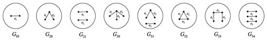
Figure 1. The graphs obtained by removing up to three edges from a complete graph $K_n$.

By Theorem 1, we can obtain some properties of second signless Laplacian immanantal polynomials of graphs.

Lemma 6.

From the second signless Laplacian immanantal polynomial of a graph G, we can derive:

(i) 

n, the vertex count;

(ii) 

m, the edge count;

(iii) 

${\sum }_{1\le i\le n}{d}_i^2$, the sum of the squares of the vertex degrees.

Proof. 

By Theorem 1, it can be inferred that the coefficients $c_0\left(G\right),c_1\left(G\right)$ of the second signless Laplacian immanantal polynomial of graph G can be used to derive the number of vertices and edges of graph G, where

$$\begin{array}{ccc}\hfill c_2\left(G\right)& =& (n-1)a_2\left(G\right)-m(n-3)(n⩾3),\hfill \\ \hfill a_2\left(G\right)& =& \sum _{1\le i<j\le n}{d}_i{d}_j={\displaystyle \frac{1}{2}}[{(\sum _{i=1}^n{d}_i)}^2-\sum _{i=1}^n{d}_i^2]=2m^2-{\displaystyle \frac{1}{2}}\sum _{i=1}^n{d}_i^2.\hfill \end{array}$$

The coefficients $c_2\left(G\right)$ of the second signless Laplacian immanantal polynomial of graph G can be used to derive the sum of squares of the vertex degrees of graph G. □

The reference [25] provides the results of the sum of squares of the vertex degrees for some graphs, as shown in Table 1.

Table 1. The sum of squares of the vertex degrees of some graphs in ${\mathcal{G}}_n$.

Graph G	${\sum }_{1\le \mathit{i}\le \mathit{n}}{\mathit{d}}_{\mathit{i}}^2$
$G_{20}$	$n^3-2n^2-7n+14$
$G_{21}$	$n^3-2n^2-7n+12$
$G_{30},G_{32}$	$n^3-2n^2-11n+24$
$G_{31}$	$n^3-2n^2-11n+20$
$G_{33}$	$n^3-2n^2-11n+22$
$G_{34}$	$n^3-2n^2-11n+18$

Theorem 9.

The graphs obtained by removing up to three edges from a complete graph $K_n$ are determined by the second signless Laplacian immanantal polynomial.

Proof. 

By Lemma 6 and Table 1, Graphs $G_{10},G_{20},G_{21},G_{31},G_{33},G_{34}$ are determined by the second signless Laplacian immanantal polynomial, respectively. And

$$\sum _{1\le i\le n}{d}_i^2\left(G_{30}\right)=\sum _{1\le i\le n}{d}_i^2\left(G_{32}\right)=n^3-2n^2-11n+24,$$

and by Theorem 1,

$$\begin{array}{ccc}\hfill a_3\left(G\right)& =& {\displaystyle \frac{1}{6}}[(\sum _{i=1}^n{d}_i{)}^3-\sum _{i=1}^n{d}_i^3-3\sum _{i=1}^n\sum _{\begin{array}{c}j=1\\ j\ne i\end{array}}^n{d}_i{d}_j^2]\hfill \\ & =& {\displaystyle \frac{4}{3}}{m}^3-{\displaystyle \frac{1}{6}}\sum _{i=1}^n{d}_i^3-{\displaystyle \frac{1}{2}}[(\sum _{i=1}^n{d}_i)(\sum _{j=1}^n{d}_j^2)-\sum _{i=1}^n{d}_i^3]\hfill \\ & =& {\displaystyle \frac{4}{3}}{m}^3+{\displaystyle \frac{1}{3}}\sum _{i=1}^n{d}_i^3-m\sum _{i=1}^n{d}_i^2.\hfill \end{array}$$

According to reference [6], $b_3\left(G\right)=2m^2-{\sum }_{i=1}^n{d}_i^2$; according to reference [25], $T\left(G_{30}\right)=\left({\displaystyle \genfrac{}{}{0pt}{}{n}{3}}\right)-3n+9,T\left(G_{32}\right)=\left({\displaystyle \genfrac{}{}{0pt}{}{n}{3}}\right)-3n+8$. Then

$$\begin{array}{ccc}& & c_3\left(G_{30}\right)-c_3\left(G_{32}\right)\hfill \\ & =& (n-1)·{\displaystyle \frac{1}{3}}[\sum _{i=1}^n{d}_i^3\left(G_{32}\right)-\sum _{i=1}^n{d}_i^3\left(G_{30}\right)]+2(n-4)(T\left(G_{30}\right)-T\left(G_{32}\right))=-6.\hfill \end{array}$$

This means that the graphs $G_{30}$ and $G_{32}$ are determined by the second signless Laplacian immanantal polynomial. The theorem is proved. □

4. Conclusions

This paper established fundamental algebraic and spectral properties of the second signless Laplacian immanantal polynomial of a graph. Explicit formulas for its first five coefficients are derived, inequalities involving specific coefficients are established, and the distribution of its roots is described. Furthermore, the question posed by van Dam and Haemers [23] of whether a graph is determined by its characteristic polynomial motivates the study of various polynomials for graph characterization. We prove an equivalence between the characteristic polynomial and the second signless Laplacian immanantal polynomial for regular graphs: if two regular graphs have the same characteristic polynomial, then they also share the same second signless Laplacian immanantal polynomial. For non-regular graphs, sufficient conditions for a graph to be determined by this polynomial are provided, and it is shown that certain special graph classes are uniquely determined by it. There are relatively few research results related to immanantal polynomials, and many challenging open problems warrant further investigation. For example, the second signless Laplacian immanantal polynomial characterization or real root characterization of general graph classes.

References

- Ramane, H.S.; Gudimani, S.B.; Shinde, S.S. Signless Laplacian polynomial and characteristic polynomial of a graph. Discret. Math. 2013, 1, 105624. [Google Scholar] [CrossRef]
- Agrawal, M. Determinant versus permanent. In Proceedings of the International Congress of Mathematicians, Madrid, Spain, 22–30 August 2006; European Mathematical Society-EMS-Publishing House GmbH: Berlin, Germany, 2007. [Google Scholar]
- Wu, T.; Luo, J.; Gao, Y. On the permanent indices of graphs. Appl. Math. Comput. 2026, 516, 129883. [Google Scholar] [CrossRef]
- Liu, S. On the (signless) Laplacian permanental polynomials of graphs. Graphs Comb. 2019, 35, 787–803. [Google Scholar] [CrossRef]
- Zhang, H.; Wu, T.; Lai, H. Per-spectral characterizations of some edge-deleted subgraphs of a complete graph. Linear Multilinear Algebra 2015, 63, 397–410. [Google Scholar] [CrossRef]
- Merris, R. The second immanantal polynomial and the centroid of a graph. SIAM J. Algebr. Discret. Methods 1986, 7, 484–503. [Google Scholar] [CrossRef]
- Biggs, N. Algebraic Graph Theory; Cambridge University Press: Cambridge, MA, USA, 1993. [Google Scholar]
- Hou, Y.; Lei, T. Characteristic polynomials of skew-adjacency matrices of oriented graphs. Electron. J. Comb. 2011, 18, P156. [Google Scholar] [CrossRef]
- Zhang, X.; Luo, R. The Laplacian eigenvalues of mixed graphs. Linear Algebra Appl. 2003, 362, 109–119. [Google Scholar] [CrossRef]
- Brualdi, R.A.; Goldwasser, J.L. Permanent of the Laplacian matrix of trees and bipartite graphs. Discrete Math. 1984, 48, 1–21. [Google Scholar] [CrossRef]
- Botti, P.; Merris, R.; Vega, C. Laplacian permanents of trees. SIAM J. Discret. Math. 1992, 5, 460–466. [Google Scholar] [CrossRef]
- Faria, I. Permanental roots and star degree of a graph. Linear Algebra Appl. 1985, 64, 255–265. [Google Scholar] [CrossRef]
- Bapat, R.B. A bound for the permanent of the Laplacian matrix. Linear Algebra Appl. 1986, 74, 219–223. [Google Scholar] [CrossRef]
- Wu, T.; Yu, Y.; Feng, L.; Gao, X. On the second immanantal polynomials of graphs. Discrete Math. 2024, 347, 114105. [Google Scholar] [CrossRef]
- Wu, T.; Yu, Y.; Gao, X. The second immanantal polynomials of Laplacian matrices of unicyclic graphs. Appl. Math. Comput. 2023, 451, 128038. [Google Scholar] [CrossRef]
- Bürgisser, P. The computational complexity of immanants. SIAM J. Comput. 2000, 30, 1023–1040. [Google Scholar] [CrossRef]
- Cash, G.G. Immanants and Immanantal Polynomials of Chemical Graphs. J. Chem. Inf. Comput. Sci. 2003, 43, 1942–1946. [Google Scholar] [CrossRef]
- Chan, O.; Lam, T. Immanant inequalities for Laplacians of trees. SIAM J. Matrix Anal. Appl. 1999, 21, 129–144. [Google Scholar] [CrossRef]
- Chan, O.; Lam, T.; Merris, R. Wiener number as an immanant of the Laplacian of molecular graphs. J. Chem. Inf. Comput. Sci. 1997, 37, 762–765. [Google Scholar] [CrossRef]
- Merris, R. Immanantal invariants of graphs. Linear Algebra Appl. 2005, 401, 67–75. [Google Scholar] [CrossRef][Green Version]
- Botti, P.; Merris, R. Almost all trees share a complete set of immanantal polynomials. J. Graph Theory 1993, 17, 467–476. [Google Scholar] [CrossRef]
- Yu, G.; Qu, H. The coefficients of the immanantal polynomial. Appl. Math. Comput. 2018, 339, 38–44. [Google Scholar] [CrossRef]
- van Dam, E.R.; Haemers, W.H. Which graphs are determined by their spectrum? Linear Algebra Appl. 2003, 373, 241–272. [Google Scholar] [CrossRef]
- van Dam, E.R.; Haemers, W.H. Developments on spectral characterizations of graphs. Discrete Math. 2009, 309, 576–586. [Google Scholar] [CrossRef]
- Wu, T.; Zhou, T. The characterizing properties of (signless) laplacian permanental polynomials of almost complete graphs. J. Math. 2021, 2021, 9161508. [Google Scholar] [CrossRef]
Disclaimer/Publisher’s Note: The statements, opinions and data contained in all publications are solely those of the individual author(s) and contributor(s) and not of MDPI and/or the editor(s). MDPI and/or the editor(s) disclaim responsibility for any injury to people or property resulting from any ideas, methods, instructions or products referred to in the content. |
© 2026 by the authors. Licensee MDPI, Basel, Switzerland. This article is an open access article distributed under the terms and conditions of the Creative Commons Attribution (CC BY) license.