A Note on Chaos of a Modified Piecewise Linear Discontinuous System with Multiple-Well Potentials: Melnikov Approach with Simulations

Abstract

The topic of chaotic thresholds for piecewise linear discontinuous (PWLD) systems with multiple-well potentials is a persistent topic in the research of a number of authors. In this article we investigate the chaos of a modified piecewise linear discontinuous (MPWLD) system. The model, containing N free parameters, could be of interest to specialists working in this area. With a specially developed software product, we generate the Melnikov equation $M\left(t\right)=0$ and examine all its zeros. This opens up an opportunity for researchers to correctly understand and formulate the classical Melnikov criterion for the possible occurrence of chaos in dynamical systems. Several simulations are composed. We also demonstrate some specialized modules for investigating the dynamics of the proposed model. Intriguing and new generalizations made through probabilistic constructions are considered.

1. Introduction

Studies on the equilibrium bifurcation problem of non-smooth systems were first reported in 1949 by Andronov [1].

It is well known that piecewise linear systems are typical non-smooth dynamics systems that often occur in engineering and science [2,3,4,5,6].

Various types of discontinuous dynamical systems [7] have been studied in the literature, including the Filippov-type discontinuity; the discontinuous right-hand side [8]; dry friction dampers [9,10]; phase-state discontinuities, such as impacting systems [11,12]; and also systems with a non-smooth Jacobian matrix [13,14].

Many authors devote their research to this interesting topic.

The detection of grazing orbits and incident bifurcations of a forced continuous piecewise linear oscillator is considered by Hu [15].

Bernardo and Hogan [16] present an overview of the discontinuity-induced bifurcations of piecewise smooth dynamical systems.

Canards in piecewise linear system explosions and super-explosions can be found in [17].

Archetypal oscillators for smooth and discontinuous dynamics are discussed in [18,19].

Chaotic oscillations in a piecewise linear spring–mass system are considered in [20].

For a bifurcation analysis of a smooth-and-discontinuous oscillator, see [21,22,23].

The chaotic behavior of oscillators with strong irrational nonlinearities and second-order piecewise linear systems is considered in [24,25,26].

The reader can find interesting considerations about Melnikov functions for singularly perturbed ordinary differential equations in [27].

These studies range from theoretical formulations and methodologies to applications in engineering science.

Ref. [28] shows that some knowledge of differential equations can be generalized for discontinuous systems.

The most attention has been focused on planar systems with a homoclinic trajectory that have been perturbed by a periodic function. It was proved, under additional assumptions, that this perturbed system has a homoclinic solution again.

The proof is based on the existence of simple zeroes of a “non-smooth” Melnikov function.

It was shown [28] that if we want to use the Melnikov method, we need the existence and continuity of the second derivative of the right-hand side out of the discontinuity surface.

More precisely, Kukuchka [28] also notes the following: “…For example, we could consider other perturbations instead of periodic ones or we could deal with the Melnikov method for systems in $R^n$, $n\ge 2$, but the most interesting case would be to remove the restriction of transversal intersections through the discontinuity surface. This should be an initiative for the next study.”.

Detailed information on other difficulties that researchers encounter in the direct application of Melnikov’s theory can be found in the monographic study in [29].

For other results, see [30,31].

Many studies on friction oscillator models, semi-dynamical systems, and other mechanisms are based on Filippov regularization. For more details, see [32,33,34,35,36,37].

In [38], the authors consider the following piecewise linear discontinuous system with multiple-well potentials:

$$\left\{\begin{array}{ccc}{\displaystyle \frac{\mathrm{d}x}{\mathrm{d}t}}\hfill & =& y,\hfill \\ {\displaystyle \frac{\mathrm{d}y}{\mathrm{d}t}}\hfill & =& -2x+\mathrm{sign}(x+\alpha )+\mathrm{sign}(x-\alpha )-ϵ\left(ay-fcos\left(\omega t\right)\right).\hfill \end{array}\right.$$

(1)

With the help of the Hamiltonian function ($ϵ=0$), the authors study all special homo–heteroclinic-like orbits [38]:

$$(x_{\pm }^1\left(t_1\right),y_{\pm }^1\left(t_1\right))=\left\{(\pm 1\pm cos\sqrt{2}{t}_1,\mp \sqrt{2}sin\sqrt{2}{t}_1)\right\}\cup \left\{(0,0)\right\}$$

for $t_1\in \left(-{\displaystyle \frac{\pi }{\sqrt{2}}},{\displaystyle \frac{\pi }{\sqrt{2}}}\right)$;

$$(x_{\pm }^2\left(t_1\right),y_{\pm }^2\left(t_1\right))=\left\{(\pm 1\pm (1-\alpha )cos\sqrt{2}{t}_1,\mp (1-\alpha )\sqrt{2}sin\sqrt{2}{t}_1)\right\}\cup \left\{(\pm \alpha ,0)\right\}$$

for $t_1\in \left(-{\displaystyle \frac{\pi }{\sqrt{2}}},{\displaystyle \frac{\pi }{\sqrt{2}}}\right)$;

$$(x_{\pm }^3\left(t_2\right),y_{\pm }^3\left(t_2\right))=\left\{(\pm \alpha sin\sqrt{2}{t}_2,\pm \alpha \sqrt{2}cos\sqrt{2}{t}_2)\right\}\cup \left\{(\pm \alpha ,0)\right\}$$

for $t_2\in \left(-{\displaystyle \frac{\pi }{2\sqrt{2}}},{\displaystyle \frac{\pi }{2\sqrt{2}}}\right)$;

$$(x_{\pm }^4\left(t_2\right),y_{\pm }^4\left(t_2\right))=\left\{(\pm sin\sqrt{2}{t}_2,\pm \sqrt{2}cos\sqrt{2}{t}_2)\right\}\cup \left\{(\pm 1,0)\right\}$$

for $t_2\in \left(-{\displaystyle \frac{\pi }{2\sqrt{2}}},{\displaystyle \frac{\pi }{2\sqrt{2}}}\right)$.

The Melnikov criterion for generating chaos in system (1) is also discussed.

In this paper we consider a generalization of differential system (1).

We study chaos in the proposed new model.

Several simulations are composed. We also demonstrate some specialized modules for investigating the dynamics of the model.

Intriguing generalizations made through probabilistic constructions are considered.

2. A New Generalized Model: Melnikov Approach

We consider the new modified dynamical system of the form:

$$\left\{\begin{array}{ccc}{\displaystyle \frac{\mathrm{d}x}{\mathrm{d}t}}\hfill & =& y,\hfill \\ {\displaystyle \frac{\mathrm{d}y}{\mathrm{d}t}}\hfill & =& -2x+\mathrm{sign}(x+\alpha )+\mathrm{sign}(x-\alpha )-ϵ\left(Ay-{\displaystyle \sum _{j=1}^N}{g}_{j}cos\left(j\omega t\right)\right),\hfill \end{array}\right.$$

(2)

where $0\le ϵ<1$, A is the damping level, $g_i\ge 0;i=1,\dots ,N$, and N is integer.

The Melnikov function [39] gives a measure of the leading-order distance between the stable and unstable manifolds when $ϵ\ne 0$ and can be used to tell where the stable and unstable manifolds intersect transversely.

By definition, the Melnikov integral is given by

$$\begin{array}{ccc}{M}_{\pm }^i\left(t_0\right)\hfill & =& {\displaystyle {\int }_{-\infty }^{\infty }}\left(-A{\left(y_{\pm }^i\left(t\right)\right)}^2+y_{\pm }^i\left(t\right){\displaystyle \sum _{j=1}^N}{g}_{j}cos\left(j\omega (t+t_0)\right)\right)\mathrm{d}t,i=1,2,3,4.\hfill \end{array}$$

(3)

From a numerical point of view, the task of finding all roots of $M_{\pm }^i\left(t_0\right)$, $i=1,2,3,4$ is interesting, given that the parameters appearing in the proposed differential model are subject to a number of restrictions of a physical and practical nature.

We can prove the following proposition when $N=2$.

Proposition 1.

If $N=2$, then the roots of the Melnikov function $M_{\pm }^i\left(t_0\right)$, $i=1,2,3,4$, are given as solutions of the following equations:

$$\begin{array}{ccc}{M}_{+}^1\left(t_0\right)\hfill & =& -\sqrt{2}A\pi +{\displaystyle \frac{4g_{1}sin\left(\frac{\pi \omega }{\sqrt{2}}\right)}{-2+{\omega }^2}}sin\left(t_0\omega \right)+{\displaystyle \frac{2g_{2}sin\left(\sqrt{2}\pi \omega \right)}{-1+2{\omega }^2}}sin\left(2t_0\omega \right)=0;\hfill \\ M_{+}^2\left(t_0\right)\hfill & =& -\sqrt{2}A\pi {(-1+\alpha )}^2+(-1+\alpha )\left({\displaystyle \frac{4g_{1}sin\left(\frac{\pi \omega }{\sqrt{2}}\right)}{-2+{\omega }^2}}sin\left(t_0\omega \right)\right.\hfill \\ \hfill & & \left.+{\displaystyle \frac{2g_{2}sin\left(\sqrt{2}\pi \omega \right)}{-1+2{\omega }^2}}sin\left(2t_0\omega \right)\right)=0;\hfill \\ M_{-}^3\left(t_0\right)\hfill & =& -{\displaystyle \frac{A\pi {\alpha }^2}{\sqrt{2}}}+{\displaystyle \frac{4g_1\alpha cos\left(\frac{\pi \omega }{2\sqrt{2}}\right)}{-2+{\omega }^2}}cos\left(t_0\omega \right)+{\displaystyle \frac{2g_2\alpha cos\left(\frac{\pi \omega }{\sqrt{2}}\right)}{-1+2{\omega }^2}}cos\left(2t_0\omega \right)=0;\hfill \\ M_{-}^4\left(t_0\right)\hfill & =& -{\displaystyle \frac{A\pi }{\sqrt{2}}}+{\displaystyle \frac{4g_{1}cos\left(\frac{\pi \omega }{2\sqrt{2}}\right)}{-2+{\omega }^2}}cos\left(t_0\omega \right)+{\displaystyle \frac{2g_{2}cos\left(\frac{\pi \omega }{\sqrt{2}}\right)}{-1+2{\omega }^2}}cos\left(2t_0\omega \right)=0.\hfill \end{array}$$

(4)

For example, the Melnikov function $M_{-}^4\left(t_0\right)$ for $N=2$ in case (A), $A=0.009$, $\omega =0.879$, $g_1=0.09$, $g_2=0.16$, is depicted in Figure 1. (In this case, the Melnikov function is a trigonometric polynomial that has two simple zeros in the considered interval).

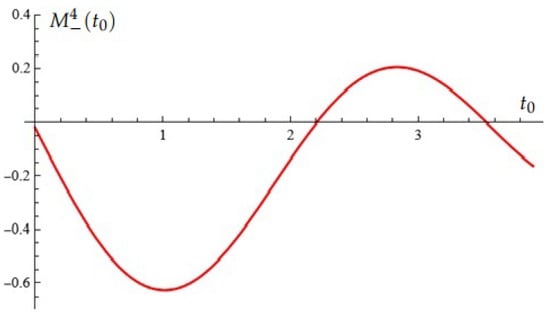
Figure 1. Equation $M_{-}^4\left(t_0\right)=0$ (Proposition 1); case (A).

Case (B): $A=0.006$, $\omega =0.08$, $g_1=0.39$, $g_2=0.26$. In this case, the Melnikov polynomial has root $t_0=3.11969$ with multiplicity two (see Figure 2).

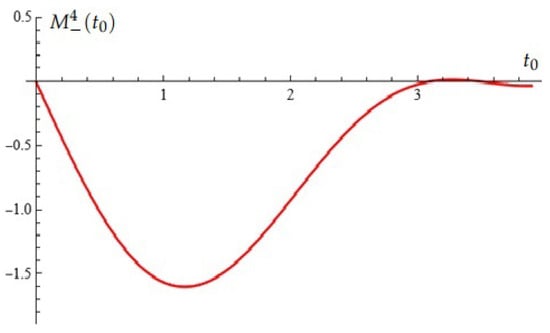
Figure 2. Equation $M_{-}^4\left(t_0\right)=0$ (Proposition 1); case (B).

We can prove the following proposition when $N=3$.

Proposition 2.

If $N=3$, then the roots of the Melnikov function $M_{-}^3\left(t_0\right)$ are given as solutions of the following equation:

$$\begin{array}{ccc}{M}_{-}^3\left(t_0\right)\hfill & =& -{\displaystyle \frac{A\pi {\alpha }^2}{\sqrt{2}}}+{\displaystyle \frac{4\alpha g_{1}cos\left(\frac{\pi \omega }{2\sqrt{2}}\right)}{-2+{\omega }^2}}cos\left(t_0\omega \right)+{\displaystyle \frac{2g_2\alpha cos\left(\frac{\pi \omega }{\sqrt{2}}\right)}{-1+2{\omega }^2}}cos\left(2t_0\omega \right)\hfill \\ \hfill & & +{\displaystyle \frac{4g_3\alpha cos\left(\frac{3\pi \omega }{2\sqrt{2}}\right)}{-2+9{\omega }^2}}cos\left(3t_0\omega \right)=0.\hfill \end{array}$$

(5)

For example, the Melnikov function $M_{-}^3\left(t_0\right)$ for $N=3$, $\alpha =0.5$ in case (A), $A=0.009$, $\omega =0.879$, $g_1=0.09$, $g_2=0.16$, $g_3=0.3$, is depicted in Figure 3. (In this case the Melnikov polynomial has three simple zeros.)

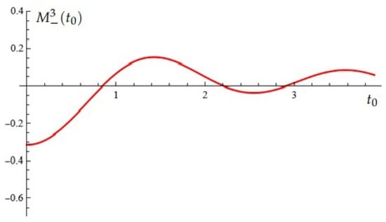
Figure 3. Equation $M_{-}^3\left(t_0\right)=0$ (Proposition 2); case (A).

Case (B): $A=0.005$, $\omega =0.9$, $g_1=0.135$, $g_2=0.21$, $g_3=0.3$. In this case the Melnikov polynomial has one simple zero and root $t_0\approx 2.52$ with multiplicity two (see Figure 4).

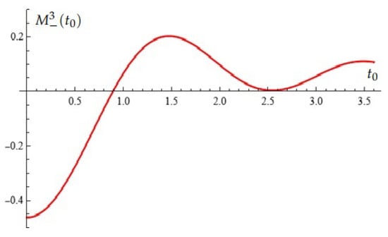
Figure 4. Equation $M_{-}^3\left(t_0\right)=0$ (Proposition 2); case (B).

Melnikov criterion. If $M\left(t_0\right)=0$ and ${\displaystyle \frac{\mathrm{d}M\left(t_0\right)}{\mathrm{d}{t}_0}}\ne 0$ for some $t_0$ and some sets of parameters, then this indicates the possibility of chaotic dynamics under the stated assumptions.

From Propositions 1 and 2, the reader may formulate the Melnikov criterion for the intersection of projections of separatrixes onto the phase plane and possibly chaos.

3. Some Simulations

We will look at some interesting simulations using model (2):

Example 1.

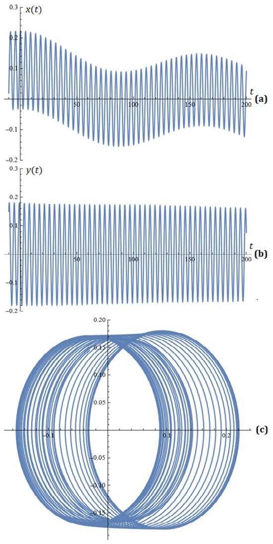
For $N=4$, $\alpha =0.95$, $A=0.01$, $\omega =0.01$, $g_1=0.6$, $g_2=0.2$, $g_3=0.3$, $g_4=0.8$, $ϵ=0.1$, the simulations on system (2) for $x_0=0.2$, $y_0=0.1$ are depicted in Figure 5.

Figure 5. (a) x-component of the solutions of system (2); (b) y-component of the solutions of system (2); (c) phase space (Example 1).

Example 2.

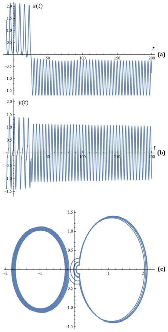
For $N=6$, $\alpha =0.15$, $A=0.01$, $\omega =0.01$, $g_1=0.6$, $g_2=0.2$, $g_3=0.3$, $g_4=0.8$, $g_5=0.1$, $g_6=0.7$, $ϵ=0.1$, the simulations on system (2) for $x_0=0.1$, $y_0=0.1$ are depicted in Figure 6.

Figure 6. (a) x-component of the solutions of system (2); (b) y-component of the solutions of system (2); (c) phase space (Example 2).

Example 3.

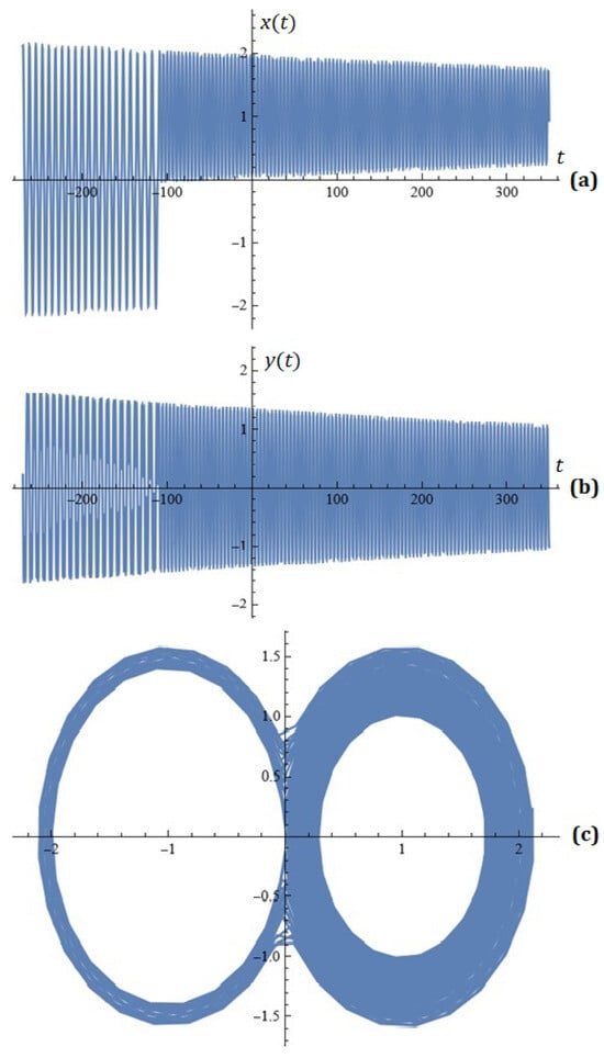
For $N=7$, $\alpha =0.01$, $A=0.07$, $\omega =0.01$, $g_1=0.01$, $g_2=0.12$, $g_3=0.2$, $g_4=0.4$, $g_5=0.1$, $g_6=0.1$, $g_7=0.5$, $ϵ=0.02$, the simulations on system (2) for $x_0=0.1$, $y_0=-0.1$ are depicted in Figure 7.

Figure 7. (a) x-component of the solutions of system (2); (b) y-component of the solutions of system (2); (c) phase space (Example 3).

Example 4.

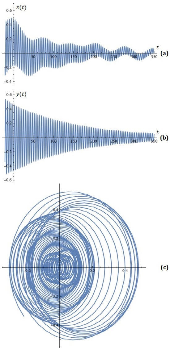
For $N=9$, $\alpha =0.95$, $A=0.07$, $\omega =0.01$, $g_1=0.06$, $g_2=0.12$, $g_3=0.3$, $g_4=0.18$, $g_5=0.1$, $g_6=0.2$, $g_7=0.3$, $g_8=0.05$, $g_9=0.4$, $ϵ=0.18$, the simulations on system (2) for $x_0=0.4$, $y_0=0.3$ are depicted in Figure 8.

Figure 8. (a) x-component of the solutions of system (2); (b) y-component of the solutions of system (2); (c) phase space (Example 4).

Example 5.

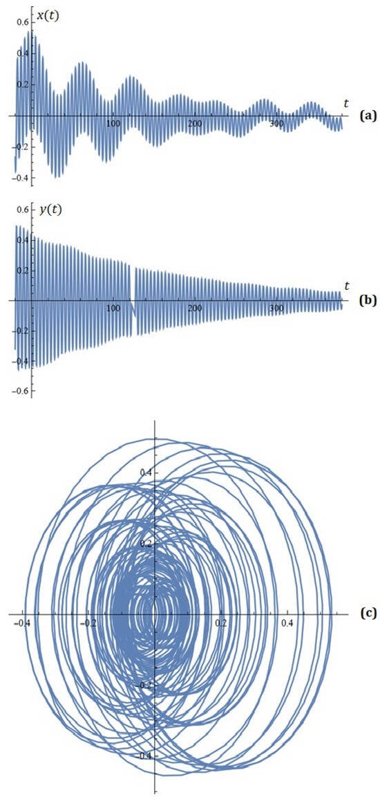
For $N=11$, $\alpha =0.97$, $A=0.1$, $\omega =0.01$, $g_1=0.3$, $g_2=0.15$, $g_3=0.05$, $g_4=0.25$, $g_5=0.15$, $g_6=0.25$, $g_7=0.1$, $g_8=0.1$, $g_9=0.9$, $g_{10}=0.95$, $g_{11}=1.05$, $ϵ=0.107$, the simulations on system (2) for $x_0=0.45$, $y_0=0.3$ are depicted in Figure 9.

Figure 9. (a) x-component of the solutions of system (2); (b) y-component of the solutions of system (2); (c) phase space (Example 5).

The reader can also consider other interesting examples that demonstrate the variety of phase portraits depending on the variation of the parameter $\alpha$ in the considered interval $[0,1]$, and for this reason we will not dwell on these demonstrations here.

4. Further Generalizations Through Probabilistic Constructions

Let us slightly modify model (2) by changing the $\mathrm{sign}$ function with the indicator function $2I_{x\ge 0}-1$:

$$\begin{array}{cc}\hfill {\displaystyle \frac{\mathrm{d}x}{\mathrm{d}t}}& =y,\hfill \\ \hfill {\displaystyle \frac{\mathrm{d}y}{\mathrm{d}t}}& =2\left(I_{x\ge -\alpha }+I_{x\ge \alpha }-x-1\right)-ϵ\left(Ay-\sum _{j=1}^N{g}_{j}cos\left(j\omega t\right)\right).\hfill \end{array}$$

(6)

We shall now generalize model (6) in two directions. First, let the function $G\left(·\right)$ stand for the step part:

$$G\left(x\right)=I_{x\ge -\alpha }+I_{x\ge \alpha }.$$

(7)

Its behavior (for $\alpha =1$) can be seen in Figure 10a. One can recognize the double cumulative distribution function (CDF) of a distribution with atoms in the points $-\alpha$ and $\alpha$ with probabilities ${\displaystyle \frac{1}{2}}$. Hence, we can generalize the dynamics (6) by using an arbitrary distribution with CDF $F\left(·\right)$, as well as different weights for the non-perturbed terms:

$$\begin{array}{cc}\hfill {\displaystyle \frac{\mathrm{d}x}{\mathrm{d}t}}& =y,\hfill \\ \hfill {\displaystyle \frac{\mathrm{d}y}{\mathrm{d}t}}& =b_{1}F\left(x\right)-b_{2}x-b_3-ϵ\left(Ay-\sum _{j=1}^N{g}_{j}cos\left(j\omega t\right)\right).\hfill \end{array}$$

(8)

The importance of generalization (8) is in several directions. On one hand, introduction of the coefficients $b_1$, $b_2$, and $b_3$ is a more or less technical assumption but it gives the user more flexibility. Note that the term $-x-1$ in (6) is a downward compensator whose force can be controlled through $b_1$, $b_2$, and $b_3$ in (8). On the other hand, the most important factor is the CDF that replaces the indicator part (7). In the original model (6), the indicators play the role of a jump impulse from one state to another for the derivative of the y-component with respect to the position of the x-term (with respect to $\pm \alpha$). Thus, by introducing a CDF which combines a continuous part with atoms, we can incorporate a suitable continuous dependence of the y-derivative between the jumps that occur in the atoms. Also, the probability at an atom gives the jump size for the y-derivative at this place.

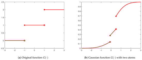
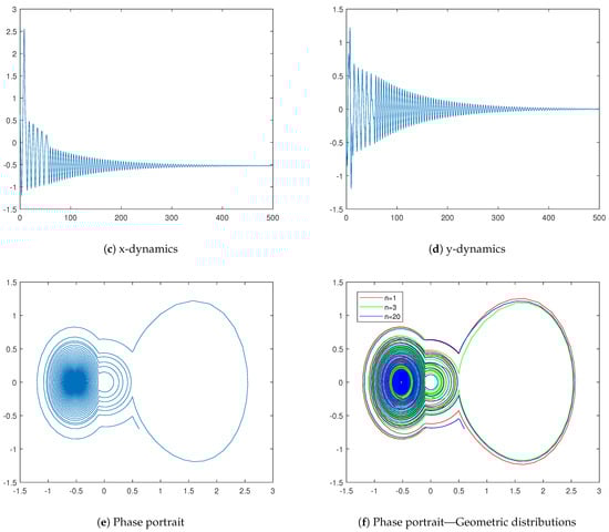
Figure 10. Oscillators based on the Exponential distribution.

We can generalize further using the complex presentation of the cos function:

$$cos\left(x\right)={\displaystyle \frac{e^{ix}+e^{-ix}}{2}}.$$

(9)

Let ${\displaystyle K=\sum _{k=1}^N{g}_k}$ and ${\overline{g}}_j={\displaystyle \frac{g_j}{K}}$. Let $\xi$ be a random variable distributed on the set $\left\{1,2,\dots ,N\right\}$ with probabilities ${\overline{g}}_k$. Let its characteristic function be denoted by $\psi \left(x\right)$. We can rewrite the y-dynamics of (6) as

$$\begin{array}{cc}\hfill {\displaystyle \frac{\mathrm{d}y}{\mathrm{d}t}}& =b_{1}F\left(x\right)-b_{2}x-b_3-ϵK\left(Ay-\sum _{k=1}^N{\overline{g}}_{k}cos\left(k\omega t\right)\right)\hfill \\ \hfill & =b_{1}F\left(x\right)-b_{2}x-b_3-ϵK\left(Ay-\sum _{k=1}^N{\overline{g}}_k{\displaystyle \frac{e^{ik\omega t}+e^{-ik\omega t}}{2}}\right)\hfill \\ \hfill & =b_{1}F\left(x\right)-b_{2}x-b_3-ϵK\left(Ay-{\displaystyle \frac{\mathbb{E}\left[e^{i\omega t\xi }\right]+\mathbb{E}\left[e^{-i\omega t\xi }\right]}{2}}\right)\hfill \\ \hfill & =b_{1}F\left(x\right)-b_{2}x-b_3-ϵK\left(Ay-{\displaystyle \frac{1}{2}}\left(\psi \left(\omega t\right)+\psi \left(-\omega t\right)\right)\right),\hfill \end{array}$$

(10)

where $\mathbb{E}$ stands for the mathematical expectation. We can use an arbitrary random variable distributed on a domain D instead of the set $\left\{1,2,\dots ,N\right\}$. This way, the sum in dynamics (6) should be changed into an integral:

$${\displaystyle \frac{\mathrm{d}y}{\mathrm{d}t}}=b_{1}F\left(x\right)-b_{2}x-b_3-ϵK\left(Ay-\underset{D}{\int }cos\left(u\omega t\right)g\left(\mathrm{d}u\right)\right),$$

(11)

where $g\left(·\right)$ is the density function. Thus, we transform the original dynamics (2) into

$$\begin{array}{cc}\hfill {\displaystyle \frac{\mathrm{d}x}{\mathrm{d}t}}& =y,\hfill \\ \hfill {\displaystyle \frac{\mathrm{d}y}{\mathrm{d}t}}& =b_{1}F\left(x\right)-b_{2}x-b_3-ϵK\left(Ay-{\displaystyle \frac{1}{2}}\left(\psi \left(\omega t\right)+\psi \left(-\omega t\right)\right)\right).\hfill \end{array}$$

(12)

Having in mind this presentation, we rewrite Melnikov integral (3) as

$$\begin{array}{cc}\hfill M_{\pm }^i\left(t_0\right)& ={\int }_{-\infty }^{\infty }\left(-A{\left(y_{\pm }^i\left(t\right)\right)}^2+{\displaystyle \frac{y_{\pm }^i\left(t\right)}{2}}\left(\psi \left(\omega \left(t+t_0\right)\right)+\psi \left(-\omega \left(t+t_0\right)\right)\right)\right)\mathrm{d}t,\hfill \\ \hfill & i=1,2,3,4.\hfill \end{array}$$

(13)

Let us discuss an example for which the random variable that drives the perturbations is exponentially distributed and thus its characteristic function is

$$\psi \left(x\right)={\displaystyle \frac{\beta }{\beta -ix}}.$$

(14)

Hence,

$$\psi \left(x\right)+\psi \left(-x\right)=2{\displaystyle \frac{{\beta }^2}{{\beta }^2+x^2}}.$$

(15)

Thus, dynamics (12) turns into

$$\begin{array}{cc}\hfill {\displaystyle \frac{\mathrm{d}x}{\mathrm{d}t}}& =y,\hfill \\ \hfill {\displaystyle \frac{\mathrm{d}y}{\mathrm{d}t}}& =b_{1}F\left(x\right)-b_{2}x-b_3-ϵK\left(Ay-{\displaystyle \frac{{\beta }^2}{{\beta }^2+{\omega }^2{t}^2}}\right),\hfill \end{array}$$

(16)

whereas Melnikov integral (13) is

$$\begin{array}{cc}\hfill M_{\pm }^i\left(t_0\right)& ={\int }_{-\infty }^{\infty }\left(-A{\left(y_{\pm }^i\left(t\right)\right)}^2+y_{\pm }^i\left(t\right){\displaystyle \frac{{\beta }^2}{{\beta }^2+{\omega }^2{\left(t+t_0\right)}^2}}\right)\mathrm{d}t,i=1,2,3,4.\hfill \end{array}$$

(17)

Unfortunately, Melnikov integral (17) cannot be evaluated through closed-form formulas and thus some numerical methods have to be applied.

We continue with our example considering the following CDF $F\left(·\right)$ that combines a Gaussian function and atoms:

$$F\left(x\right)=\left\{\begin{array}{c}{c}_{1}N\left(x\right),x<{\alpha }_1\hfill \\ c_{2}N\left(x\right),x\in \left[{\alpha }_1,{\alpha }_2\right)\hfill \\ N\left(x\right),x\ge {\alpha }_2,\hfill \end{array}\right.$$

(18)

where $0<c_1<c_2<1$ and $N\left(x\right)$ is the CDF of the standard normal distribution:

$$N\left(x\right)={\displaystyle \frac{1}{\sqrt{2\pi }}}\underset{-\infty }{\overset{x}{\int }}{e}^{-{\displaystyle \frac{u^2}{2}}}\mathrm{d}u.$$

(19)

Function (18) is depicted in Figure 10b for the following values of the parameters: ${\alpha }_1=-0.1$, ${\alpha }_2=0.5$, $c_1=0.3$, and $c_2=0.6$.

The behavior of this oscillator is presented in Figure 10c (x-dynamics), Figure 10d (y-dynamics), and Figure 10e (phase portrait). In addition to the above-applied parameters, we use $b_1=5$, $b_2=2$, $b_3=1.5$, $ϵ=0.1$, $K=1$, $A=0.2$, $\omega =1.01$, $\beta =0.3$, $x_0=0.6$, and $y_0=-0.7$.

Last but not least, we shall discuss the perturbation term in dynamics (12). We can observe that the periodicity vanishes for the exponential distribution—see system (16). It turns out that this is due to some convergence reasons. To confirm this, we shall consider the exponential distribution as a limit of a sequence of suitable geometric distributions. For every $n>\beta$, let ${\xi }_n$ be a geometrically distributed random variable with the success rate $p_n={\displaystyle \frac{\beta }{n}}$ and let the random variable ${\eta }_n$ be defined as ${\eta }_n={\displaystyle \frac{{\xi }_n}{n}}$. We can observe for the cumulative distribution function when n tends to infinity:

$$\underset{n\to \infty }{lim}\mathbb{P}\left({\eta }_n<x\right)=\underset{n\to \infty }{lim}\mathbb{P}\left({\xi }_n<nx\right)=\underset{n\to \infty }{lim}1-{\left(1-{\displaystyle \frac{\beta }{n}}\right)}^{\left[nx\right]}=1-e^{-\beta x}.$$

(20)

Above, we denote by $\left[x\right]$ the integer part of x. One can recognize the cumulative distribution function of the exponential distribution in the last term of (20). Let us consider a geometric distribution with success rate p for the perturbation term of dynamics (12). We can easily derive

$$\begin{array}{cc}\hfill {\displaystyle \frac{\psi \left(x\right)+\psi \left(-x\right)}{2}}& ={\displaystyle \frac{p}{2}}\left[{\displaystyle \frac{e^{ix}}{1-\left(1-p\right)e^{ix}}}+{\displaystyle \frac{e^{-ix}}{1-\left(1-p\right)e^{-ix}}}\right]\hfill \\ \hfill & =p{\displaystyle \frac{cos\left(x\right)-1+p}{1+{\left(1-p\right)}^2-2\left(1-p\right)cos\left(x\right)}}.\hfill \end{array}$$

(21)

Thus, model (12) turns into

$$\begin{array}{cc}\hfill {\displaystyle \frac{\mathrm{d}x}{\mathrm{d}t}}& =y,\hfill \\ \hfill {\displaystyle \frac{\mathrm{d}y}{\mathrm{d}t}}& =b_{1}F\left(x\right)-b_{2}x-b_3-ϵK\left(Ay-p{\displaystyle \frac{cos\left(\omega t\right)-1+p}{1+{\left(1-p\right)}^2-2\left(1-p\right)cos\left(\omega t\right)}}\right).\hfill \end{array}$$

(22)

We can conclude that the periodicity in the perturbation terms still exists. We need to slightly modify dynamics (22) since the geometrically distributed random variable is not $\eta$ but ${\xi }_n=n\eta$. Hence, the following relation between the characteristic functions stands:

$${\psi }_{\eta }\left(x\right)\equiv {\psi }_n\left(x\right)={\psi }_{{\xi }_n}\left({\displaystyle \frac{x}{n}}\right).$$

(23)

Having in mind that

$$\begin{array}{cc}\hfill & \underset{n\to \infty }{lim}n\left(1-cos\left({\displaystyle \frac{x}{n}}\right)\right)\to 0,\hfill \\ \hfill & \underset{n\to \infty }{lim}2n^2\left(1-cos\left({\displaystyle \frac{x}{n}}\right)\right)\to x^2,\hfill \end{array}$$

(24)

we obtain

$$\begin{array}{cc}\hfill \underset{n\to \infty }{lim}{\displaystyle \frac{{\psi }_n\left(x\right)+{\psi }_n\left(-x\right)}{2}}& =\underset{n\to \infty }{lim}{\displaystyle \frac{\beta }{n}}{\displaystyle \frac{cos\left(\frac{x}{n}\right)-1+\frac{\beta }{n}}{1+{\left(1-\frac{\beta }{n}\right)}^2-2\left(1-\frac{\beta }{n}\right)cos\left(\frac{x}{n}\right)}}\hfill \\ \hfill & =\underset{n\to \infty }{lim}{\displaystyle \frac{\beta n\left(cos\left(\frac{x}{n}\right)-1\right)+{\beta }^2}{n^2+{\left(n-\beta \right)}^2-2n\left(n-\beta \right)cos\left(\frac{x}{n}\right)}}\hfill \\ \hfill & =\underset{n\to \infty }{lim}{\displaystyle \frac{\beta n\left(cos\left(\frac{x}{n}\right)-1\right)+{\beta }^2}{2n^2\left(1-cos\left(\frac{x}{n}\right)\right)-2\beta n\left(1-cos\left(\frac{x}{n}\right)\right)+{\beta }^2}}\hfill \\ \hfill & ={\displaystyle \frac{{\beta }^2}{{\beta }^2+x^2}}.\hfill \end{array}$$

(25)

Of course, this is the term for the exponential distribution—see formula (15)—and it leads to dynamics (16). Thus, we confirm that the vanishing periodicity is due to convergence reasons and this does not terminate the validity of our model.

Finally, let us give another example with a continuous distribution that keeps the periodicity. If we consider the normal distribution with mean $\mu$ and variance ${\sigma }^2$, then

$$\psi \left(x\right)=e^{i\mu x-{\displaystyle \frac{{\sigma }^2{x}^2}{2}}}.$$

(26)

Hence,

$$\begin{array}{cc}\hfill {\displaystyle \frac{\psi \left(x\right)+\psi \left(-x\right)}{2}}& =e^{-{\displaystyle \frac{{\sigma }^2{x}^2}{2}}}{\displaystyle \frac{e^{i\mu x}+e^{-i\mu x}}{2}}\hfill \\ \hfill & =e^{-{\displaystyle \frac{{\sigma }^2{x}^2}{2}}}cos\left(\mu x\right).\hfill \end{array}$$

(27)

Thus, model (12) turns into

$$\begin{array}{cc}\hfill {\displaystyle \frac{\mathrm{d}x}{\mathrm{d}t}}& =y,\hfill \\ \hfill {\displaystyle \frac{\mathrm{d}y}{\mathrm{d}t}}& =b_{1}F\left(x\right)-b_{2}x-b_3-ϵK\left(Ay-e^{-{\displaystyle \frac{{\sigma }^2{\omega }^2{t}^2}{2}}}cos\left(\mu \omega t\right)\right).\hfill \end{array}$$

(28)

We can observe a time decay in addition to the periodicity in the perturbations. Melnikov integral (13) turns into

$$\begin{array}{cc}\hfill M_{\pm }^i\left(t_0\right)& ={\int }_{-\infty }^{\infty }\left(-A{\left(y_{\pm }^i\left(t\right)\right)}^2+y_{\pm }^i\left(t\right)e^{-{\displaystyle \frac{{\sigma }^2{\omega }^2{\left(t+t_0\right)}^2}{2}}}cos\left(\mu \omega \left(t+t_0\right)\right)\right)\mathrm{d}t.\hfill \\ \hfill & i=1,2,3,4.\hfill \end{array}$$

(29)

One can evaluate the integrals above via an imaginary error function. We omit this since it is technical and does not provide significant facilities beyond the numerical approximation of the integrals.

To confirm this convergence, we jointly plot the phase portraits for different values of n in Figure 10f—they are $n=1$, $n=3$, and $n=20$. As we mentioned above, we have modified dynamics (22) through relation (23) to reach

$$\begin{array}{cc}\hfill {\displaystyle \frac{\mathrm{d}x}{\mathrm{d}t}}& =y,\hfill \\ \hfill {\displaystyle \frac{\mathrm{d}y}{\mathrm{d}t}}& =b_{1}F\left(x\right)-b_{2}x-b_3-ϵK\left(Ay-p{\displaystyle \frac{cos\left(\frac{\omega t}{n}\right)-1+p}{1+{\left(1-p\right)}^2-2\left(1-p\right)cos\left(\frac{\omega t}{n}\right)}}\right).\hfill \end{array}$$

(30)

We can see that the phase portraits differ but have one and the same shape. Furthermore, the model for $n=20$ practically coincides with the exponential model.

5. Concluding Remarks

The main research directions in this article are as follows:

(a) The possibility of using correcting perturbation factors containing many free parameters for modifying classical and newer dynamic models;

(b) Further generalizations through probabilistic constructions; see Section 4. An explicit representation of the Melnikov integral through the corresponding characteristic function is also proposed.

Given the issues raised in this work, we look forward to more research on this intriguing subject. The computation of Lyapunov exponents, the construction of bifurcation diagrams, the use of Poincaré maps, clearing parameter ranges in the two-dimensional model, and summarizing sufficient or necessary conditions for the occurrence of chaos will all be covered in this analysis. Additionally, a more systematic discussion of the Melnikov criterion’s applicability conditions in the presence of multi-frequency perturbations will be provided, along with a systematic discussion of how the dynamical complexity changes as the parameter N increases, as well as long-term trajectory simulations.

The reader can consider the corresponding approximation problem for an arbitrarily chosen N.

Example 6.

To generate the Melnikov polynomial $M_{-}^3\left(t_0\right)$ for fixed $N=5$ and the constraints $\left|Im\left(\omega \right)\right|<{\displaystyle \frac{1}{5}}$.

The solution to the given problem using our specialized module is visualized in Figure 11.

Figure 11. The Melnikov polynomial $M_{-}^3\left(t_0\right)$ generated using our specialized module (Example 6).

Some two-sided methods for simultaneous determination of all roots of trigonometric and exponential polynomials of the type $M\left(t_0\right)=0$ are considered in [40].

The derived results can be used as an integral part of a much more general application for scientific computing—for some details, see [41].

We will explicitly note that some perturbed correction factors used in [42,43,44,45,46,47] can be used successfully to track the dynamics of modified models of type (2).

The reader can also consider other examples of chaotic seas and co-existing periodic orbits found when varying the external frequency $\omega$ for fixed values of the free parameters $g_i$ (N in number) based on the modified piecewise differential model proposed in this article.

Of course, the determination of the existence of chaos of this hypothetical model is up to the specialists working in this scientific field.

We will share with the readers some aspects related to our vision for teaching elements of this interesting dynamic theory to our students, see Appendix A. Of course, the topic is open for future discussions.

In our future work, we envisage studying the dynamics of modified models, known in the engineering literature as oscillators with “stops” (see, for example, [48,49]), including the study of the limiting discontinuous case, in light of the results obtained in this paper.

References

- Andronov, A.; Chaikin, C.E. Theory of Oscillations; Princeton University Press: New York, NY, USA, 1949. [Google Scholar]
- Hogan, S.J.; Higham, L.; Griffin, T.C.L. Dynamics of a piecewise linear map with a gap. Proc. R. Soc. A 2007, 463, 49–65. [Google Scholar] [CrossRef]
- Guckenheimer, J.; Holmes, P. Nonlinear Oscillations, Dynamical Systems, and Bifurcations of Vector Fields; Springer: New York, NY, USA, 1983. [Google Scholar]
- Cao, Q.J.; Wiercigroch, M.; Pavlovskaia, E.E.; Grebogi, C.; Thompson, J.M.T. Archetypal oscillator for smooth and discontinuous dynamics. Phys. Rev. E 2006, 74, 046218. [Google Scholar] [CrossRef] [PubMed]
- van de Wouw, N.; Leine, R.I. Attractivity of equilibrium sets of systems with dry friction. Nonlinear Dyn. 2004, 35, 9–39. [Google Scholar] [CrossRef]
- Dutta, M.; Nusse, H.E.; Ott, E. Multiple attractor bifurcations: A source of unpredictability in piecewise smooth systems. Phys. Rev. Lett. 1999, 83, 4281–4284. [Google Scholar] [CrossRef]
- Filippov, A.F. Differential Equations with Discontinuous Right-Hand Sides; Mathematics and Its Applications; Kluwer Academic Publishers: Dordrecht, The Netherlands, 1988. [Google Scholar]
- Filippov, A.F. Differential equations with discontinuous right-hand side. Am. Math. Soc. Transl. Ser. 2 1964, 42, 199–231. [Google Scholar]
- Foong, C.H.; Pavlovskaia, E.; Wiercigroch, M.; Deans, W.F. Chaos caused by fatigue crack growth. Chaos Solitons Fractals 2003, 16, 651–659. [Google Scholar] [CrossRef]
- Ouyang, H.; Mottershead, J.E.; Cartmell, M.P.; Brookfield, D.J. Friction-induced vibration of an elastic slider on a vibrating disk. Int. J. Mech. Sci. 1999, 41, 325–336. [Google Scholar] [CrossRef]
- Wiercigroch, M. Modelling of dynamical systems with motion dependent discontinuities. Chaos Solitons Fractals 2000, 11, 2429–2442. [Google Scholar] [CrossRef]
- Pavlovskaia, E.; Wiercigroch, M. Periodic solution finder for an impact oscillator with a drift. J. Sound Vib. 2003, 267, 893–911. [Google Scholar] [CrossRef]
- Xu, L.; Lu, M.W.; Cao, Q. Nonlinear vibrations of dynamical systems with a general form of piecewise-linear viscous damping by incremental harmonic balance method. Phys. Lett. A 2002, 301, 65–73. [Google Scholar] [CrossRef]
- Cao, Q.; Xu, L.; Djidjeli, K.; Price, W.G.; Twizell, E.H. Analysis of period-doubling and chaos of a non-symmetric oscillator with piecewise linearity. Chaos Solitons Fractals 2001, 12, 1917–1927. [Google Scholar] [CrossRef]
- Hu, H.Y. Detection of grazing orbits and incident bifurcations of a forced continuous piecewise linear oscillator. J. Sound Vib. 1995, 187, 485–493. [Google Scholar] [CrossRef]
- Bernardo, M.D.; Hogan, S.J. Discontinuity-induced bifurcations of piecewise smooth dynamical systems. Philos. Trans. R. Soc. A 2010, 368, 4915–4935. [Google Scholar] [CrossRef] [PubMed]
- Desroches, M.; Freire, E.; Hogan, S.J. Canards in piecewise-linear system explosions and super-explosions. Proc. R. Soc. A 2013, 469, 20120603. [Google Scholar] [CrossRef]
- Cao, Q.J.; Wiercigroch, M.; Pavlovskaia, E.E.; Thompson, J.M.T.; Grebogi, C. Piecewise linear approach to an archetypal oscillator for smooth and discontinuous dynamics. Philos. Trans. R. Soc. A 2008, 366, 635–652. [Google Scholar] [CrossRef]
- Cao, Q.J.; Wiercigroch, M.; Pavlovskaia, E.E.; Grebogi, C.; Thompson, J.M.T. The limit case response of the archetypal oscillator for smooth and discontinuous dynamics. Int. J. Non-Linear Mech. 2008, 43, 462–473. [Google Scholar] [CrossRef]
- John, M.P.; Nandakumaran, V.M. Chaotic oscillations in a piecewise linear spring–mass system. Theor. Appl. Mech. Lett. 2012, 2, 053002. [Google Scholar] [CrossRef][Green Version]
- Tian, R.L.; Cao, Q.J.; Yang, S.P. The codimension-two bifurcation for the recent proposed SD oscillator. Nonlinear Dyn. 2010, 59, 19–27. [Google Scholar] [CrossRef]
- Tian, R.L.; Cao, Q.J.; Li, Z.X. Hopf Bifurcations for the recently proposed smooth-and-discontinuous oscillator. Chin. Phys. Lett. 2010, 27, 074701. [Google Scholar]
- Tian, R.L.; Yang, X.W.; Cao, Q.J.; Han, Y.W. The study on the deflection of a beam bridge under moving loads based on SD oscillator. Int. J. Bifurc. Chaos 2012, 22, 1250108. [Google Scholar] [CrossRef]
- Han, Y.W.; Cao, Q.J.; Chen, Y.S.; Wiercigroch, M. A novel oscillator with strong irrational nonlinearities. Sci. China—Phys. Mech. Astron. 2012, 55, 1832–1843. [Google Scholar] [CrossRef]
- Cao, Q.J.; Han, Y.W.; Liang, T.W.; Wiercigroch, M. Multiple buckling and codimension-three bifurcation phenomena of a nonlinear oscillator. Int. J. Bifurc. Chaos 2014, 24, 1430005. [Google Scholar] [CrossRef]
- Castro, J.; Alvarez, J.; Verduzco, F.; Polomares-Ruiz, J. Chaotic behavior of driven, second-order, piecewise linear system. Chaos Solitons Fractals 2017, 105, 8–13. [Google Scholar] [CrossRef]
- Feckan, M. Melnikov functions for singularly perturbed ordinary differential equations. Nonlinear Anal. 1992, 19, 393–401. [Google Scholar] [CrossRef]
- Kukucka, P. Melnikov method for discontinuous planar systems. Nonlinear Anal. 2007, 66, 2698–2719. [Google Scholar] [CrossRef]
- Magnitskii, N.A. Theory of Dynamical Chaos; LENAND: Moscow, Russia, 2011; Chapter 3. (In Russian) [Google Scholar]
- Kuznetsov, Y.A.; Rinaldi, S.; Gragnani, A. One-Parameter bifurcations in planar Filippov systems. Int. J. Bifurc. Chaos 2003, 13, 2157–2188. [Google Scholar] [CrossRef]
- Li, S.; Ma, W.; Zhang, W.; Hao, Y. Melnikov Method for a Class of Planar Hybrid Piecewise-Smooth Systems. Int. J. Bifurc. Chaos 2016, 26, 1650030. [Google Scholar] [CrossRef]
- Danca, M.-F. On a Friction Oscillator of Integer and Fractional Order; Stick-Slip Attractors. Fractal Fract. 2026, 10, 38. [Google Scholar] [CrossRef]
- Jongeneel, W. Asymptotic stability equals exponential stability–while you twist your eyes. Syst. Control Lett. 2026, 208, 106324. [Google Scholar] [CrossRef]
- Pan, T.; Shang, S.; Zhai, J.; Zhang, T. Large deviations for fully local monotone stochastic partial differential equations driven by gradient-dependent noise. Bernoulli 2026, 32, 249–273. [Google Scholar] [CrossRef]
- Finogenko, I.A. Problems and Methods of the Theory Functional Differential Equations with Discontinuous Right Hand Side. Dokl. Math. 2025, 111, 138–143. [Google Scholar] [CrossRef]
- Aouiti, C.; Jallouli, H.; Touati, F. Dissipativity analysis and quasi-projective synchronisation for fractional-order fuzzy memristive neural networks with discontinuous activation function. Int. J. Syst. Sci. 2026, 1–21. [Google Scholar] [CrossRef]
- Cao, H.; Hu, Q.; Jiang, H.; Ge, S.S.; Li, D. Predefined-sequential-synchronized control with exploration of event-triggered mechanism. Automatica 2026, 183, 112645. [Google Scholar] [CrossRef]
- Han, Y.; Cao, Q.; Chen, Y.; Wiercigroch, M. Chaotic thresholds for the piecewise linear discontinuous system with multiple well potentials. Int. J. Non-Linear Mech. 2015, 70, 145–152. [Google Scholar] [CrossRef]
- Melnikov, V. On the stability of the center for time periodic perturbations. Trans. Moskow Math. Soc. 1963, 12, 3–52. [Google Scholar]
- Makrelov, I.; Kyurkchiev, N.; Tamburov, S. Two two-sided methods for simultaneous determination of all roots of trigonometric and exponential polynomials. Trav. Sci. Univ. Plovdiv Math. 1985, 23, 289–298. [Google Scholar]
- Golev, A.; Terzieva, T.; Iliev, A.; Rahnev, A.; Kyurkchiev, N. Simulation on a Generalized Oscillator Model: Web-Based Application. C. R. Acad. Bulg. Sci. 2024, 77, 230–237. [Google Scholar] [CrossRef]
- Kyurkchiev, N.; Zaevski, T.; Iliev, A.; Kyurkchiev, V.; Rahnev, A. Modeling of Some Classes of Extended Oscillators: Simulations, Algorithms, Generating Chaos, and Open Problems. Algorithms 2024, 17, 121. [Google Scholar] [CrossRef]
- Kyurkchiev, N.; Zaevski, T.; Iliev, A.; Kyurkchiev, V.; Rahnev, A. Generating Chaos in Dynamical Systems: Applications, Symmetry Results, and Stimulating Examples. Symmetry 2024, 16, 938. [Google Scholar] [CrossRef]
- Kyurkchiev, N.; Zaevski, T.; Iliev, A.; Kyurkchiev, V.; Rahnev, A. Investigations of Modified Classical Dynamical Models: Melnikov’s Approach, Simulations and Applications, and Probabilistic Control of Perturbations. Mathematics 2025, 13, 231. [Google Scholar] [CrossRef]
- Kyurkchiev, N.; Zaevski, T.; Iliev, A.; Kyurkchiev, V.; Rahnev, A. Dynamics of a class of chemical oscillators with asymmetry potential: Simulations and control over oscillations. Mathematics 2025, 13, 1129. [Google Scholar] [CrossRef]
- Kyurkchiev, N.; Zaevski, T.; Iliev, A.; Kyurkchiev, V.; Rahnev, A. Notes on Modified Planar Kelvin–Stuart Models: Simulations, Applications, Probabilistic Control on the Perturbations. Axioms 2024, 13, 720. [Google Scholar] [CrossRef]
- Kyurkchiev, N.; Iliev, A.; Kyurkchiev, V.; Rahnev, A. One More Thing on the Subject: Generating Chaos via x|x|a-1, Melnikov’s Approach Using Simulations. Mathematics 2025, 13, 232. [Google Scholar] [CrossRef]
- Pokrovskii, A.; Rasskazov, O.; Visetti, D. Homoclinic trajectories and chaotic behaviour in a piecewise linear oscillator. Discret. Contin. Dyn. Syst. B 2007, 8, 943–970. [Google Scholar] [CrossRef]
- Gjata, O.; Zanolin, F. An Application of the Melnikov Method to a Piecewise Oscillator. Contemp. Math. 2023, 4, 249–262. [Google Scholar] [CrossRef]
Disclaimer/Publisher’s Note: The statements, opinions and data contained in all publications are solely those of the individual author(s) and contributor(s) and not of MDPI and/or the editor(s). MDPI and/or the editor(s) disclaim responsibility for any injury to people or property resulting from any ideas, methods, instructions or products referred to in the content. |
© 2026 by the authors. Licensee MDPI, Basel, Switzerland. This article is an open access article distributed under the terms and conditions of the Creative Commons Attribution (CC BY) license.