A Reaction–Diffusion System with Nonconstant Diffusion Coefficients: Exact and Numerical Solutions

Abstract

A Lotka–Volterra-type system with porous diffusion, which can be used as an alternative model to the classical Lotka–Volterra system, is under study. Multiparameter families of exact solutions of the system in question are constructed and their properties are established. It is shown that the solutions obtained can satisfy the zero Neumann conditions, which are typical conditions for mathematical models describing real-world processes. It is proved that the system possesses two stable steady-state points provided its coefficients are correctly specified. In particular, this occurs when the system models the prey–predator interaction. The exact solutions are used for solving boundary-value problems. The analytical results are compared with numerical solutions of the same boundary-value problems but perturbed initial profiles. It is demonstrated that the numerical solutions coincide with the relevant exact solutions with high exactness in the case of sufficiently small perturbations of the initial profiles.

1. Introduction

Nowadays reaction–diffusion systems are widely used in mathematical modelling, with an enormous variety of processes in ecology, biology, medicine, physics, chemistry, and social sciences (see, e.g., the well-known books [1,2,3,4,5,6,7,8]). In the case of interaction of species (cells, chemicals, etc.), the most popular reaction–diffusion system is the diffusive Lotka–Volterra system (DLVS) and its modifications. Extensive studies of DLVS started in the 1970s [9,10,11,12] and new papers appear at regular intervals (see [13] and references therein). Several generalisations of DLVS were worked out as well. The Shigesada–Kawasaki–Teramoto (SKT) model [14], involving non-constant coefficients of diffusion, is one of the most important. The recent rigorous results concerning this model can be found in [15,16,17,18].

The standard form of the SKT model reads as

$$\begin{array}{c}{u}_t={\left[(d_1+d_{11}u+d_{12}v)u\right]}_{xx}+u(a_1-b_{1}u-c_{1}v),\hfill \\ v_t={\left[(d_2+d_{21}u+d_{22}v)v\right]}_{xx}+v(a_2-c_{2}u-b_{2}v),\hfill \end{array}$$

(1)

where $u=u(t,x)$ and $v=v(t,x)$ are two unknown functions, which usually represent densities of two competing species (cells), $d_1$ and $d_2$ denote the standard diffusion coefficients, $d_{11}u$ and $d_{22}v$ are intra-diffusion pressures, $d_{12}v$ and $d_{21}u$ are cross-diffusion pressures, $a_1$ and $a_2$ are the intrinsic growth coefficients, $b_1$ and $b_2$ denote the coefficients of intra-specific competitions, and $c_1$ and $c_2$ denote the coefficients of inter-specific competitions. Hereafter, the lower subscripts t and x denote differentiation with respect to these variables. Notably, (1) with $d_{ij}=0,i=1,2,j=1,2$ is nothing else but the well-known DLVS.

Neglecting cross-diffusion pressures (i.e., assuming that the coefficients $d_{12}$ and $d_{21}$ are very small), keeping nonzero $d_{11}$ and $d_{22}$ and replacing the nonlinear interaction terms $c_{1}uv$ and $b_{2}uv$ by the linear terms $h_1+c_{1}v$ and $h_2+c_{2}u$, respectively, the SKT model is reduced to the form

$$\begin{array}{c}{u}_t={\left[(d_1+d_{11}u)u\right]}_{xx}+u(a_1-b_{1}u)-h_1-c_{1}v,\hfill \\ v_t={\left[(d_2+d_{22}v)v\right]}_{xx}+v(a_2-b_{2}v)-h_2-c_{2}u.\hfill \end{array}$$

(2)

Here, new parameters $h_1$ and $h_2$ are introduced in order to take into account possible external forces (influences) on the interaction of the species u and v. Typically, such forces are ignored, i.e., $h_1=h_2=0.$ Therefore, the nonlinear system (2) is a simplification of the classical SKT model, which is derived in a natural way under plausible assumptions. It can be noted that the substitution

$$U=d_1+2d_{11}u,V=d_2+2d_{22}v$$

(3)

transforms (2) to the equivalent form

$$\begin{array}{c}{U}_t={\left(U{U}_x\right)}_x+U(a_1^{*}+b_1^{*}U)+h_1^{*}+c_1^{*}V,\hfill \\ V_t={\left(V{V}_x\right)}_x+V(a_2^{*}+b_2^{*}V)+h_2^{*}+c_2^{*}U,\hfill \end{array}$$

where the parameters $a_1^{*},b_1^{*}$, $h_1^{*}$ and $c_1^{*}$ are easily calculated via the parameters arising in (2). In what follows, the stars are skipped. Thus, the nonlinear reaction–diffusion (RD) system

$$\begin{array}{c}{U}_t={\left(U{U}_x\right)}_x+U(a_1+b_{1}U)+h_1+c_{1}V,\hfill \\ V_t={\left(V{V}_x\right)}_x+V(a_2+b_{2}V)+h_2+c_{2}U,\hfill \end{array}$$

(4)

will be the main object of this study. Obviously, we should assume that $c_1{c}_2\ne 0$. Otherwise, the system in question contains an autonomous equation; therefore, its applicability would be questionable.

It should be noted that this system can be regarded as a particular case of the class of extensively studied RD systems with power nonlinearities (see, e.g., [7] and references therein). For example, system (4) is a Lotka–Volterra-type system with variable diffusivities, in which the quadratic terms are replaced by linear. On the other hand, (4) can be regarded as a generalisation of the porous-Fisher equation

$$U_t={\left(U{U}_x\right)}_x+U(1-U).$$

Physically, this equation is a model for the population dispersing to regions of lower density more rapidly as the population becomes more crowded and has been extensively studied ([5,19,20,21] Section 13.4). Therefore, the RD system (4) describes evolution of two populations with the above habit that are additionally interacting according to a linear low.

This paper is organised as follows. In Section 2, multiparameter families of exact solutions of the RD system (4) are constructed and their properties are established. In the particular case, we show that the solutions obtained can satisfy the zero Neumann conditions, which are typical conditions for mathematical models describing real-world processes.

In Section 3, we find the stable steady-state points of system (4) using the well-known procedures. We pay main attention on the case when the RD system (4) possesses two stable positive nodes. It turns out that this case leads to the very interesting behaviour of the solutions, which we explore in the next section. Analysis shows that the system coefficients must satisfy a very cumbersome system of nonlinear algebraic inequalities if one aims to obtain two stable positive nodes. It is demonstrated how to solve the inequalities obtained in the case of the model describing the prey–predator interaction.

In Section 4, the analytical results obtained in Section 2 and Section 3 are compared with numerical solutions obtained by simulations. The simulations were conducted using Python scipy.integrate package. The major conclusion of this section is the following: the exact solutions obtained play an important role for solving some boundary-value problems for the RD system (4). In fact, the simulations show that the numerical solutions of boundary-value problems coincide with the relevant exact solutions with high exactness in the case of arbitrary sufficiently small perturbations of the initial profiles generated by the exact solutions. The behaviour of the numerical solutions in the case of large perturbations of the initial profiles are studied as well. Finally, we present some conclusions in the last section.

2. Exact Solutions of the RD System (4)

Plane wave solutions, in particular travelling waves, are the most common exact solutions which researcher are looking for. Such solutions for (4) have the form

$$U=\phi \left(\omega \right),V=\psi \left(\omega \right),\omega =x-kt$$

(5)

where $k\in \mathbf{R}$ and the functions $\phi$ and $\psi$ are solutions of the ODE system

$$\begin{array}{c}{\left(\phi {\phi }_{\omega }\right)}_{\omega }+k{\phi }_{\omega }+\phi (a_1+b_1\phi )+h_1+c_1\psi =0,\hfill \\ {\left(\psi {\psi }_{\omega }\right)}_{\omega }+k{\psi }_{\omega }+\psi (a_2+b_2\psi )+h_2+c_2\phi =0.\hfill \end{array}$$

(6)

The ODE system (6) is not integrable and only particular solutions can be found. The case $k=0$ of course leads to time6independent solutions. To the best of our knowledge, exact solutions of THE ODE system (6), in particular travelling fronts, are unknown. Some exact solutions of the form (5) follow from those constructed in this section as particular cases.

A much wider class of exact solutions of the RD system (4) can be constructed using the method of additional generating conditions (MAGC) [22,23,24], which is related to the method of differential constraints [25,26]. It can be noted that system (4) is a particular case of a more general system, which was examined in [27] using MAGC. As additional generating conditions, the following third-order ordinary differential equations (ODEs)

$$\begin{array}{c}{\beta }_1\left(t\right){\displaystyle \frac{du}{dx}}+{\beta }_2\left(t\right){\displaystyle \frac{d^{2}u}{d{x}^2}}+{\displaystyle \frac{d^{3}u}{d{x}^3}}=0\hfill \\ {\beta }_1\left(t\right){\displaystyle \frac{dv}{dx}}+{\beta }_2\left(t\right){\displaystyle \frac{d^{2}v}{d{x}^2}}+{\displaystyle \frac{d^{3}v}{d{x}^3}}=0\hfill \end{array}$$

(7)

were used. Here, ${\beta }_1\left(t\right)$ and ${\beta }_2\left(t\right)$ are to-be-determined smooth functions and the variable t is considered as a parameter. It can be easily identified from [27] that the RD system (4) with $b_1=b_2$ possesses exact solutions of the form

$$\begin{array}{c}U={\phi }_0\left(t\right)+{\phi }_1\left(t\right)exp(-\gamma x)+{\phi }_2\left(t\right)exp\left(\gamma x\right)\hfill \\ V={\psi }_0\left(t\right)+{\psi }_1\left(t\right)exp(-\gamma x)+{\psi }_2\left(t\right)exp\left(\gamma x\right)\hfill \end{array}$$

(8)

if $b_1=b_2=-b<0$, and

$$\begin{array}{c}U={\phi }_0\left(t\right)+{\phi }_1\left(t\right)cos\left(\gamma x\right)+{\phi }_2\left(t\right)sin\left(\gamma x\right)\hfill \\ V={\psi }_0\left(t\right)+{\psi }_1\left(t\right)cos\left(\gamma x\right)+{\psi }_2\left(t\right)sin\left(\gamma x\right),\hfill \end{array}$$

(9)

if $b_1=b_2=b>0$, $\gamma =\sqrt{{\displaystyle \frac{b}{2}}}$. Notably, ansätze (8) and (9) follow from (7) for ${\beta }_1\left(t\right)=\mp {\displaystyle \frac{b}{2}}$ and ${\beta }_2\left(t\right)=0$.

Direct calculations show that ansatz (8) produces a family of exact solutions for (4) provided the functions ${\phi }_i$ and ${\psi }_i(i=0,1,2)$ satisfy the ODE system

$$\begin{array}{c}\dot{{\phi }_0}=-b{\phi }_0^2+h_1+a_1{\phi }_0+c_1{\psi }_0-2b{\phi }_1{\phi }_2,\hfill \\ \dot{{\psi }_0}=-b{\psi }_0^2+h_2+a_2{\psi }_0+c_2{\phi }_0-2b{\psi }_1{\psi }_2,\hfill \\ \dot{{\phi }_1}=-{\displaystyle \frac{3}{2}}b{\phi }_0{\phi }_1+a_1{\phi }_1+c_1{\psi }_1,\hfill \\ \dot{{\psi }_1}=-{\displaystyle \frac{3}{2}}b{\psi }_0{\psi }_1+a_2{\psi }_1+c_2{\phi }_1,\hfill \\ \dot{{\phi }_2}=-{\displaystyle \frac{3}{2}}b{\phi }_0{\phi }_2+a_1{\phi }_2+c_1{\psi }_2,\hfill \\ \dot{{\psi }_2}=-{\displaystyle \frac{3}{2}}b{\psi }_0{\psi }_2+a_2{\psi }_2+c_2{\phi }_2\hfill \end{array}$$

(10)

(here dots denote differentiation with respect to the time variable). Similarly, ansatz (9) does the same provided the following ODE system is satisfied:

$$\begin{array}{c}\dot{{\phi }_0}=b{\phi }_0^2+h_1+a_1{\phi }_0+c_1{\psi }_0+{\displaystyle \frac{b}{2}}({\phi }_1^2+{\phi }_2^2),\hfill \\ \dot{{\psi }_0}=b{\psi }_0^2+h_2+a_2{\psi }_0+c_2{\phi }_0+{\displaystyle \frac{b}{2}}({\psi }_1^2+{\psi }_2^2),\hfill \\ \dot{{\phi }_1}={\displaystyle \frac{3}{2}}b{\phi }_0{\phi }_1+a_1{\phi }_1+c_1{\psi }_1,\hfill \\ \dot{{\psi }_1}={\displaystyle \frac{3}{2}}b{\psi }_0{\psi }_1+a_2{\psi }_1+c_2{\phi }_1,\hfill \\ \dot{{\phi }_2}={\displaystyle \frac{3}{2}}b{\phi }_0{\phi }_2+a_1{\phi }_2+c_1{\psi }_2,\hfill \\ \dot{{\psi }_2}={\displaystyle \frac{3}{2}}b{\psi }_0{\psi }_2+a_2{\psi }_2+c_2{\phi }_2.\hfill \end{array}$$

(11)

Let us assume that interaction between two populations of species takes place at the space interval $(0,L),L>0$ and the widely used no-flux (zero Neumann) conditions on boundary L

$$x=L:U_x=0,V_x=0$$

(12)

take place.

Using ansatz (8), one easily calculates that the no-flux conditions (12) are satisfied if

$${\phi }_2\left(t\right)=l{\phi }_1\left(t\right),{\psi }_2\left(t\right)=l{\psi }_1\left(t\right),l=exp(-2L\gamma ).$$

(13)

Taking into account (13), the ODE system (10) reduces to the form

$$\begin{array}{c}\dot{{\phi }_0}=-b{\phi }_0^2+h_1+a_1{\phi }_0+c_1{\psi }_0-2bl{\phi }_1^2,\hfill \\ \dot{{\psi }_0}=-b{\psi }_0^2+h_2+a_2{\psi }_0+c_2{\phi }_0-2bl{\psi }_1^2,\hfill \\ \dot{{\phi }_1}=-{\displaystyle \frac{3}{2}}b{\phi }_0{\phi }_1+a_1{\phi }_1+c_1{\psi }_1,\hfill \\ \dot{{\psi }_1}=-{\displaystyle \frac{3}{2}}b{\psi }_0{\psi }_1+a_2{\psi }_1+c_2{\phi }_1.\hfill \end{array}$$

(14)

So, we can formulate the following statement.

Theorem 1.

The boundary-value problem (4) with $b_1=b_2=-b<0$, (12) and

$$x=0:U={\phi }_0\left(t\right)+(1+l){\phi }_1\left(t\right),V={\psi }_0\left(t\right)+(1+l){\psi }_1\left(t\right),$$

(15)

possesses the exact solution

$$\begin{array}{c}U={\phi }_0\left(t\right)+{\phi }_1\left(t\right)(exp(-\gamma x)+lexp\left(\gamma x\right))\hfill \\ V={\psi }_0\left(t\right)+{\psi }_1\left(t\right)(exp(-\gamma x)+lexp\left(\gamma x\right)),l=exp(-2L\gamma )\hfill \end{array}$$

(16)

provided the functions ${\phi }_k,{\psi }_k,k=1,2$ form a solution of the ODE system (14).

Remark 1.

This result is also correct if one sets $L=+\infty$, i.e., $l=0$; however, it cannot be extended on the case when solution (16) satisfies the zero Neumann conditions on both boundaries of the interval $(0,L)$.

It can be noted that system (14) with $l=0$ reduces to the form

$$\begin{array}{c}{\dot{\phi }}_0=-b{\phi }_0^2+h_1+a_1{\phi }_0+c_1{\psi }_0\hfill \\ {\dot{\psi }}_0=-b{\psi }_0^2+h_2+a_2{\psi }_0+c_2{\phi }_0\hfill \\ {\dot{\phi }}_1=-{\displaystyle \frac{3}{2}}b{\phi }_0{\phi }_1+a_1{\phi }_1+c_1{\psi }_1\hfill \\ {\dot{\psi }}_1=-{\displaystyle \frac{3}{2}}b{\psi }_0{\psi }_1+a_2{\psi }_1+c_2{\phi }_1.\hfill \end{array}$$

(17)

Assuming that $(U_0,V_0)$ is steady-state solution of the RD system (4) with $b_1=b_2=-b<0$, i.e.,

$$\begin{array}{c}b{U}_0^2=h_1+a_1{U}_0+c_1{V}_0\hfill \\ b{V}_0^2=h_2+a_2{V}_0+c_2{U}_0,\hfill \end{array}$$

(18)

the nonlinear ODE system (17) with $({\phi }_0,{\psi }_0)=(U_0,V_0)$ reduces to the linear system

$$\begin{array}{c}{\dot{\phi }}_1=\left(a_1-{\displaystyle \frac{3}{2}}b{U}_0\right){\phi }_1+c_1{\psi }_1\hfill \\ {\dot{\psi }}_1=c_2{\phi }_1+\left(a_2-{\displaystyle \frac{3}{2}}b{V}_0\right){\psi }_1.\hfill \end{array}$$

(19)

Therefore, we obtain the following general solutions of (19):

If $▵={[(a_1-a_2)+{\displaystyle \frac{3}{2}}b(V_0-U_0)]}^2+4c_1{c}_2>0$ then

$$\begin{array}{c}{\phi }_1=e_1{c}_{1}exp\left(s_{1}t\right)+e_2\left(s_2-a_2+{\displaystyle \frac{3}{2}}b{V}_0\right)exp\left(s_{2}t\right)\hfill \\ {\psi }_1=e_1\left(s_1-a_1+{\displaystyle \frac{3}{2}}b{U}_0\right)exp\left(s_{1}t\right)+e_2{c}_{2}exp\left(s_{2}t\right)\hfill \end{array}$$

(20)

where $s_{1,2}={\displaystyle \frac{1}{2}}\left[a_1+a_2-{\displaystyle \frac{3}{2}}b(U_0+V_0)\pm \sqrt{▵}\right]$;

If $▵<0$ then

$$\begin{array}{c}{\phi }_1=c_{1}exp\left(pt\right)(e_{1}sin\left(qt\right)+e_{2}cos\left(qt\right))\hfill \\ {\psi }_1=exp\left(pt\right)[(e_1(p-a_1+{\displaystyle \frac{3}{2}}b{U}_0)-e_{2}q)sin(qt)\hfill \\ +(e_{1}q+e_2(p-a_1+{\displaystyle \frac{3}{2}}b{U}_0))cos\left(qt\right)]\hfill \end{array}$$

(21)

where $p={\displaystyle \frac{1}{2}}\left(a_1+a_2-{\displaystyle \frac{3}{2}}b(U_0+V_0)\right),q={\displaystyle \frac{1}{2}}\sqrt{-▵}$;

If $▵=0$ then

$$\begin{array}{c}{\phi }_1=(e_1{c}_{1}t+c_2)exp\left(st\right)\hfill \\ {\psi }_1=\left[e_1(1\pm \sqrt{-c_1{c}_2}t)\pm e_2\sqrt{{\displaystyle \frac{-c_2}{c_1}}}\right]exp\left(st\right)\hfill \end{array}$$

(22)

where $s={\displaystyle \frac{1}{2}}\left[a_1+a_2-{\displaystyle \frac{3}{2}}b(U_0+V_0)\right]$. Here, $e_1$ and $e_2$ are arbitrary constants.

Thus, three families of exact solutions of the form

$$\begin{array}{c}U=U_0+{\phi }_1\left(t\right)exp\left(-\sqrt{{\displaystyle \frac{b}{2}}}x\right)\hfill \\ V=V_0+{\psi }_1\left(t\right)exp\left(-\sqrt{{\displaystyle \frac{b}{2}}}x\right),b>0\hfill \end{array}$$

(23)

for the RD system

$$\begin{array}{c}{U}_t={\left(U{U}_x\right)}_x+U(a_1-bU)+h_1+c_{1}V\hfill \\ V_t={\left(V{V}_x\right)}_x+V(a_2-bV)+h_2+c_{2}U\hfill \end{array}$$

(24)

are constructed. In (23), the functions ${\phi }_1$ and $ps{i}_1$ should be taken either from (20), or from (21), or from (22).

One observes that all solutions of the form (23) satisfy the zero Neumann boundary conditions (12) with $L=+\infty$. The asymptotical behaviour (with respect to the time) of these solutions depends essentially on parameters $s_1,s_2$ (see (20)), p (see (21)), and s (see (22)). If these parameters are negative, then the relevant solution (23) tends to the steady-state solution $(U_0,V_0)$ for $t\to +\infty$; otherwise, one is an unbounded solution or a periodical solution (see (21) with $p=0$).

Now we consider the ansatz (9). This ansatz can be examined in quite a similar way; however, the result is different. Therefore, we consider again the interaction between two populations of species and take the interval $(L_1,L_2)$, where $L_1=L+{\displaystyle \frac{k_1\pi }{\gamma }},L_2=L+{\displaystyle \frac{k_2\pi }{\gamma }},k_1<k_2\in \mathbf{Z}$. We may set $l=tan\left(L_1\gamma \right)=tan\left(L_2\gamma \right)$ and no-flux conditions on both boundaries

$$x=L_1,x=L_2:U_x=0,V_x=0.$$

(25)

Theorem 2.

The boundary-value problem (4) with $b_1=b_2=b>0$ and (25) possesses the exact solution

$$\begin{array}{c}U={\phi }_0\left(t\right)+{\phi }_1\left(t\right)(cos\left(\gamma x\right)+lsin\left(\gamma x\right))\hfill \\ V={\psi }_0\left(t\right)+{\psi }_1\left(t\right)(cos\left(\gamma x\right)+lsin\left(\gamma x\right)),\hfill \end{array}$$

(26)

provided the functions ${\phi }_k,{\psi }_k,k=1,2$ form a solution of the ODE system

$$\begin{array}{c}\dot{{\phi }_0}=b{\phi }_0^2+h_1+a_1{\phi }_0+c_1{\psi }_0+{\displaystyle \frac{b}{2}}(1+l^2){\phi }_1^2,\hfill \\ \dot{{\psi }_0}=b{\psi }_0^2+h_2+a_2{\psi }_0+c_2{\phi }_0+{\displaystyle \frac{b}{2}}(1+l^2){\psi }_1^2,\hfill \\ \dot{{\phi }_1}={\displaystyle \frac{3}{2}}b{\phi }_0{\phi }_1+a_1{\phi }_1+c_1{\psi }_1,\hfill \\ \dot{{\psi }_1}={\displaystyle \frac{3}{2}}b{\psi }_0{\psi }_1+a_2{\psi }_1+c_2{\phi }_1,\hfill \end{array}$$

(27)

It is very unlikely that the nonlinear ODE system (27) is integrable for arbitrary coefficients; however, we were able to find its particular solutions, setting $l=1$ (this restriction is only for convenience) and ${\phi }_0-{\psi }_0=\mathrm{const},{\phi }_1=-{\psi }_1$. As a result, the following exact solutions were constructed:

$$\begin{array}{c}U={\displaystyle \frac{2}{3b(t_0-t)}}\left(1\pm cos(\sqrt{{\displaystyle \frac{b}{2}}}(x-x_0))\right)-{\displaystyle \frac{4c_1}{b}}\hfill \\ V={\displaystyle \frac{2}{3b(t_0-t)}}\left(1\mp cos(\sqrt{{\displaystyle \frac{b}{2}}}(x-x_0))\right)-{\displaystyle \frac{4c_2}{b}}\hfill \end{array}$$

(28)

and

$$\begin{array}{c}U={\displaystyle \frac{a_1-7c_1}{3b}}\left(tanh\left({\displaystyle \frac{a_1-7c_1}{2}}(t_0-t)\right)-1\right)\left(1\pm cos(\sqrt{{\displaystyle \frac{b}{2}}}(x-x_0))\right)-{\displaystyle \frac{4c_1}{b}},\hfill \\ V={\displaystyle \frac{a_1-7c_1}{3b}}\left(tanh\left({\displaystyle \frac{a_1-7c_1}{2}}(t_0-t)\right)-1\right)\left(1\mp cos(\sqrt{{\displaystyle \frac{b}{2}}}(x-x_0))\right)-{\displaystyle \frac{4c_2}{b}}\hfill \end{array}$$

(29)

of the nonlinear RD systems

$$\begin{array}{c}{U}_t={\left(U{U}_x\right)}_x+U(7c_1+bU)+c_{1}V+{\displaystyle \frac{4c_1}{b}}(3c_1+c_2)\hfill \\ V_t={\left(V{V}_x\right)}_x+V(7c_2+bV)+c_{2}U+{\displaystyle \frac{4c_2}{b}}(3c_2+c_1)\hfill \end{array}$$

(30)

and

$$\begin{array}{c}{U}_t={\left(U{U}_x\right)}_x+U(a_1+bU)+c_{1}V+{\displaystyle \frac{4c_1}{b}}(a_1-4c_1+c_2)\hfill \\ V_t={\left(V{V}_x\right)}_x+V(a_2+bV)+c_{2}U+{\displaystyle \frac{4c_2}{b}}(a_2-4c_2+c_1),\hfill \end{array}$$

(31)

respectively. Here, $t_0$ and $x_0$ are arbitrary constants. We point out that the exact solution (29) with $a_1-7c_1=a_2-7c_2=0$ reduces to the steady-state point $\left(-{\displaystyle \frac{4c_1}{b}},-{\displaystyle \frac{4c_2}{b}}\right)$.

It should be noted that solution (29) is also valid if one replaces the function tanh by coth. Interestingly, solutions (28) and (29) with the function coth instead of tanh blow-up for a finite time $t_0>0$. This is an essential difference from the solutions obtained for the RD system (4) with $b_1=b_2=-b<0$. Typically, blow-up regimes occur in some physical processes (see, e.g., the review [28] and the references cited therein). Here, we do not study blow-up solutions in detail because such solutions are not common in biological and ecological processes.

3. The Spatially-Homogeneous Case

In this section, constant steady-state points of the RD system (4) with $b_1=b_2=-b<0$ are studied. Since we are looking for constant steady-state points, the ODE system

$$\begin{array}{c}{U}_t=U(a_1-bU)+h_1+c_{1}V,\hfill \\ V_t=V(a_2-bV)+h_2+c_{2}U\hfill \end{array}$$

(32)

should be considered instead of the RD system (4). Any steady state point of (32) ($U_i,V_i$) must satisfy the system of algebraic equations

$$\begin{array}{c}{U}_i(a_1-b{U}_i)+h_1+c_1{V}_i=0,\hfill \\ V_i(a_2-b{V}_i)+h_2+c_2{U}_i=0.\hfill \end{array}$$

(33)

It is well-known that the character of a nonsingular steady-state point can be established by linearisation of the right-hand-side (RHS) of (32). In fact, taking into account only linear terms of Taylor’s series in the point ($U_i,V_i$), we receive the algebraic system

$$\begin{array}{c}(a_1-2b{U}_i)(U-U_i)+c_1(V-V_i)=0,\hfill \\ c_2(U-U_i)+(a_2-2b{V}_i)(V-V_i)=0.\hfill \end{array}$$

The eigenvalues ${\lambda }_1$ and ${\lambda }_2$ of the matrix

$$\left[M\right]=\left(\begin{array}{cc}{a}_1-2b{U}_i& c_1\\ c_2& a_2-2b{V}_i\end{array}\right)$$

(34)

can be calculated by formulas

$${\lambda }_{1,2}={\displaystyle \frac{1}{2}}(A \pm \sqrt{A^2-4B}),A=a_1+a_2-2b(U_i+V_i),B=(a_1-2b{U}_i)(a_2-2b{V}_i)-c_1{c}_2.$$

(35)

The type of the steady-state point $(U_i,V_i)$ is determined by the sign of $Re{\lambda }_1$ and $Re{\lambda }_2$. Depending on $(U_i,V_i)$ and the coefficients arising in (32), one can expect to obtain a wide range of types of steady-state points. Obviously, the algebraic system (33) has up to four real solutions; however, only those with non-negative coordinates $U_i$ and $V_i$ are interesting from an applicability point of view. In the case of the classical Lotka–Volterra competition model and the SKT model, the most interesting phenomenon occurs when there is a stable steady-state point with two non-zero coordinates (see [29] and references cited therein). This case is interpretable as coexistence of two populations of species (cells).

Here it is shown that, in contrast to the above-mentioned models, the ODE system (32) possesses two stable steady-state points with positive coordinates provided its coefficients are correctly defined. For such stable steady-state points, the following inequalities should take place:

$$Re{\lambda }_1<0,Re{\lambda }_2<0,U_i>0,V_i>0,i=1,2.$$

(36)

In order to avoid cumbersome calculations, we assume the additional restrictions

$$V_i=\alpha U_i,i=1,2$$

(37)

where $\alpha >0$ is a given number. Using (33), one obtains

$$b{U}_i^2-(a_1+c_1\alpha )U_i-h_1=0,$$

$$b{U}_i^2-{\displaystyle \frac{a_2\alpha +c_2}{{\alpha }^2}}{U}_i-{\displaystyle \frac{h_2}{{\alpha }^2}}=0,$$

hence,

$$\begin{array}{c}b{U}_i^2-(a_1+c_1\alpha )U_i-h_1=0,\hfill \\ a_1+c_1\alpha ={\displaystyle \frac{a_2\alpha +c_2}{{\alpha }^2}},h_2=h_1{\alpha }^2.\hfill \end{array}$$

(38)

The first equation of (38) gives

$$U_{1,2}={\displaystyle \frac{1}{2b}}(a_1+c_1\alpha \pm \sqrt{{(a_1+c_1\alpha )}^2+4b{h}_1}),$$

(39)

therefore, we arrive at the restrictions

$$a_1+c_1\alpha >2\sqrt{b|h_1|},h_1<0,h_2<0$$

(40)

in order to get only positive values of $U_{1,2}$. Substituting (39) into the values of A and B in (35), we obtain

$$A_{\pm }=-(c_1\alpha +{\displaystyle \frac{c_2}{\alpha }})\mp (1+\alpha )\sqrt{{(a_1+c_1\alpha )}^2+4b{h}_1}$$

and

$$B_{\pm }=\alpha [{(a_1+c_1\alpha )}^2+4b{h}_1]\pm (c_1{\alpha }^2+{\displaystyle \frac{c_2}{\alpha }})\sqrt{{(a_1+c_1\alpha )}^2+4b{h}_1}.$$

Thus, taking into account (36), (39) and (40), we need to satisfy the following system of inequalities:

$$\begin{array}{c}{\displaystyle \frac{1}{\alpha }}|c_1{\alpha }^2+{\displaystyle \frac{c_2}{\alpha }}|<\sqrt{{(a_1+c_1\alpha )}^2+4b{h}_1}<{\displaystyle \frac{1}{1+\alpha }}(c_1\alpha +{\displaystyle \frac{c_2}{\alpha }}),\hfill \\ a_1+c_1\alpha >2\sqrt{b|h_1|},b>0,h_1<0,h_2<0,\hfill \end{array}$$

(41)

where

$$\alpha =\sqrt{{\displaystyle \frac{h_2}{h_1}}},a_1+c_1\alpha =a_2\alpha +{\displaystyle \frac{c_2}{{\alpha }^2}}.$$

One can easily derive from inequalities (41) that the coefficients $c_1$ and $c_2$ must satisfy the inequality

$$c_1{c}_2<0.$$

(42)

Thus, one needs to consider two different cases: (i) $c_1<0,c_2>0$ and (ii) $c_1>0,c_2<0$. In the first case, inequalities (41) lead to the requirement $\alpha >1$, while $0<\alpha <1$ is obtained in the second one. Note that the special case $\alpha =1$ leads to contradiction (see the first line in (41)). Now one notes that case (ii) can be reduced to (i) by the following renaming

$$U\to V,V\to U,a_i\to a_{3-i},b_i\to b_{3-i},c_i\to c_{3-i},h_i\to h_{3-i},i=1,2$$

(43)

in the ODE system (32). Therefore, it is enough to consider only case (i).

It is well-known that the precise type of a stable point depends on the eigenvalues ${\lambda }_1$ and ${\lambda }_2$. If both lambda-s are real then stable nodes are obtained, while stable spirals arise for complex lambda-s.

To get two positive stable nodes, we need to satisfy the conditions

$$A_{+}^2>4B_{+},A_{-}^2>4B_{-}.$$

(44)

Conditions (44) are equivalent to the inequality

$${\mathrm{\Lambda }}_2{s}^2-2{\mathrm{\Lambda }}_{1}s+{\mathrm{\Lambda }}_0>0,$$

(45)

where

$${\mathrm{\Lambda }}_0={(c_1\alpha +{\displaystyle \frac{c_2}{\alpha }})}^2,{\mathrm{\Lambda }}_1=|c_1{\alpha }^2+{\displaystyle \frac{c_2}{\alpha }}-c_1\alpha -c_2|,$$

$${\mathrm{\Lambda }}_2={(1-\alpha )}^2,s=\sqrt{{(a_1+c_1\alpha )}^2+4b{h}_1}.$$

The solutions of inequality (45) are determined by the roots

$$s_{1,2}={\displaystyle \frac{c_1\alpha -\frac{c_2}{\alpha }\pm 2\sqrt{-c_1{c}_2}}{\alpha -1}}={\displaystyle \frac{{(\sqrt{-c_1\alpha }\pm \sqrt{\frac{c_2}{\alpha }})}^2}{\alpha -1}}$$

of equation ${\mathrm{\Lambda }}_2{s}^2-2{\mathrm{\Lambda }}_{1}s+{\mathrm{\Lambda }}_0=0$. Therefore, we obtain the restrictions

$$s<{\displaystyle \frac{{(\sqrt{-c_1\alpha }-\sqrt{\frac{c_2}{\alpha }})}^2}{\alpha -1}}ors>{\displaystyle \frac{{(\sqrt{-c_1\alpha }+\sqrt{\frac{c_2}{\alpha }})}^2}{\alpha -1}}.$$

(46)

To obtain two positive stable nodes, one needs to solve system (41) together with inequalities (46). Taking into account (41), it is easily seen that the second inequality in (46) cannot be satisfied because

$${\displaystyle \frac{{(\sqrt{-c_1\alpha }+\sqrt{\frac{c_2}{\alpha }})}^2}{\alpha -1}}>{\displaystyle \frac{1}{1+\alpha }}(c_1\alpha +{\displaystyle \frac{c_2}{\alpha }}).$$

Examining the first inequality in (46), we arrive at the system of algebraic restrictions

$$\sqrt{4b|h_1|+{(c_1\alpha +{\displaystyle \frac{c_2}{{\alpha }^2}})}^2}-c_1\alpha <a_1<\sqrt{4b|h_1|+{\beta }^2}-c_1\alpha ,$$

(47)

and

$$\begin{array}{c}b>0,h_1<0,h_2<0,c_1<0,c_2>0,\hfill \\ \alpha =\sqrt{{\displaystyle \frac{h_2}{h_1}}}>1,a_1+c_1\alpha ={\displaystyle \frac{a_2\alpha +c_2}{{\alpha }^2}},\hfill \end{array}$$

(48)

where

$$\beta =\min \left({\displaystyle \frac{1}{1+\alpha }}|c_1\alpha +{\displaystyle \frac{c_2}{\alpha }}|,{\displaystyle \frac{{(\sqrt{-c_1\alpha }-\sqrt{\frac{c_2}{\alpha }})}^2}{\alpha -1}}\right).$$

Thus, the ODE system (32) possesses two stable nodes with the positive coordinates (37) provided its coefficients $b,a_i,c_i$ and $h_i,i=1,2$, satisfy the algebraic inequalities (47) and (48).

To get two positive stable spirals, we need to analyse the inequalities

$$A_{+}^2<4B_{+},A_{-}^2<4B_{-},$$

(49)

which can be solved in a quite similar way. As a result, one obtains

$$\sqrt{4b|h_1|+{\gamma }^2}-c_1\alpha <a_1<\sqrt{4b|h_1|+{\displaystyle \frac{1}{{(1+\alpha )}^2}}{(c_1\alpha +{\displaystyle \frac{c_2}{\alpha }})}^2}-c_1\alpha ,$$

(50)

where

$$\gamma =max\left(|c_1\alpha +{\displaystyle \frac{c_2}{{\alpha }^2}}|,{\displaystyle \frac{{(\sqrt{-c_1\alpha }-\sqrt{\frac{c_2}{\alpha }})}^2}{\alpha -1}}\right),$$

while other restrictions are the same as in (48).

The above results can be formulated as the following statement.

Theorem 3.

The ODE system (32) possesses two stable steady-state points with the positive coordinates (37) with $\alpha >1$ provided its coefficients and the parameter α satisfy the restrictions (48). Moreover, both steady-state points are stable nodes if the algebraic inequalities (47) take place, while these points are stable spirals if (50) are fulfilled. The case $0<\alpha <1$ is reducible to the case $\alpha >1$ by the relevant renaming of the variables and coefficients (see Formula (43)).

It should be noted that assumptions (37) do not allow us to get the ODE system (32) with $h_1=h_2=0$ possessing two stable steady-state points with positive coordinates. In fact, according to (40), one needs the restriction $h_1{h}_2\ne 0.$ However, it can be shown that the ODE system (32) with $h_1=h_2=0$ possesses such steady-state points if one skips (37). In fact, we may write

$$U_i={\alpha }_i{V}_i,{\alpha }_i>0,i=1,2$$

(51)

in the general case. Solving (33) with $h_1=h_2=0$ (straightforward calculations are omitted here), one obtains two steady-state points with the positive coordinates

$$U_i={\displaystyle \frac{1}{b}}(a_1+{\displaystyle \frac{c_1}{{\alpha }_i}}),V_i={\displaystyle \frac{1}{{\alpha }_{i}b}}(a_1+{\displaystyle \frac{c_1}{{\alpha }_i}}),i=1,2,a_1>max\{{\displaystyle \frac{|c_1|}{{\alpha }_1}},{\displaystyle \frac{|c_1|}{{\alpha }_2}}\}$$

(52)

provided ${\alpha }_i$ are positive roots of the polynomial $P_3\left(y\right)=c_2{y}^3+a_2{y}^2-a_{1}y-c_1$. A simple analysis shows that two positive roots exist, for example, if the following restrictions take place:

$$a_1>0,c_1<0,c_2>0.$$

(53)

The ODE system (32) with $h_1=h_2=0$ and the above restrictions can be considered as a model for prey–predator interaction.

Now one needs to satisfy (36) in order to obtain two stable steady-state points. Actually, the last two inequalities are already guaranteed, while for the first two, one needs

$$\begin{array}{c}{\lambda }_{1,2}={\displaystyle \frac{1}{2}}(A\pm \sqrt{A^2-4B}),\hfill \\ A=a_2-a_1-{\displaystyle \frac{2}{{\alpha }_i}}\left(a_1+c_1(1+{\displaystyle \frac{1}{{\alpha }_i}})\right)<0,\hfill \\ B=(a_1+{\displaystyle \frac{2c_1}{{\alpha }_i}})\left({\displaystyle \frac{2}{{\alpha }_i}}(a_1+{\displaystyle \frac{c_1}{{\alpha }_i}})-a_2\right)-c_1{c}_2>0.\hfill \end{array}$$

(54)

The inequalities in (54) are equivalent to the coefficient restrictions

$$\begin{array}{c}{a}_2<2(1+{\displaystyle \frac{1}{{\alpha }_i}})(a_1+{\displaystyle \frac{c_1}{{\alpha }_i}})-a_1,\hfill \\ c_2>({\displaystyle \frac{a_1}{c_1}}+{\displaystyle \frac{2}{{\alpha }_i}})\left({\displaystyle \frac{2}{{\alpha }_i}}(a_1+{\displaystyle \frac{c_1}{{\alpha }_i}})-a_2\right).\hfill \end{array}$$

(55)

Thus, we can formulate the following statement.

Theorem 4.

The ODE system (32) with $h_1=h_2=0$ possesses two stable positive steady-state points (52) provided its coefficients satisfy the algebraic inequalities (55), where ${\alpha }_{i}i=1,2$ are positive roots of $P_3\left(y\right)=c_2{y}^3+a_2{y}^2-a_{1}y-c_1$. The latter is guaranteed by the restrictions (53).

Example 1.

A simple example of such system occurs if one assumes that ${\alpha }_1=1,{\alpha }_2={\displaystyle \frac{1}{c_2}}>0$. Indeed, simple calculations show that the ODE system

$$\begin{array}{c}{U}_t=U\left((4+{\displaystyle \frac{5}{c_2}})-bU\right)-{\displaystyle \frac{5}{c_2}}V,\hfill \\ V_t=V\left((4-c_2)-bV\right)+c_{2}U,\hfill \end{array}$$

(56)

with $b>0$ and $0<c_2\le {\displaystyle \frac{1}{2}}$ possesses two stable positive steady-state points $P_1=({\displaystyle \frac{4}{b}},{\displaystyle \frac{4}{b}})$ and $P_2=({\displaystyle \frac{5-c_2}{b{c}_2}},{\displaystyle \frac{5-c_2}{b}}).$

In conclusion of this section, it should be noted that all results obtained above are valid also for any RD systems of the form

$$\begin{array}{c}{U}_t={(D_1(U,V)U_x)}_x+U(a_1-bU)+h_1+c_{1}V,\hfill \\ V_t={(D_2(U,V)V_x)}_x+V(a_2-bV)+h_2+c_{2}U,\hfill \end{array}$$

(57)

where $D_1$ and $D_2$ are variable diffusivities given by smooth nonnegative functions. In the case of constant diffusivities $D_1$ and $D_2$, one can set $h_1=h_2=0$ in (57) without losing generality. In fact, the simple substitution

$$U=U^{*}+d_1,V=V^{*}+d_2,$$

where the constants $d_1$ and $d_2$ are the solutions of the algebraic system

$$b{d}_1^2=a_1{d}_1+c_1{d}_2+h_1,b{d}_2^2=a_2{d}_2+c_2{d}_1+h_2,$$

reduces (57) to the same system for $U^{*}$ and $V^{*}$ with $a_k^{*}=a_k-2b{d}_k,c_k^{*}=c_k,b^{*}=b$ and $h_1^{*}=h_2^{*}=0$. However, this substitution does not work in the case of non-constant $D_1$ and $D_2$; hence, one cannot drop $h_1$ and $h_2$ in the RD system (57) without losing generality.

Finally, we note that here the stability analysis was carried out in a spatially homogeneous case. Generally speaking, the RD system (4) also possesses non-constant steady-state solutions satisfying zero Neumann conditions. Such solutions may lead to more complicated phenomena. The search for non-constant steady-state solutions and their analysis lies beyond scopes of this study.

4. Properties of Solutions of a RD System with Two Stable Steady-State Points

In this section, we investigate the properties of solutions of the RD system (4) with $b_1=b_2=-b<0$, assuming that the relevant dynamical system possesses two stable nodes. First of all, we need to construct an example of such system with correctly-specified coefficients using the results of Section 3. Let us choose $\alpha =3,h_1=-1$ and $c_1=-1$; therefore, (48) immediately gives $h_2=-9$. Setting now $c_2=27$, we observe that $c_1\alpha +{\displaystyle \frac{c_2}{{\alpha }^2}}=0$ and $\beta =3(2-\sqrt{3})$ (see (47) and (48)). Setting $b=3$, one obtains $3+2\sqrt{3}<a_1<3+\sqrt{75-36\sqrt{3}}$. Therefore, choosing, for example, $a_1=6.5$, we obtain $a_2$ = 1.5 (see the last equation of (48)). Thus, two stable nodes are $P_1=(U_1,V_1)=({\displaystyle \frac{1}{2}},{\displaystyle \frac{3}{2}})$ and $P_2=(U_2,V_2)=({\displaystyle \frac{2}{3}},2)$ (see (37) and (39)). Using (33) and $P_i,i=1,2$, the third and fourth steady-state points: $P_3=(U_3,V_3)=({\displaystyle \frac{19-\sqrt{145}}{12}},{\displaystyle \frac{\sqrt{145}-5}{4}})\approx (0.58,1.76)$ and $P_4=(U_4,V_4)=({\displaystyle \frac{19+\sqrt{145}}{12}},{\displaystyle \frac{-5-\sqrt{145}}{4}})\approx (2.59,-4.26)$ were determined. Calculating the eigenvalues ${\lambda }_1$ and ${\lambda }_2$ of matrix (34) for the points $(U_3,V_3)$ and $(U_4,V_4)$, we obtain ${\lambda }_1<0,{\lambda }_2>0$ in both cases; therefore, $(U_3,V_3)$ and $(U_4,V_4)$ are saddle points.

Thus, the RD system (4) with the above-specified coefficients reads as

$$\begin{array}{c}{U}_t={\left(U{U}_x\right)}_x+U(6.5-3U)-1-V\hfill \\ V_t={\left(V{V}_x\right)}_x+V(1.5-3V)-9+27U.\hfill \end{array}$$

(58)

From a mathematical point of view, (58) is a system of two porous-Fisher equations with additional linear reaction terms. This system can be considered as a model for prey–predator interaction of the species U and V (these functions represent non-dimensional densities of preys and predators, respectively). The constants $-1$ and $-9$ can be thought as a removal of fixed numbers of preys and predators by an external force, e.g., by a human.

Now we consider the dynamical system, generated by the system (58) with ${\left(U{U}_x\right)}_x={\left(V{V}_x\right)}_x=0$. Nowadays the relevant $(U,V)$-phase plane of solutions can easily be constructed using many existing program packages. As a result, we derived the $(U,V)$-phase plane presented in Figure 1. Of course, the first quadrant is only interesting from an applicability point of view because the functions U and V must be non-negative. Three of four steady-state points satisfy this requirement, while the unstable steady-state point $P_4$ belongs to another quadrant and has no biological meaning.

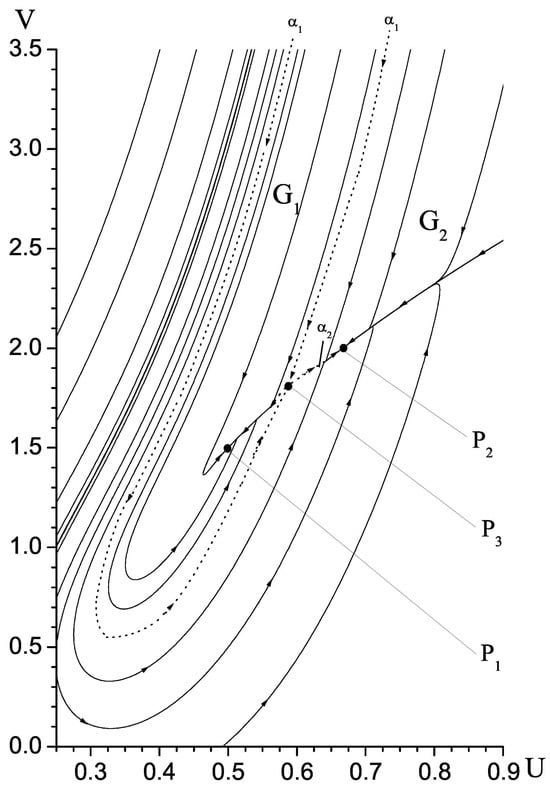
Figure 1. The first quadrant of the $(U,V)$-phase plane of solutions for the RD system (58) with ${\left(U{U}_x\right)}_x={\left(V{V}_x\right)}_x=0$.

It can be noted that the separatrix ${\alpha }_1$ (see the dotted line) divides the first quadrant into two domains, $G_1$ and $G_2$. The domain $G_1$ contains only curves leading to the stable node $P_1$, while $G_2$ contains only those leading to $P_2$. The saddle point $P_3$ is a cross-point of the separatrix ${\alpha }_1$ and the separatrix ${\alpha }_2$ (the second one is only partly pictured in Figure 1).

Now we turn to exact solutions of the RD system (58). Having the known steady-state points and using Formulas (20)–(23), we can construct four families of exact solutions in the explicit form. Thus, the stable nodes $P_1=(U_1,V_1)$ and $P_2=(U_2,V_2)$ generate the two-parameter families exact solutions

$$\begin{array}{c}U={\displaystyle \frac{1}{2}}-exp\left(-\sqrt{{\displaystyle \frac{3}{2}}}x-{\displaystyle \frac{1}{2}}t\right)\left(e_{1}sin({\displaystyle \frac{\sqrt{71}}{4}}t)+e_{2}cos({\displaystyle \frac{\sqrt{71}}{4}}t)\right)\hfill \\ V={\displaystyle \frac{3}{2}}-{\displaystyle \frac{1}{4}}exp\left(-\sqrt{{\displaystyle \frac{3}{2}}}x-{\displaystyle \frac{1}{2}}t\right)(\left(19e_1+\sqrt{71}{e}_2\right)sin({\displaystyle \frac{\sqrt{71}}{4}}t)\hfill \\ +\left(19e_2-\sqrt{71}{e}_1\right)cos({\displaystyle \frac{\sqrt{71}}{4}}t))\hfill \end{array}$$

(59)

and

$$\begin{array}{c}U={\displaystyle \frac{2}{3}}-e_{1}exp\left(-\sqrt{{\displaystyle \frac{3}{2}}}x-{\displaystyle \frac{8-\sqrt{13}}{4}}t\right)+{\displaystyle \frac{22-\sqrt{13}}{4}}{e}_{2}exp\left(-\sqrt{{\displaystyle \frac{3}{2}}}x-{\displaystyle \frac{8+\sqrt{13}}{4}}t\right)\hfill \\ V=2-{\displaystyle \frac{22-\sqrt{13}}{4}}{e}_{1}exp\left(-\sqrt{{\displaystyle \frac{3}{2}}}x-{\displaystyle \frac{8-\sqrt{13}}{4}}t\right)+27e_{2}exp\left(-\sqrt{{\displaystyle \frac{3}{2}}}x-{\displaystyle \frac{8+\sqrt{13}}{4}}t\right),\hfill \end{array}$$

(60)

for $P_1$ and $P_2$, respectively. In fact, $▵={[(a_1-a_2)+{\displaystyle \frac{3}{2}}b(V_0-U_0)]}^2+4c_1{c}_2$ is negative for $P_1$, while $▵>0$ for $P_2$; as a result, the exact solutions (59) and (60) have essential different structures. Here, $e_1$ and $e_2$ are arbitrary constants, which can be specified according to the given initial profiles.

One observes that any solution of the form (59) and (60) tends to $(U_1,V_1)$ and $(U_2,V_2)$, respectively, if $t\to +\infty$ or $x\to +\infty$. If we turn to a biological interpretation of the exact solutions obtained, then (59) and (60) may describe the prey–predator interaction with the above-mentioned asymptotic behaviour, and this means coexistence of preys and predators. Of course, both components of the exact solution must be non-negative in the domain in question. For example, the restriction $e_1^2+e_2^2\leqq 1/12$ guarantees that the exact solution (59) is non-negative in the domain $(t,x)\in (0,+\infty )\times (0,+\infty )$. The exact solution (59) with $e_1=e_2=1/5$ is plotted in Figure 2 and Figure 3.

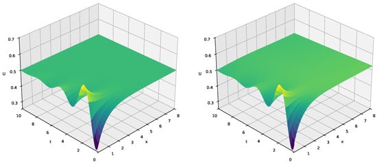
Figure 2. (Left): the component U of the exact solution (59) with $e_1=e_2=0.2$. (Right): the component U of the numerical solution obtained for the initial profile (64) with $ϵ=0.05$.

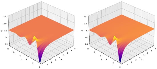
Figure 3. (Left): the component V of the exact solution (59) with $e_1=e_2=0.2$. (Right): the component V of the numerical solution obtained for the initial profile (64) with $ϵ=0.05$.

Using the properties of the exact solutions (59) and (60), one may solve some boundary-value problems. Here, we present an example in detail.

Theorem 5.

The bounded exact solution of the for the RD system (58) with the initial profiles

$$\begin{array}{c}U(0,x)={\displaystyle \frac{1}{2}}-e_{2}exp\left(-\sqrt{{\displaystyle \frac{3}{2}}}x\right)\equiv U_0\left(x\right)\hfill \\ V(0,x)={\displaystyle \frac{3}{2}}-{\displaystyle \frac{1}{4}}\left(19e_2-\sqrt{71}{e}_1\right)exp\left(-\sqrt{{\displaystyle \frac{3}{2}}}x\right)\equiv V_0\left(x\right)\hfill \end{array}$$

(61)

and the boundary conditions

$$\begin{array}{c}U(t,0)={\displaystyle \frac{1}{2}}-exp\left(-{\displaystyle \frac{1}{2}}t\right)\left(e_{1}sin({\displaystyle \frac{\sqrt{71}}{4}}t)+e_{2}cos({\displaystyle \frac{\sqrt{71}}{4}}t)\right)\hfill \\ V(t,0)={\displaystyle \frac{3}{2}}-{\displaystyle \frac{1}{4}}exp\left(-{\displaystyle \frac{1}{2}}t\right)(\left(19e_1+\sqrt{71}{e}_2\right)sin({\displaystyle \frac{\sqrt{71}}{4}}t)\hfill \\ +\left(19e_2-\sqrt{71}{e}_1\right)cos({\displaystyle \frac{\sqrt{71}}{4}}t)),\hfill \end{array}$$

(62)

and

$$U_x(t,+\infty )=0,V_x(t,+\infty )=0,$$

(63)

in the domain $(t,x)\in (0,+\infty )\times (0,+\infty )$ is given by the Formula (59).

Remark 2.

Setting either $e_2=0$, or $e_2={\displaystyle \frac{\sqrt{71}}{19}}{e}_1$, one obtains BVP with a constant initial profile for U and V, respectively. If one sets simultaneously $e_2=0$ and $e_2={\displaystyle \frac{\sqrt{71}}{19}}{e}_1$, then Formula (59) produces the steady-state solution.

Now we are looking for solutions of the above BVP with perturbed initial conditions. We are interested in knowing how these perturbations may affect the exact solution (59). Therefore, let us replace (61) by

$$U(0,x)=U_0\left(x\right)+ϵU_0\left(x\right),V(0,x)=V_0\left(x\right)+ϵV_0\left(x\right),$$

(64)

where $ϵ$ is a real parameter such that $\left|ϵ\right|<1.$

In order to construct numerical solutions of BVP (58), (62), (63), and (64), numerical simulations were conducted. These simulations utilised the odeint function from the Python scipy.integrate package (version 3.12.11), which internally employs LSODA from the FORTRAN library to solve ODEs [30]. Notably, the infinite space interval $(0,+\infty )$ was replace by the finite interval $(0,L)$ with $L=8$. Obviously, the no-flux boundary conditions at $x=8$ for exact solutions (59) and (60) are fulfilled with high exactness.

Many perturbations with different values of $ϵ$ were tested. It turns out that the value of the parameter $ϵ$ plays a crucial role on the solution behaviour and some results are presented in Figure 2, Figure 3 and Figure 4.

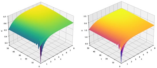
Figure 4. The numerical solution obtained for for the initial profile (64) with $ϵ=0.20$.

Figure 2 and Figure 3 represent the components U and V (right-hand-side plots) of the numerical solution, obtained for the value $ϵ=0.05$. This numerical solution has a rather similar form to the exact solution (59) pictured in Figure 2 and Figure 3 (left-hand-side plots) and practically coincides with the latter excepting a very small vicinity of $t=0$. Such a behaviour of numerical solutions has been observed for any sufficiently small $ϵ$ and even for $ϵ\simeq 0.10$.

It turns out that the situation changes drastically in the case of large perturbations of the initial conditions (61). In Figure 4, we present the components U and V of the numerical solution, obtained for the value $ϵ=0.20$. Nevertheless, the numerical solution has a similar form to the exact solution (59) for small time values, and it does not tend to (59). On the other hand, we observe that this numerical solution has the same asymptotic behaviour as the exact solution (60) excepting a vicinity of the point $x=0$. In fact, $U\to {\displaystyle \frac{2}{3}},V\to 2$ as $t\to +\infty$ for arbitrary $x\in [\delta ,+\infty ),\delta >0$. Obviously, there exists such a critical ${ϵ}_{cr}$ that any smaller $ϵ$ leads to a solution of the relevant BVP, which is sufficiently close to the exact solution (59), while any larger $ϵ$ explores a solution, which differs essentially from (59). We are going to estimate analytically and numerically ${ϵ}_{cr}$ in a forthcoming study.

The difference between the numerical solutions plotted on Figure 2, Figure 3 and Figure 4 can be explained using the $(U,V)$-phase plane of solutions (see Figure 1). In fact, the initial profile (64) with $ϵ=0.05$ produces a point belonging to the domain $G_1$. Hence, the relevant curve of the $(U,V)$-phase plane tends to the stable node $P_1$. In the case $ϵ=0.2$, one observes that the relevant point moves to the domain $G_2$, if x is sufficiently large; therefore, the solution tends to the stable node $P_2$. In the case of the sufficiently small $x>0$, the solutions of the relevant BVP still tend to the node $P_1$ because of the boundary condition (62). If this condition is replaced by the zero Neumann condition, then solutions would tend to the node $P_2$ for the arbitrary $x>0$.

Thus, the two-parameter families of exact solutions obtained in Section 2 play an important role for solving BVP (58), (62), and (63) with a wide range of initial profiles of the form (61).

Moreover, we assume that the same situation occurs for more general forms of initial profiles; however, relevant investigations lie beyond the specific aims of this study.

5. Discussion

In this work, the Lotka–Volterra type system with porous diffusion (4) was studied. The system can be considered as a simplification of the well-known SKT system (1) or as an alternative model to the classical Lotka–Volterra system with porous diffusion. Multiparameter families of exact solutions of the system in question are constructed and their properties are established. It is shown that the solutions obtained can satisfy the zero Neumann conditions, which are typical conditions for mathematical models describing real-world processes.

It should be noted that plane wave solutions can be derived as particular cases of those constructed in this work. For example, plane wave solutions of the RD system (24) can easily be derived using Formulas (20) and (23) by setting either $e_1=0$, or $e_2=0$. Interestingly, the structure of the solutions obtained is identical to that for the porous-Fisher equation presented in ([5] Section 13.4).

We also point out that the exact solutions obtained here cannot be constructed using the Lie method [31,32,33], which is extensively applied for finding exact solutions of nonlinear PDEs. In fact, using the Lie symmetry classification of the general class of RD systems with nonconstant diffusivities that was derived in [27], one easily verifies that the RD system (4) with $b_1{b}_2\ne 0$ and $c_1{c}_2\ne 0$ admits only a trivial Lie symmetry that leads to the ansatz (5).

It is proved that the system possesses two stable steady-state points provided its coefficients are correctly specified. In particular, this occurs when the system models the prey–predator interaction. A simple example of such model (see (56)) is derived that predicts two different points of coexistence of preys and predators, depending on the initial condition. It should be noted that the classical Lotka–Volterra system for the prey–predator interaction possesses only a neutrally stable centre; however, one does not possess stable steady-state nodes or spirals.

An example of the RD system with correctly specified coefficients (see system (58)), which models the prey–predator interaction, is studied in detail. The relevant exact solutions are used for solving the system with the mixed boundary conditions and initial profiles. Furthermore, a wide range of BVPs with the above boundary conditions but perturbed initial profiles are numerically solved. The exact solution is compared with numerical solutions. It is concluded that the numerical solutions coincide with the exact solution with high exactness provided perturbations of the initial profiles are sufficiently small. In the case of large perturbations of the initial profiles, the relevant numerical solutions differ essentially from the exact solution. In particular, these solutions possess different asymptotical behaviour. Thus, the exact solutions obtained play an important role for solving some boundary-value problems for the RD system (4). We note that a similar investigation for the classical Lotka–Volterra system with linear diffusion was performed in [34].

In conclusion, we point out that a similar analysis to that presented in Section 3 and Section 4 could be conducted for the RD system (4) with $b_1=b_2>0$. We expect that relevant results will be essentially different. However, a plausible biological (physical, chemical) interpretation of system (4) is needed in this case.

References

- Aris, R. The Mathematical Theory of Diffusion and Reaction in Permeable Catalysts: The Theory of the Steady State; Clarendon Press: Oxford, UK, 1975. [Google Scholar]
- Fife, P.C. Mathematical Aspects of Reacting and Diffusing Systems; Lecture Notes in Biomathematics; Springer: Berlin/Heidelberg, Germany, 1979. [Google Scholar] [CrossRef]
- Kuang, Y.; Nagy, J.D.; Eikenberry, S.E. Introduction to Mathematical Oncology, 1st ed.; CRC Press: New York, NY, USA, 2016; p. 490. [Google Scholar] [CrossRef]
- Britton, N.F. Essential Mathematical Biology; Springer Undergraduate Mathematics; Springer: Berlin/Heidelberg, Germany, 2003. [Google Scholar]
- Murray, J.D. Mathematical Biology I: An Introduction; Interdisciplinary Applied Mathematics; Springer: New York, NY, USA, 2002. [Google Scholar] [CrossRef]
- Murray, J.D. Mathematical Biology II: Spatial Models and Biomedical Applications; Interdisciplinary Applied Mathematics; Springer: New York, NY, USA, 2003. [Google Scholar] [CrossRef]
- Cherniha, R.; Davydovych, V. Nonlinear Reaction-Diffusion Systems—Conditional Symmetry, Exact Solutions and Their Applications in Biology; Lecture Notes in Mathematics; Springer: Cham, Switzerland, 2017; Volume 2196. [Google Scholar]
- Okubo, A.; Levin, S.A. Diffusion and Ecological Problems. Modern Perspectives, 2nd ed.; Interdisciplinary Applied Mathematics; Springer: Berlin/Heidelberg, Germany, 2001. [Google Scholar]
- Conway, E.D.; Smoller, J.A. Diffusion and the predator-prey interaction. SIAM J. Appl. Math. 1977, 33, 673–686. [Google Scholar] [CrossRef]
- Hastings, A. Global stability in Lotka–Volterra systems with diffusion. J. Math. Biol. 1978, 6, 163–168. [Google Scholar] [CrossRef]
- Jorné, J.; Carmi, S. Liapunov stability of the diffusive Lotka–Volterra equations. Math. Biosci. 1977, 37, 51–61. [Google Scholar] [CrossRef]
- Rothe, F. Convergence to the equilibrium state in the Volterra–Lotka diffusion equations. J. Math. Biol. 1976, 3, 319–324. [Google Scholar] [CrossRef] [PubMed]
- Cherniha, R.; Davydovych, V. Construction and application of exact solutions of the diffusive Lotka–Volterra system: A review and new results. Commun. Nonlinear Sci. Numer. Simul. 2022, 113, 106579. [Google Scholar] [CrossRef]
- Shigesada, N.; Kawasaki, K.; Teramoto, E. Spatial segregation of interacting species. J. Theor. Biol. 1979, 79, 83–99. [Google Scholar] [CrossRef]
- Pham, D.; Temam, R. A result of uniqueness of solutions of the Shigesada–Kawasaki–Teramoto equations. Adv. Nonlinear Anal. 2019, 8, 497–507. [Google Scholar] [CrossRef]
- Kan-On, Y. On the structure of positive solutions for the Shigesada–Kawasaki–Teramoto model with large interspecific competition rate. Int. J. Bifurc. Chaos 2020, 30, 2050001. [Google Scholar] [CrossRef]
- Li, Q.; Wu, Y. Existence and instability of some nontrivial steady states for the SKT competition model with large cross diffusion. Discret. Contin. Dyn. Syst. 2020, 40, 3657–3682. [Google Scholar] [CrossRef]
- Cherniha, R.; Davydovych, V.; King, J.R. The Shigesada–Kawasaki–Teramoto model: Conditional symmetries, exact solutions and their properties. Commun. Nonlinear Sci. Numer. Simul. 2023, 124, 107313. [Google Scholar] [CrossRef]
- Witelsky, T.P. Merging traveling waves for the porous-Fisher’s equation. Appl. Math. Lett. 1995, 8, 57–62. [Google Scholar] [CrossRef]
- Cherniha, R.; Dutka, V. Exact and numerical solutions of the generalized Fisher equation. Rep. Math. Phys. 2001, 47, 393–411. [Google Scholar] [CrossRef]
- Fadai, N.T.; Simpson, M.J. New travelling wave solutions of the Porous–Fisher model with a moving boundary. J. Phys. A Math. Theor. 2020, 53, 095601. [Google Scholar] [CrossRef]
- Cherniha, R. A constructive method for construction of new exact solutions of nonlinear evolution equations. Rep. Math. Phys. 1996, 38, 301–312. [Google Scholar] [CrossRef]
- Cherniha, R. New ansatze and exact solutions for nonlinear reaction-diffusion equations arising in Mathematical Biology. Symmetry Nonlinear Math. Phys. 1997, 1, 138–146. [Google Scholar]
- Cherniha, R. New Non-Lie Ansätze and Exact Solutions of Nonlinear Reaction-Diffusion-Convection Equations. J. Phys. A Math. Gen. 1998, 31, 8179–8198. [Google Scholar] [CrossRef]
- Sidorov, A.F.; Shapeev, V.P.; Yanenko, N.N. Method of Differential Relations and Its Application to Gas Dynamics; Nauka: Novosibirsk, Russia, 1984. (In Russian) [Google Scholar]
- Olver, P. Direct reduction and differential constraints. Proc. R. Soc. Lond. Ser. A Math. Phys. Sci. 1994, 46, 509–523. [Google Scholar]
- Cherniha, R.M.; King, J.R. Nonlinear reaction-diffusion systems with variable diffusivities: Lie symmetries, ansätze and exact solutions. J. Math. Anal. Appl. 2005, 308, 11–35. [Google Scholar] [CrossRef]
- Galaktionov, V.A.; Vazquez, J.L. The problem of blow-up in nonlinear parabolic equations. Discret. Contin. Dyn. Syst. 2002, 8, 399–433. [Google Scholar] [CrossRef]
- Lou, Y.; Ni, W.M. Diffusion, self-diffusion and cross-diffusion. J. Differ. Equ. 1996, 131, 79–131. [Google Scholar] [CrossRef]
- Lin, J.W.B.; Chua, S.L.T.; Bourland, J.D. Python Programming and Numerical Methods: A Guide for Engineers and Scientists; Elsevier: Amsterdam, The Netherlands, 2020. [Google Scholar]
- Bluman, G.W.; Cheviakov, A.F.; Anco, S.C. Applications of Symmetry Methods to Partial Differential Equations; Springer: New York, NY, USA, 2010. [Google Scholar]
- Arrigo, D.J. Symmetry Analysis of Differential Equations; John Wiley & Sons, Inc: Hoboken, NJ, USA, 2015. [Google Scholar]
- Cherniha, R.; Serov, M.; Pliukhin, O. Nonlinear Reaction-Diffusion-Convection Equations: Lie and Conditional Symmetry, Exact Solutions and Their Applications; Chapman & Hall/CRC Monographs and Research Notes in Mathematics, Chapman and Hall/CRC: Boca Raton, FL, USA, 2018. [Google Scholar]
- Cherniha, R.; Dutka, V. A diffusive Lotka-Volterra system: Lie symmetries, exact and numerical solutions. Ukr. Math. J. 2004, 56, 1665–1675. [Google Scholar] [CrossRef]
Disclaimer/Publisher’s Note: The statements, opinions and data contained in all publications are solely those of the individual author(s) and contributor(s) and not of MDPI and/or the editor(s). MDPI and/or the editor(s) disclaim responsibility for any injury to people or property resulting from any ideas, methods, instructions or products referred to in the content. |
© 2025 by the authors. Licensee MDPI, Basel, Switzerland. This article is an open access article distributed under the terms and conditions of the Creative Commons Attribution (CC BY) license (https://creativecommons.org/licenses/by/4.0/).