A Fractional PDE-Based Model for Nerve Impulse Transport Solved Using a Conforming Virtual Element Method: Application to Prosthetic Implants

Abstract

The main objective of this study is to present a fundamental mathematical model for nerve impulse transport, based on the underlying physical phenomena, with a straightforward application in describing the functionality of prosthetic devices. The governing equation of the resultant model is a two-dimensional nonlinear partial differential equation with a time-fractional derivative of order $\alpha \in (0,1)$. novel and effective numerical approach for solving this fractional-order problem is constructed based on the virtual element method. Three basic technical building blocks form the basis of our methodology: the regularity theory related to nonlinearity, discrete maximal regularity, and a fractional variant of the Grünwald–Letnikov approximation. By utilizing these components, along with the energy projection operator, a fully discrete virtual element scheme is formulated in such a way that it ensures stability and consistency. We establish the uniqueness and existence of the approximate solution. Numerical findings confirm the convergence in the $L^2$–norm and $H^1$–norm on both uniform square and regular Voronoi meshes, confirming the effectiveness of the proposed model and method, and their potential to support the efficient design of sensory prosthetics.

1. Introduction

Fractional calculus, the study of derivatives and integrals of non-integer orders, has increasingly become a powerful tool in modeling physical phenomena that defy conventional descriptions under ideal conditions [1]. It addresses the limitations inherent in classical models by providing a more accurate representation of systems with anomalous properties. Despite a relatively slow historical progression, the past decade has seen a renaissance, with fractional-order models advancing alongside traditional integer-order counterparts. These fractional-order models, encompassing both ordinary and partial differential equations with noninteger order terms have been instrumental in advancing our understanding of a diverse array of physical phenomena [2,3].

Over the years, notable progress has been achieved in the Finite Element Methods (FEMs) beyond the conventional finite difference schemes for fractional Equations [4,5]. For example, the work of Acosta and Borthagaray [6] clarified convergence rates for FEM approximations and regularity results for the analytical solution of the fractional Poisson problem; computational examples further support these conclusions in [7]. Ervin & Roop [8] also made contributions by using the FEM approach for steady-state fractional advection dispersion equations. Additional research explored FEM-based solutions for fractional diffusion-wave models [9], along with the Petrov–Galerkin FEM approach for fractional convection–diffusion problems in heterogeneous media [10]. Recent advances in numerical methods for fractional partial differential Equations (PDEs) have significantly improved the accuracy and stability of computational models in various applications, including impulse transport and biomedical simulations. Classical methods such as finite differences, finite elements, and spectral methods have been adapted to handle the complexities of fractional derivatives, providing valuable tools for solving these equations. In this study, we build upon existing methodologies while addressing key challenges in fractional PDE modeling. Our approach leverages the virtual element method and the Grünwald–Letnikov approximation to effectively capture the nonlocal effects inherent in fractional-order systems. Additionally, we incorporate insights from recent works, including techniques presented in [11], to further contextualize the numerical framework. We examine a few facets of time-fractional diffusion with nonlinear reactions in this work. To estimate the Riemann–Liouville-type fractional derivative, we use the first order Grünwald–Letnikov approach, which can be further extended to second-order precision. This method is chosen for its computational efficiency and ease of implementation. Furthermore, this methodology allows for an extension to second-order precision, which improves accuracy while retaining computational advantages. Unlike integral-based methods, the Grünwald–Letnikov scheme is built on discrete summation, making it particularly suitable for the computational framework adopted in this study. Higher-order accuracy in temporal directions has been attained by authors in a number of time-fractional diffusion-related model equations. For instance, the time-fractional subdiffusion Equation [12] was solved by Luo et al. using the quadratic spline collocation method. In another case, a preconditioning method for an all-at-once system from Volterra subdiffusion equations with graded time steps [13] was used for higher-order convergence in time direction, and a parallel-in-time iterative algorithm for Volterra partial integro-differential problems with weakly singular kernel was employed in [14]. Following the literature, we develop a model equation to investigate nerve impulse transport by adhering to the ideas of fractional modeling, the simultaneous physical processes, and the governing equations. Furthermore, we approximate the model equation in a fractional sense using a recently developed numerical analysis technique called the Virtual Element Method (VEM).

The VEM is a numerical method used for the solution of Partial Differential Equations (PDEs) on general polygons and polyhedrons, which in turn makes VEM a generalization of Finite Element Method (FEM) on polygonal and polyhedral meshes. Like the FEM, the VEM formulates the problem in a weak form, which involves multiplying the PDE by a test function and integrating it over the domain. The weak form allows for the use of piecewise smooth approximations and leads to a system of linear equations that can be solved numerically. Differently from FEM, the VEM introduces the concept of virtual element spaces, which are sets of functions that approximate the exact solution of the PDEs at both the local (element wise) and global level. Such functions are implicitly defined as the solution to a local PDE problem and are never explicitly constructed in the implementation of the method. The global spaces are defined on polygonal or polyhedral meshes and are constructed to be compatible with the underlying mesh structure and possess some degree of global regularity. A major advantage of the VEM is its ability to handle arbitrary polygonal and polyhedral meshes. Unlike the traditional FEM, which typically requires triangular or quadrilateral elements in 2D and tetrahedral or hexahedral elements in 3D, VEM can handle meshes composed of elements with any number of sides. This flexibility is particularly useful when dealing with complex geometries. Initially introduced to address elliptic problems such as the Poisson equation, cf. [15,16], the VEM was later applied to linear and nonlinear diffusion, convection–diffusion and convection–reaction–diffusion problems [17,18], the Stokes equations [19,20], the polyharmonic equation [21], and many other models. A recent contributed book documents the state of the art of this methodology, cf. [22]. For further reference, a detailed survey on numerical approximations of fractional models can be found in [23] and references therein.

Fractional-order models such as Huxley’s and Fischer’s equations served as inspiration for this study. Numerous physical models in different fields, such as circuit theory, population genetics, and nerve impulse transmission, are described by these equations. For further in-depth remarks on these model equations, consult the work in [24,25] and references therein. Furthermore, Zhang et al. conducted inspiring work in which they presented a local projection stabilization VEM with greater Reynold’s number for the fractional-order Burger’s Equation [26]. This study is strongly motivated in more general instances by the recent attempts at the VEM approximations of fractional-order PDEs [26,27,28]. We propose a comprehensive mathematical model for impulse transport, supported by rigorous theoretical analysis and numerical experiments. Simulations are conducted on a square domain using both uniform square and regular Voronoi meshes. The key contributions of this work are summarized below:

• Formulation of a novel mathematical model for nerve impulse transport, based on physical principles, with direct implications for the design and optimization of sensory prosthetics.
• Modeling of the governing equation as a two-dimensional nonlinear partial differential equation with a fractional time derivative ($\alpha \in (0,1)$), enhancing the realism of physiological processes.
• Development of a VEM-based numerical framework, effectively addressing challenges posed by fractional-order derivatives.
• A methodological foundation based on regularity theory for nonlinearity, discrete maximal regularity, and the fractional Grünwald–Letnikov approximation, ensuring both stability and consistency.
• Theoretical guarantees of existence and uniqueness of the approximate solution, with proofs establishing stability, a priori error bounds, and optimal convergence rates.
• Numerical validation through $L^2$-norm and $H^1$-norm convergence analysis across different mesh configurations, demonstrating the robustness of the proposed approach.
• Applicability of the model to biomedical engineering, particularly in sensory prosthetic design, reinforcing its practical significance.

These contributions position the study as a distinct and innovative effort, advancing the state of the art in fractional modeling and virtual element methods.

Paper’s outline. The structure of this paper is as follows. Section 2 outlines the physical processes and governing equations that sum up the resultant model. Section 3 presents the formulation and framework while Section 4 presents a priori bounds, and error analysis of a fully discrete virtual element method. Section 5 offers numerical examples that substantiate our theoretical findings. Section 6 concludes the paper with a summary of our work.

2. Physical Processes and Governing Equations

To develop a fundamental understanding of the behavior of the physical process at hand, we can see that there are several subprocesses that occur simultaneously. Complex phenomena modeled using fractional derivatives and integrals often exhibit nonideal behavior and anomalies. With this knowledge, we will now take each important step in the processes and create a rough model that will be utilized to investigate impulse transport through intricate geometries utilizing mathematical formulas and dependencies. In the subsection that follows, we go over each phenomenon in order to derive a consequent model.

2.1. Time-Fractional Diffusion and Reactions

It is well established that the Laplacian operator can be used to describe the simple diffusion process in the spatial domain. Specifically, for a two-dimensional Cartesian space, if u represents the physical process, the diffusion process across the domain axis $(x,y)\in {\mathbb{R}}^2$ can be described as

$$\begin{array}{cc}\hfill & {\displaystyle \frac{{\partial }^{2}u}{\partial x^2}}+{\displaystyle \frac{{\partial }^{2}u}{\partial y^2}}=0,\hfill \\ \hfill \mathrm{i}.\mathrm{e}.,& -\Delta u=0.\hfill \end{array}$$

This classical model assumes spatial homogeneity and isotropic diffusion. However, the anomalous nature of time dependence is captured using fractional derivatives, which account for memory effects in impulse transport. These considerations form the basis of our governing equation.

The temporal domain is involved in the process when it is dependent on time. It is of significant importance to highlight that the process we are modeling is not ideal; that is, the time dependency is more akin to an anomalous process than ideal/Brownian motion [29]. By incorporating a fractional time derivative into the standard diffusion equation, the process is generalized as:

$$\begin{array}{c}\hfill {\displaystyle \frac{{\partial }^{\alpha }u}{\partial t^{\alpha }}}-\Delta u=0,\end{array}$$

where $t\in (0,T)$ and $\alpha \in (0,1)$ denotes the order of the fractional derivative. While the case above assumes homogeneity, we extend the model by introducing an unknown load function $g_1$ that depends on spatial and temporal factors.

$$\begin{array}{c}\hfill {\displaystyle \frac{{\partial }^{\alpha }u}{\partial t^{\alpha }}}-\Delta u=g_1(x,y,t).\end{array}$$

(1)

This formulation reflects principles of anomalous diffusion, where transport mechanisms are nonlocal and memory-dependent. This formulation naturally extends classical diffusion equations by incorporating fractional order derivatives, providing a more realistic representation of nerve impulse transport. To provide greater clarity, we provide intermediate steps demonstrating how nonlinear terms arise from neuron interactions and impulse propagation principles. A key component of the regulating physical process is the consideration of interactions between two neurons (or nodes) in the impulse transit, defined by function u. Moreover, we define the impulse transport towards a node by $u-1$, and the impulse transport away from a node by $1-u$. This to-and-fro aspect of transport helps to explain the nonlinear nature of the response between two nodal sites. Figure 1 illustrates the characteristics of this type of response mechanism. Thus, using this knowledge, the definition of the nonlinear response term is

$$\begin{array}{c}\hfill u(u-1)(1-u)=g_2(x,y,t).\end{array}$$

(2)

where we have considered the nonhomogeneous nature of reactions for more generality. The next subsection combines these concurrent mechanisms into a unified transport model.

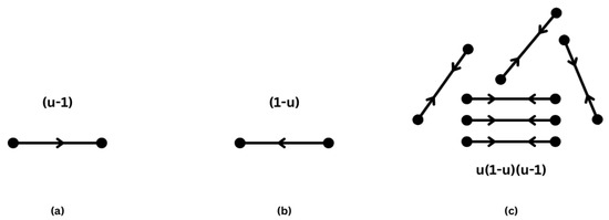
Figure 1. (a) To-natured reaction (b) fro-natured reaction, and (c) resultant reactions.

2.2. The Resultant Model

Building upon the individual governing processes discussed above, we formulate a comprehensive model by combining Equations (1) and (2):

$$\begin{array}{c}\hfill {\displaystyle \frac{{\partial }^{\alpha }u}{\partial t^{\alpha }}}-\Delta u+u(u-1)(1-u)=g_1(x,y,t)+g_2(x,y,t).\end{array}$$

The resultant model, inspired by anomalous diffusion [12], is governed by Continuous Time Random Walk (CTRW) together with the concept of Caputo-type fractional derivatives:

$$\begin{array}{c}\hfill {}^{C}D_t^{\alpha }u-\Delta u(\mathit{x},t)+f\left(u(\mathit{x},t)\right)=g(\mathit{x},t),\end{array}$$

where $\mathit{x}=(x,y)\in {\mathbb{R}}^2$ is in a polygonal domain and ${}^{C}D_t^{\alpha }u$ denotes the fractional derivative of u with respect to time in the Caputo sense [3], defined as:

$$\begin{array}{c}\hfill {}^{C}D_t^{\alpha }u\left(t\right):={\displaystyle \frac{1}{\Gamma (1-\alpha )}}{\int }_0^t{(t-s)}^{-\alpha }{\displaystyle \frac{\partial u\left(s\right)}{\partial s}}ds,\end{array}$$

where $\Gamma (·)$ denotes the Gamma function. Using these definitions, we define the complete model with initial and boundary conditions:

$$\begin{array}{c}\hfill \left\{\begin{array}{c}{}^{C}D_t^{\alpha }u-\Delta u+f\left(u\right)=g(\mathit{x},t),(\mathit{x},t)\in \Omega \times (0,T),\hfill \\ u(\mathit{x},0)=0,\mathit{x}\in \Omega ,\hfill \\ u(\mathit{x},t)=u_0,(\mathit{x},t)\in \partial \Omega \times (0,T),\hfill \end{array}\right.\end{array}$$

(3)

where $u(\mathit{x},t)$ represents the impulse response at spatial position $\mathit{x}=(x,y)$ and time t. The term ${}^{C}D_t^{\alpha }u$ incorporates memory effects of biological signal transmission. The Laplacian operator $\Delta u$ accounts for spatial diffusion, while the nonlinear function $f\left(u\right)$ models neuron interaction dynamics. The external forcing term $g(\mathit{x},t)$ represents additional stimulus sources, ensuring realistic modeling of impulse propagation in complex domains. The domain $\Omega$ is a bounded polygonal region in ${\mathbb{R}}^2$. Boundary conditions are designed to reflect the physical properties of nerve impulse transmission, supporting numerical stability and realistic modeling. The initial condition,

$$\begin{array}{c}\hfill u(\mathit{x},0)=0,\mathit{x}\in \Omega \end{array}$$

indicates that at $t=0$, no impulse has been transmitted, representing an inactive neuronal state before stimulation. The boundary condition,

$$\begin{array}{c}\hfill u(\mathit{x},t)=u_0,(\mathit{x},t)\in \partial \Omega \times (0,T)\end{array}$$

ensures a prescribed impulse response at the domain boundary, which could correspond to sustained stimulation or fixed neuronal activity levels. Depending on the physical constraints, different boundary types may be appropriate: Dirichlet conditions enforce fixed impulse values, Neumann conditions regulate impulse flux, and Robin conditions provide a weighted combination of both. These boundary formulations contribute to an accurate representation of real-world neuronal behavior. Dirichlet conditions ensure a controlled and predefined stimulation at the boundary, which is relevant for prosthetic applications; we also acknowledge that alternative boundary formulations, such as Neumann or Robin conditions, may better capture certain physiological behaviors.

As a result, (3) defines our impulse transport model. In the next section, we will present the discretized framework, formulation, and fundamental VEM concepts.

3. The Virtual Element Method

We consider the fractional-order nonlinear PDE model given in (3). The domain $\Omega$ is partitioned into a shape-regular polygonal mesh ${\mathcal{T}}_h$, with $h_E$ the diameter of an element $E\in {\mathcal{T}}_h$. Also, let

$$\begin{array}{c}\hfill h:=\underset{E\in {\mathcal{T}}_h}{\max }{h}_E.\end{array}$$

For mesh regularity, there exists $\rho >0$, so for every $E\in {\mathcal{T}}_h$, we assume the following:

• For a ball with radius $\ge \rho h_E$, E has a star shape;
• The distance between any two of its vertices is $\ge \rho h_E$.

Referring to [16], for $k\ge \mathbb{N}$, the local virtual element space $V_h^E$ of order k is defined as,

$$\begin{array}{c}\hfill V_h^E=\left\{v_h\in H^1\left(E\right):\Delta v_h\in {\mathbb{P}}_k\left(E\right),v_h{{|}_{\partial E}\in C^0(\partial E),v_h|}_e\in {\mathbb{P}}_k\left(e\right)\forall e\subset \partial E\right\},\end{array}$$

where $\partial E$ is the polygonal boundary of E and $e\subset \partial E$ denotes a generic edge.

Next, we define some useful polynomial projection operators. We consider the elliptic projection operator ${\Pi }_k^{\nabla ,E}:H_0^1\left(E\right)\to {\mathbb{P}}_k\left(E\right)$, which is the orthogonal projector onto the space of polynomials of degree k with respect to the $H^1$ semi-norm. Formally, for every $v\in H_0^1\left(E\right)$, the k-degree polynomial ${\Pi }_k^{\nabla ,E}v$ is the solution to the variational problem

$$\begin{array}{cc}\hfill \underset{E}{\int }\nabla \left({\Pi }_k^{\nabla ,E}v-v\right)·\nabla q_{k}dx& =0,\forall q_k\in {\mathbb{P}}_k\left(E\right),\hfill \\ \hfill \underset{\partial E}{\int }\left({\Pi }_k^{\nabla ,E}v-v\right)ds& =0,\hfill \end{array}$$

where the second condition is needed to fix the gradient kernel. We also define the $L^2$-orthogonal projection operator ${\Pi }_k^{0,E}:H_0^1\left(E\right)\to {\mathbb{P}}_k\left(E\right)$, such that for any $v\in H_0^1\left(E\right)$, the polynomial ${\Pi }_k^{0,E}v$ satisfies:

$$\begin{array}{cc}\hfill \underset{E}{\int }\left({\Pi }_k^{0,E}v-v\right)q_{k}dx& =0,\forall q_k\in {\mathbb{P}}_k\left(E\right).\hfill \end{array}$$

For each $E\in {\mathcal{T}}_h$, we define the locally “enhanced" virtual element space by utilizing the elliptic projection operator as

$$\begin{array}{c}\hfill W_h^E=\{w_h\in V_h^E:\underset{E}{\int }\left({\Pi }_{E,k}^{\nabla }{w}_h\right)q_{k}dx=\underset{E}{\int }{w}_h{q}_{k}dx,\forall q_k\in {\mathbb{P}}_k/{\mathbb{P}}_{k-2}\left(E\right)\},\end{array}$$

where two polynomials are considered equivalent if the degree of their difference does not exceed $k-2$. This equivalence plays a crucial role in defining the virtual element spaces. Specifically, the union of the spaces of homogeneous polynomials of exact degrees k and $k-1$ serves as a key component in the implementation. This structure ensures that the polynomial basis captures the necessary degrees of freedom and maintains consistency within the approximation framework. For polynomial equivalence classes, the quotient space is represented by ${\mathbb{P}}_k/{\mathbb{P}}_{k-2}\left(E\right)$. By assembling the local VEM spaces, the global VEM space is produced and is given as

$$\begin{array}{c}\hfill W_h=\{w\in H_0^1(\Omega ):w{|}_E\in W_h^E,\forall E\in {\mathcal{T}}_h\},\end{array}$$

where ${\mathcal{T}}_h$ is a shape-regularized polygonization of $\Omega$.

Any virtual element function in $w_h\in W_h^E$ is specifically characterized as follows, which we can interpret as the fundamental Degrees of Freedoms (DoFs) displayed in Figure 2 and Figure 3:

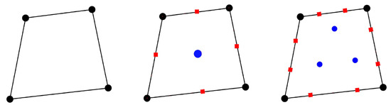
Figure 2. Boundary and internal degrees of freedom for conforming VEM of order k = 1, 2, and 3, respectively, where black circles on vertices represent (D1), red squares on edges represent (D2), and blue circles represent (D3).

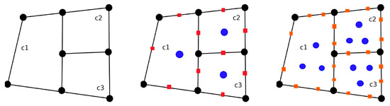
Figure 3. Element-wise boundary and internal degrees of freedom for conforming VEM of order k = 1, 2, and 3, respectively, where black circles on vertices represent (D1), orange squares on edges represent (D2), and blue circles represent (D3).

(D1) 

The vertex values $w_h\left(V_i\right)$ for $k\ge 1$, where the vertices of an element E for $k\ge 1$ are denoted by $V_i$;

(D2) 

On each edge e of $\partial E$ for $k>1$, the values of $w_h$ at the $(k-1)$ internal Gauss–Lobatto quadrature points;

(D3) 

The polynomial moments for $k\ge 2$:

$$\begin{array}{c}\hfill \underset{E}{\int }{v}_h{p}_{k-2}dx,\forall p_{k-2}\in {\mathbb{P}}_{k-2}\left(E\right).\end{array}$$

The local DoFs of the spaces $W_h^E$ from all the elements $E\in {\mathcal{T}}_h$ are collected in a $H^1$-conforming manner to yield the DoFs of the global virtual element space of order k. The unisolvence of these degrees of freedom is proved in [16]. The projections ${\Pi }_k^{\nabla ,E}{w}_h$ and ${\Pi }_k^{0,E}{w}_h$ are computable from the degrees of freedom (D1)–(D3) of $w_h\in W_h^E$, which is a fundamental characteristic of the concept of local VEM space.

3.1. Virtual Element Discretization

To discretize the developed model Equation (3), we follow the stated principles of VEM. For the time-fractional derivative, we devise a discrete form with the help of Grünwald–Letnikov approximation. The authors in [24] devised a discrete fractional Grönwall-type inequality for the Caputo-type fractional derivative. We provide a discrete fractional Grönwall-type inequality (Grünwald–Letnikov approximation) to the fractional Riemann–Liouville-type derivative, motivated by this work. We utilize the relationship between Caputo and Riemann–Liouville (R-L)-type derivatives, which is represented as

$$\begin{array}{c}\hfill {}^{C}D_t^{\alpha }u\left(t\right)={}^{R}D_t^{\alpha }(u\left(t\right)-u\left(0\right)).\end{array}$$

Considering $u(x,0)=0$, we employ the equivalence ${}^{C}D_t^{\alpha }u\left(t\right)={}^{R}D_t^{\alpha }u\left(t\right)$, where ${}^{R}D_t^{\alpha }$ represents the Riemann–Liouville derivative of order $\alpha$.

As a result, the governing equation can be reformulated using the Riemann–Liouville fractional derivative as follows:

$$\begin{array}{c}\hfill \left\{\begin{array}{c}{}^{R}D_t^{\alpha }u-\Delta u+f\left(u(\mathit{x},t)\right)=g(\mathit{x},t),(\mathit{x},t)\in \Omega \times (0,T),\hfill \\ u(\mathit{x},0)=0,\mathit{x}\in \Omega ,\hfill \\ u(\mathit{x},t)=0,(\mathit{x},t)\in \partial \Omega \times (0,T).\hfill \end{array}\right.\end{array}$$

where $\mathit{x}\in \Omega$ denotes the spatial domain, u represents the dependent variable, $f\left(u\right)$ is the nonlinear term, and $g(\mathit{x},t)$ is the external forcing function.

The weak/variational formulation of this model equation is as follows:

Find $u\left(t\right)\in H_0^1(\Omega )$ for almost all $t\in (0,T]$ such that

$$\begin{array}{c}\hfill \left\{\begin{array}{cc}m{(}^R{D}_t^{\alpha }u,w)+a(u,w)+⟨f\left(u\right),w⟩=⟨g,w⟩\hfill & \forall w\in H_0^1(\Omega ),t\in (0,T),\hfill \\ u(\mathit{x},0)=0,\hfill & \mathit{x}\in \Omega ,\hfill \end{array}\right.\end{array}$$

(4)

where the bilinear forms $m(·,·)$ and $a(·,·)$ are defined as:

$$\begin{array}{c}\hfill m(w,v)=\underset{\Omega }{\int }wvdx,a(w,v)=\underset{\Omega }{\int }\nabla w·\nabla vs.dx\forall w,v\in H_0^1(\Omega ),\end{array}$$

and $⟨·,·⟩$ is the duality product in $L^2(\Omega )$. The well-posedness results of the weak form are proved in the work of Jin et al. [10,30] for time-fractional nonlinear subdiffusion equations.

The semi-discrete VEM scheme corresponding to the given problem is as follows:

Find $u_h(\mathit{x},t)\in W_h$, such that,

$$\begin{array}{c}\hfill \left\{\begin{array}{c}{m}_h({}^{R}D_t^{\alpha }{u}_h,w_h)+a_h(u_h,w_h)+⟨f_h\left(u_h\left(t\right)\right),w_h⟩=⟨g_h,w_h⟩\forall w_h\in W_h\hfill \\ u_h(\mathit{x},0)=0,\mathit{x}\in \Omega .\hfill \end{array}\right.\end{array}$$

where the discrete global bilinear forms $a_h(·,·):W_h\times W_h\to \mathbb{R}\mathrm{and}{m}_h(·,·):W_h\times W_h\to \mathbb{R}$ are defined as:

$$\begin{array}{cc}\hfill & a_h(v,v)=\sum _{E\in {\mathcal{T}}_h}{a}_h^E(v,v)\forall vs.\in W_h,\hfill \\ \hfill & m_h(v,v)=\sum _{E\in {\mathcal{T}}_h}{m}_h^E(v,v)\forall vs.\in W_h,\hfill \end{array}$$

where both $a_h^E(·,·):W_h^E\times W_h^E\to \mathbb{R}\mathrm{and}{m}_h^E(·,·):W_h^E\times W_h^E\to \mathbb{R}$ are locally computable bilinear forms defined as follows:

$$\begin{array}{c}\hfill a_h^E(v_h,w_h)=a^E({\Pi }_k^{\nabla ,E}{u}_h,{\Pi }_k^{\nabla ,E}{v}_h)+s_a^E((I-{\Pi }_k^{\nabla ,E})u_h,(I-{\Pi }_k^{\nabla ,E})v_h)\forall u_h,v_h\in W_h^E,\\ \hfill m_h^E(v_h,w_h)=m^E({\Pi }_k^{0,E}{u}_h,{\Pi }_k^{0,E}{v}_h)+s_m^E((I-{\Pi }_k^{0,E})u_h,(I-{\Pi }_k^{0,E})v_h)\forall u_h,v_h\in W_h^E,\end{array}$$

where the bilinear forms $s_a^E:W_h^E\times W_h^E\to \mathbb{R}$ and $s_m^E:W_h^E\times W_h^E\to \mathbb{R}$ are locally admissible stabilizing terms that are symmetric positive definite and satisfy

$$\begin{array}{c}\hfill c_0{a}^E(v_h,v_h)\le s_a^E(v_h,v_h)\le c_1{a}^E(v_h,v_h)\forall v_h\in W_h^E,\\ \hfill d_0{m}^E(v_h,v_h)\le s_m^E(v_h,v_h)\le d_1{m}^E(v_h,v_h)\forall v_h\in W_h^E,\end{array}$$

for some positive constants $c_0,c_1,d_0\mathrm{and}{d}_1$ independent of h and E.

The stability of local bilinear forms $a_h^E(·,·)$ and $m_h^E(·,·)$ is guaranteed by these stabilization terms (a formal description is given below). This work adopts the $computable$ “dofi-dofi” stabilization (see [31]) and these are essential components of the VEM, to ensure numerical stability and consistency on general polygonal meshes. We provide explicit definitions of the stabilization terms $s_a^E$ and $s_m^E$ as follows:

• Stabilization for Stiffness Term:

The stiffness stabilization term $s_a^E(u,v)$ is defined as:

$$s_a^E(u,v)=\sum _{i,j=1}^{N_E}{\mathrm{dof}}_i\left(u\right){\mathrm{dof}}_j\left(v\right),$$

where $N_E$ is the number of degrees of freedom for the element and ${\mathrm{dof}}_i\left(u\right)$ and ${\mathrm{dof}}_j\left(v\right)$ represent the values of the solution and test functions at the respective degrees of freedom.

• Stabilization for Mass Term:

The mass stabilization term $s_m^E(u,v)$ is defined as:

$$s_m^E(u,v)=h_E^2\sum _{i,j=1}^{N_E}{\mathrm{dof}}_i\left(u\right){\mathrm{dof}}_j\left(v\right),$$

where $h_E$ is the diameter of the element E, $N_E$ is the number of degrees of freedom, and ${\mathrm{dof}}_i\left(u\right)$, ${\mathrm{dof}}_j\left(v\right)$ correspond to the values of the solution and test functions at the respective degrees of freedom.

We recall that the bilinear forms $a_h^E(·,·)$ and $m_h^E(·,·)$ possess the fundamental properties of

Consistency: $\forall E\in {\mathcal{T}}_h$ and for any $w_h\in W_h^E$, it holds that

$$\begin{array}{cc}\hfill a_h^E(p,w_h)& =a^E(p,w_h)\forall p\in {\mathbb{P}}_k\left(E\right),\hfill \\ \hfill m_h^E(p,w_h)& =m^E(p,w_h)\forall p\in {\mathbb{P}}_k\left(E\right).\hfill \end{array}$$

Stability: Two constant pairs that are independent of h exist, say, $({\alpha }_{*},{\alpha }^{*})$ and $({\gamma }_{*},{\gamma }^{*})$ with $0<{\alpha }_{*}\le {\alpha }^{*}$ and $0<{\gamma }_{*}\le {\gamma }^{*}$, such that for all $w_h\in W_h^E$, the two following equivalence holds:

$$\begin{array}{cc}\hfill & {\alpha }_{*}{a}^E(w_h,w_h)\le a_h^E(w_h,w_h)\le {\alpha }^{*}{a}^E(w_h,w_h),\hfill \\ \hfill & {\gamma }_{*}{m}^E(w_h,w_h)\le m_h^E(w_h,w_h)\le {\gamma }^{*}{m}^E(w_h,w_h).\hfill \end{array}$$

The conditions above ensure that the non-polynomial parts $s_a^E(·,·)$ and $s_m^E(·,·)$ scale the same as the polynomial parts of $a_h^E(·,·)$ and $m_h^E(·,·)$, respectively.

To compute the nonlinear forcing term, we use the $L^2$-orthogonal projector ${\Pi }_k^{0,E}$ previously defined. For each element E, we first define $f_h\left(u_h\right)$ as

$$\begin{array}{c}\hfill f_h\left(u_h\right){|}_E:={\Pi }_k^{0,E}\left(f\left({\Pi }_k^{0,E}{u}_h\right)\right)\mathrm{on}\mathrm{each}E\in {\mathcal{T}}_h.\end{array}$$

The orthogonality of ${\Pi }_k^{0,E}$ implies that

$$\begin{array}{c}\hfill ⟨f_h\left(u_h\right),v_h⟩=\sum _{E\in {\mathcal{T}}_h}\underset{E}{\int }{f}_h\left(u_h\right)v_{h}dx=\sum _{E\in {\mathcal{T}}_h}\underset{E}{\int }{\Pi }_k^{0,E}\left(f\left({\Pi }_k^{0,E}{u}_h\right)\right)v_{h}dx=\sum _{E\in {\mathcal{T}}_h}\underset{E}{\int }f\left({\Pi }_k^{0,E}{u}_h\right){\Pi }_k^{0,E}{v}_{h}dx.\end{array}$$

Hence, for $f\left(u_h\right)\in L^2(\Omega )$ and $u_h\in W_h$, we state that

$$\begin{array}{c}\hfill f_h\left(u_h\right):={\Pi }_k^0\left(f\left({\Pi }_k^0{u}_h\right)\right),\end{array}$$

by introducing a global $L^2$-orthogonal projection operator ${\Pi }_k^0:L^2(\Omega )\to {\mathbb{P}}_k\left({\mathcal{T}}_h\right)$ onto the piecewise polynomial space of degree k built on the mesh partition ${\mathcal{T}}_h$. The global projection operator is such that

$$\begin{array}{c}\hfill {\Pi }_k^0\left(f\left({\Pi }_k^0{u}_h\right)\right){|}_E={\Pi }_k^{0,E}\left(f\left({\Pi }_k^{0,E}{u}_h\right)\right)\forall E\in {\mathcal{T}}_h.\end{array}$$

We outlined that this approximation of the forcing term is computable since the projection ${\Pi }_k^{0,E}{u}_h$ is computable from the degrees of freedom of $u_h$ in the enhanced space $W_h^E$.

3.2. Fully Discrete VEM

The Grünwald–Letnikov approximation and the Caputo definition provide comprehensive approaches to approximate fractional derivatives with first-order and second-order accuracy, respectively. These methodologies enable a finite-sum representation of fractional derivatives involving integer-order derivatives, facilitating their computation. To construct a fully discrete scheme, it is necessary to evaluate the fractional derivative along the temporal axis. Consider a uniform partitioning of the interval $(0,T]$ into K subintervals, where $t_0<t_1<···<t_K$ and the step size is $\tau$. By applying the Grünwald–Letnikov approximation to the Riemann–Liouville-type derivative [32], the fractional derivative can be computed as:

$$\begin{array}{c}\hfill {}^{R}D_{t_n}^{\alpha }\psi (·,t)={\tau }^{-\alpha }\sum _{i=0}^n{w}_{n-i}^{\left(\alpha \right)}\psi (·,t_i)+{\mathit{R}}_{\mathit{n}},\end{array}$$

(5)

where $w_i^{\left(\alpha \right)}$ represents the fractional weights associated with the approximation. The weights are calculated in this case using

$$\begin{array}{c}\hfill w_i^{\left(\alpha \right)}={(-1)}^i{\displaystyle \frac{\Gamma (\alpha +1)}{\Gamma (i+1)\Gamma (\alpha -i+1)}},\end{array}$$

and the error ${\mathit{R}}_{\mathit{n}}$ satisfies the estimate, $\left|\right|{\mathit{R}}_{\mathit{n}}\left|\right|\le c\tau$ [1].

Remark 1.

In order to achieve an accuracy of $\mathcal{O}\left({\tau }^2\right)$, Jin et al. [33] utilized the following approximation to the R-L-type derivative at the point $t=t_{n-{\displaystyle \frac{\alpha }{2}}}$ as:

$$\begin{array}{c}\hfill {}^{R}D_t^{\alpha }\varphi (\mathit{x},t_n)={{}^{R}D_t^{\alpha }}_{n-\frac{\alpha }{2}}\varphi (\mathit{x},t)+\mathcal{O}\left({\tau }^2\right),\end{array}$$

where ${}^{R}D_t^{\alpha }$ is a discrete fractional differential operator defined as

$$\begin{array}{c}\hfill {}^{R}D_t^{\alpha }\varphi (\mathit{x},t_n):={\tau }^{-\alpha }\sum _{i=0}^n{w}_{n-i}^{\left(\alpha \right)}\varphi (\mathit{x},t_i).\end{array}$$

(6)

Under specific compatibility conditions and the regularity assumption $\varphi \in C^3[0,T]$, Dimitrov [34] made the initial observation of this accuracy.

Denote $U_h^{n,\theta }=\left(1-{\displaystyle \frac{\theta }{2}}\right)U_h^n+{\displaystyle \frac{\theta }{2}}{U}_h^{n-1}$, where $0\le \theta \le 1$. For any arbitrary choice of $\theta \in [0,1]$ in the discrete scheme, the numerical results show no significant effect on the accuracy, regardless of the fractional-order $\alpha \in (0,1)$. Hence, for the sake of convenience and to reduce notational complexity, we fix $\theta =\alpha$ in the following fully discrete VEM formulation:

Determine $U_h^n\in W_h$, for $n=1,2,\dots ,K$, such that:

$$\begin{array}{c}\hfill \left\{\begin{array}{c}{m}_h({}^{R}D_t^{\alpha }{U}_h^n,v_h)+a_h(U_h^{n,\alpha },v_h)+⟨f\left(U_h^{n,\alpha }\right),v_h⟩=⟨g_h,v_h⟩\forall v_h\in W_h,\hfill \\ U_h^0=0.\hfill \end{array}\right.\end{array}$$

By applying the definition of the discrete fractional operator ${}^{R}D_t^{\alpha }$ given in (6), the equation is reformulated as:

$$\begin{array}{c}\hfill {\tau }^{-\alpha }{w}_0^{\left(\alpha \right)}{m}_h(U_h^n,v_h)+a_h(U_h^{n,\alpha },v_h)+⟨f\left(U_h^{n,\alpha }\right),v_h⟩=⟨g_h,v_h⟩-{\tau }^{-\alpha }\sum _{j=1}^{n-1}{w}_{n-j}^{\left(\alpha \right)}{m}_h(U_h^j,v_h).\end{array}$$

(7)

This discrete reformulation results in a system of K algebraic equations that is $\mathcal{O}\left(\tau \right)$ accurate in time and can be efficiently solved to obtain the virtual element approximation of the solution.

3.3. VEM Implementation

Let $\beta$ be the dimension, and let ${\left\{{\varphi }_j\right\}}_{j=1}^{\beta }$ be the canonical basis of the global virtual element space $W_h$. Consider $U_h^n\in W_h$ with its associated DoF vector ${\nu }^{\left(n\right)}:={({\nu }_1^n,{\nu }_2^n,\dots ,{\nu }_{\beta }^n)}^T$, where ${\nu }_i^n$ is the $i^{th}$ DoF of $U_h^n$. Then, we have the expression

$$U_h^n=\sum _{\ell =1}^{\beta }{\nu }_{\ell }^n{\varphi }_{\ell }.$$

(8)

Substituting this expansion into the definition of the operator ${}^{R}D_{t_n}^{\alpha }$ from Equation (2) and taking $v_h={\varphi }_i$ in the discrete scheme (7), we obtain the following system of equations for $i=1,\dots ,\beta$

$$\begin{array}{ccc}& & {\tau }^{-\alpha }{w}_0^{\left(\alpha \right)}{m}_h\left(\sum _{\ell =1}^{\beta }{\nu }_{\ell }^n{\varphi }_{\ell },{\varphi }_i\right)+\left(1-{\displaystyle \frac{\alpha }{2}}\right)a_h\left(\sum _{\ell =1}^{\beta }{\nu }_{\ell }^n{\varphi }_{\ell },{\varphi }_i\right)+\left(1-{\displaystyle \frac{\alpha }{2}}\right)⟨\sum _{\ell =1}^{\beta }{\nu }_{\ell }^n{\varphi }_{\ell },{\varphi }_i⟩=\hfill \\ & & \left(1-{\displaystyle \frac{\alpha }{2}}\right)⟨g_h^n,{\varphi }_i⟩+{\displaystyle \frac{\alpha }{2}}⟨g_h^{n-1},{\varphi }_i⟩-{\displaystyle \frac{\alpha }{2}}{a}_h\left(\sum _{\ell =1}^{\beta }{\nu }_{\ell }^{n-1}{\varphi }_{\ell },{\varphi }_i\right)-{\displaystyle \frac{\alpha }{2}}⟨\sum _{\ell =1}^{\beta }{\nu }_{\ell }^{n-1}{\varphi }_{\ell },{\varphi }_i⟩\hfill \\ & & -{\tau }^{-\alpha }\sum _{j=1}^{n-1}{w}_{n-j}^{\left(\alpha \right)}{m}_h\left(\sum _{\ell =1}^{\beta }{\nu }_{\ell }^j{\varphi }_{\ell },{\varphi }_i\right).\hfill \end{array}$$

Let us denote M $={\left(m_h({\varphi }_{\ell },{\varphi }_i)\right)}_{\ell ,i=1}^{\beta }$, A $={\left(a_h({\varphi }_{\ell },{\varphi }_i)\right)}_{\ell ,i=1}^{\beta }$, and C $={⟨f_h\left({\varphi }_{\ell }\right),{\varphi }_i)⟩}_{\ell ,i=1}^{\beta }$, which represent the global matrix forms of the bilinear forms $m_h(·,·)$, $a_h(·,·)$, $b_h(·,·)$, and the scalar product $<·,·>$, respectively. A load vector (column) at time step n is denoted as ${\mathbf{S}}^{\left(n\right)}={\left(⟨g_h^n,{\varphi }_i⟩\right)}_{i=1}^{\beta }$. Using these notations, the above system can be conveniently expressed in matrix form as,

$$\begin{array}{cc}\hfill \left(w_0^{\left(\alpha \right)}\mathbf{M}+{\tau }^{\alpha }\left(1-{\displaystyle \frac{\alpha }{2}}\right)(\mathbf{A}+\mathbf{C})\right){\nu }^{\left(n\right)}& ={\tau }^{\alpha }\left\{\left(1-{\displaystyle \frac{\alpha }{2}}\right){\mathbf{S}}^{\left(n\right)}+{\displaystyle \frac{\alpha }{2}}{\mathbf{S}}^{(n-1)}-{\displaystyle \frac{\alpha }{2}}(\mathbf{A}+\mathbf{C}){\nu }^{(n-1)}\right\}\hfill \\ \hfill & -\sum _{j=1}^{n-1}{w}_{n-j}^{\left(\alpha \right)}\mathbf{M}{\nu }^{\left(j\right)}.\hfill \end{array}$$

(9)

Any effective iterative technique can be used to solve the above nonlinear algebraic system. In this work, we use Newton’s method to solve the resulting system at each time step. It is important to note that in the discrete formulation, the numerical solution at nth time step depends on the solutions that were computed at all preceding time steps, 1, 2, ..., $n-1$. The following specifications were used for the implementation of Newton’s method:

3.3.1. Hardware Specifications

• Device: HP Z2 Tower G9 Workstation Desktop PC.
• Processor: 13th Gen Intel(R) Core(TM) i7-13700K 3.40 GHz for efficient computations.
• Memory: 128 GB RAM.
• Storage: Solid State Drive (SSD) for faster data access and execution (1.86 TB).

3.3.2. Software and Implementation

• Software: MATLAB (Version R2021a).
• Key MATLAB Toolboxes: Symbolic Math Toolbox, Optimization Toolbox, Parallel Computing Toolbox.
• Numerical Method: Newton’s method is used to iteratively solve the nonlinear system, leveraging automatic differentiation via the Jacobian function.
• Convergence Criteria: The iterative solver stops when $\parallel F\left(x\right)\parallel <ϵ$, where $ϵ$ is a predefined tolerance level.

4. Theoretical Analysis and a Priori Error Estimates

Throughout this section, we introduce the notations used in our theoretical analysis. Let $\Omega$ be a domain, and let $v\in L^2(\Omega )$ denote an arbitrary function. The $L^2$ inner product is given by:

$$⟨v,w⟩=\underset{\Omega }{\int }v\left(x\right)w\left(x\right)dx,$$

and the associated $L^2(\Omega )$ norm is defined as:

$$\parallel v\parallel ={\left(\underset{\Omega }{\int }v\left(x\right)v\left(x\right)dx\right)}^{1/2}.$$

For a nonnegative integer n, the Sobolev space $H^n(\Omega )$ is equipped with the norm:

$${\parallel w\parallel }_n={\left(\sum _{0\le s\le n}{∥{\displaystyle \frac{{\partial }^{s}w}{\partial x^s}}∥}^2\right)}^{1/2}.$$

The space $C_0^{\infty }(\Omega )$ denotes the set of infinitely differentiable functions with compact support in $\Omega$. Its closure with respect to the norm ${\parallel ·\parallel }_m$ is denoted by $H_0^m(\Omega )$. Finally, ${\mathbb{P}}_k(\Omega )$ represents the set of all polynomials over $\Omega$ with degree at most k.

We note that in numerical analysis, first-order accuracy refers to methods where the error term is proportional to the first power of the discretized step size, meaning that the error decreases linearly as the step size is reduced. Second-order accuracy indicates that the error term scales quadratically with the step size, offering improved precision compared to first-order methods. Second-order precision specifically pertains to numerical approximation techniques that achieve second-order accuracy in estimating derivatives or solving equations. In the context of fractional calculus, employing higher-order precision enhances the accuracy of numerical schemes while preserving computational efficiency. Throughout this work, we utilize the Grünwald–Letnikov approximation ensuring a reliable representation of fractional derivatives.

To establish the existence and uniqueness of the solution to the model problem (1), we impose the following assumptions on f and g:

Hypothesis 1.

The function $f:\mathbb{R}\to \mathbb{R}$, satisfies the Lipschitz condition:

$$|f\left(v_1\right)-f\left(v_2\right)|\le \mathcal{L}|v_1-v_2|,$$

for $v_1,v_2\in \mathbb{R}$ and some $\mathcal{L}>0$.

Hypothesis 2.

The load term $g(\mathit{x},t)$ belongs to the $L^2$-space, implying that

$${\parallel g(x,t)\parallel }_{L^2(\Omega )}={\left(\underset{\Omega }{\int }{\left|g(x,t)\right|}^{2}dx\right)}^{1/2}\le C_g,$$

where $C_g$ is a positive constant independent of x and t.

The existence and uniqueness of the solution to problem (1) are established by the following well-posed theorem, the proof of which can be found in [24,30].

Theorem 1.

Under the assumption  (H1), Equation (1) admits a unique solution ψ for $\alpha \in (0,1)$, satisfying:

$$\begin{array}{cc}\hfill & \left(i\right)\psi \in C^{\alpha }([0,T];L^2(\Omega ))\cap C([0,T];H_0^1(\Omega )\cap H^2(\Omega )),\hfill \\ \hfill & \left(ii\right){}^{C}D_t^{\alpha }\psi \in C([0,T];L^2(\Omega )),{\displaystyle \frac{\partial \psi \left(t\right)}{\partial t}}\in L^2(\Omega ),\hfill \\ \hfill & \left(iii\right)\parallel {\displaystyle \frac{\partial \psi \left(t\right)}{\partial t}}\parallel \le C{t}^{\alpha -1},\mathit{for}t\in (0,T],\hfill \end{array}$$

where $C>0$ is a constant independent of ψ.

To establish the convergence of the VEM, we derive appropriate a priori error bounds. The fractional Grünwald-type inequality plays a critical role in this analysis.

The Grünwald weights $w_i^{\left(\alpha \right)}$ can be computed recursively as follows:

$$\begin{array}{c}\hfill w_0^{\left(\alpha \right)}=1,w_i^{\left(\alpha \right)}=\left(1-{\displaystyle \frac{\alpha +1}{i}}\right)w_{i-1}^{\left(\alpha \right)},\mathrm{for}i\ge 1.\end{array}$$

Additionally, define the cumulative weights $g_n^{\left(\alpha \right)}={\sum }_{i=1}^n{w}_i^{\left(\alpha \right)}$. Then, we have:

$$\begin{array}{c}\hfill g_0^{\left(\alpha \right)}=w_0^{\left(\alpha \right)},w_i^{\left(\alpha \right)}=g_i^{\left(\alpha \right)}-g_{i-1}^{\left(\alpha \right)},i\in [1,n].\end{array}$$

The weights $w_i^{\left(\alpha \right)}$ satisfy the following properties:

$$\begin{array}{c}\hfill w_0^{\left(\alpha \right)}=1,-1<w_1^{\left(\alpha \right)}<w_2^{\left(\alpha \right)}<\dots <w_i^{\left(\alpha \right)}<\dots <0,\sum _{i=0}^{\infty }{w}_i^{\left(\alpha \right)}=0.\end{array}$$

(10)

Consequently, $g_{i-1}^{\left(\alpha \right)}>g_i^{\left(\alpha \right)}$ for $i=1,\dots ,n$. Using these weights, we can reformulate the Riemann–Liouville fractional derivative as:

$$\begin{array}{c}\hfill {}^{R}D_t^{\alpha }u(·,t_n)={\tau }^{-\alpha }\sum _{i=1}^n\left(g_i^{\left(\alpha \right)}-g_{i-1}^{\left(\alpha \right)}\right)u(·,t_{n-i})+{\tau }^{-\alpha }{g}_0^{\left(\alpha \right)}u(·,t_n).\end{array}$$

(11)

Using the initial condition $u(·,t_0)=0$, this simplifies to:

$$\begin{array}{c}\hfill {}^{R}D_t^{\alpha }u(·,t_n)={\tau }^{-\alpha }\sum _{i=1}^n{g}_{n-i}^{\left(\alpha \right)}\delta u(·,t_i),\end{array}$$

where $\delta u(·,t_i)=u(·,t_i)-u(·,t_{i-1})$ for $i=1,\dots ,n$.

To prove existence and uniqueness of the solution to the fully discrete VEM, we apply a proposition based on Brouwer’s Fixed Point Theorem [35]:

Proposition 1.

Let $\mathcal{H}$ be a finite-dimensional Hilbert space with norm $\left|\right|·\left|\right|$ and inner product $⟨·,·⟩$. Let $G:\mathcal{H}\to \mathcal{H}$ be a continuous map such that,

$$\begin{array}{c}\hfill ⟨G\left(w\right),w⟩>0\mathrm{for}\mathrm{all}w\in \mathcal{H}\mathrm{with}\left|\right|w\left|\right|=\rho ,\rho >0,\end{array}$$

then there exists $v\in \mathcal{H}$ such that

$$\begin{array}{c}\hfill G\left(v\right)=0\mathrm{and}\left|\right|v\left|\right|<\rho .\end{array}$$

Theorem 2

(Well-posedness). Let $U_h^0,\dots ,U_h^{n-1}$ be the discrete solutions obtained using VEM on the computational domain Ω, subject to the imposed boundary conditions. Then, for all $1\le n\le K$, there exists a unique discrete solution $U_h^n$ satisfying the fully discrete VEM (7).

Proof. 

Rewriting Equation (7) as

$$\begin{array}{c}\hfill {\tau }^{-\alpha }{w}_0^{\left(\alpha \right)}{m}_h(U_h^n,v_h)+a_h(U_h^{n,\alpha },v_h)+⟨f_h\left(U_h^{n,\alpha }\right),v_h⟩-⟨g_h,v_h⟩+{\tau }^{-\alpha }\sum _{j=1}^{n-1}{w}_{n-j}^{\left(\alpha \right)}{m}_h(U_h^j,v_h)=0,\end{array}$$

(12)

and multiplying this equation by $\left(1-{\displaystyle \frac{\alpha }{2}}\right)$, we get

$$\begin{array}{cc}\hfill & {\tau }^{-\alpha }{w}_0^{\left(\alpha \right)}{m}_h(U_h^n,v_h)+\left(1-{\displaystyle \frac{\alpha }{2}}\right)a_h(U_h^{n,\alpha },v_h)+\left(1-{\displaystyle \frac{\alpha }{2}}\right)⟨f\left(U_h^{n,\alpha }\right),v_h⟩+{\tau }^{-\alpha }\left(1-{\displaystyle \frac{\alpha }{2}}\right)\hfill \\ \hfill & \sum _{j=1}^{n-1}{w}_{n-j}^{\left(\alpha \right)}{m}_h(U_h^j,v_h)-\left(1-{\displaystyle \frac{\alpha }{2}}\right)⟨g_h,v_h⟩-{\tau }^{-\alpha }\left({\displaystyle \frac{\alpha }{2}}\right)w_0^{\left(\alpha \right)}{m}_h(U_h^{n-1},v_h)=0.\hfill \end{array}$$

(13)

Equations (12) and (13) are equivalent, meaning the solution of Equation (12) is also the solution of Equation (13) and vice versa. Now, define an operator $S:W_h\to W_h$ such that

$$\begin{array}{cc}\hfill m(S\left(X^{n,\alpha }\right),V)& :={\tau }^{-\alpha }{w}_0^{\left(\alpha \right)}{m}_h(X^{n,\alpha },V)+\left(1-{\displaystyle \frac{\alpha }{2}}\right)a_h(X^{n,\alpha },V)-\left(1-{\displaystyle \frac{\alpha }{2}}\right)⟨f\left(X^{n,\alpha }\right),V⟩+{\tau }^{-\alpha }\hfill \\ \hfill & \left(1-{\displaystyle \frac{\alpha }{2}}\right)\sum _{j=1}^{n-1}{w}_{n-j}^{\left(\alpha \right)}{m}_h(U_h^j,V)-{\tau }^{-\alpha }\left({\displaystyle \frac{\alpha }{2}}\right)w_0^{\left(\alpha \right)}{m}_h(U_h^{n-1},V)-\left(1-{\displaystyle \frac{\alpha }{2}}\right)⟨g_h,V⟩.\hfill \end{array}$$

(14)

Since S is continuous, we set $V=X^{n,\alpha }$ in (14), yielding

$$\begin{array}{cc}\hfill m(S\left(X^{n,\alpha }\right),X^{n,\alpha })& :={\tau }^{-\alpha }{w}_0^{\left(\alpha \right)}{m}_h(X^{n,\alpha },X^{n,\alpha })+\left(1-{\displaystyle \frac{\alpha }{2}}\right)a_h(X^{n,\alpha },X^{n,\alpha })-\left(1-{\displaystyle \frac{\alpha }{2}}\right)\hfill \\ \hfill & ⟨f\left(X^{n,\alpha }\right),X^{n,\alpha }⟩+{\tau }^{-\alpha }\left(1-{\displaystyle \frac{\alpha }{2}}\right)\sum _{j=1}^{n-1}{w}_{n-j}^{\left(\alpha \right)}{m}_h(U_h^j,X^{n,\alpha })\hfill \\ \hfill & -{\tau }^{-\alpha }\left({\displaystyle \frac{\alpha }{2}}\right)w_0^{\left(\alpha \right)}{m}_h(U_h^{n-1},X^{n,\alpha })-\left(1-{\displaystyle \frac{\alpha }{2}}\right)⟨g_h,X^{n,\alpha }⟩.\hfill \end{array}$$

(15)

The bilinear form $a_h(U_h^{n,\alpha },U_h^{n,\alpha })$ is defined using the elliptic projection operator ${\Pi }_k^{\nabla }$, which ensures stability and coercivity:

$$a_h(U_h^{n,\alpha },U_h^{n,\alpha })={\int }_{\Omega }{|\nabla {\Pi }_k^{\nabla }{U}_h^{n,\alpha }|}^{2}dx+s_a^E(U_h^{n,\alpha },U_h^{n,\alpha }),$$

where $s_a^E(·,·)$ is a stabilization term. Using the coercivity property of $a_h(·,·)$, we have:

$$a_h(U_h^{n,\alpha },U_h^{n,\alpha })\ge C{\parallel U_h^{n,\alpha }\parallel }_{H^1(\Omega )}^2,$$

where $C>0$ is independent of the mesh size h. Using the Poincarè inequality, which relates the $H^1(\Omega )$-seminorm to the $L^2(\Omega )$-norm:

$$a_h(U_h^{n,\alpha },U_h^{n,\alpha })\ge C{C}_P\parallel U_h^{n,\alpha }{\parallel }_{L^2(\Omega )}^2\ge C_a{\parallel U_h^{n,\alpha }\parallel }_{L^2(\Omega )}^2,$$

where $C_P>0$ is the Poincarè constant dependent on the domain $\Omega$.

From hypothesis H1, we derive the inequality:

$$\begin{array}{c}\hfill \parallel f\left(X^{n,\alpha }\right)\parallel \le \mathcal{L}\parallel X^{n,\alpha }\parallel +\parallel f\left(0\right)\parallel ,\end{array}$$

which implies that:

$$\begin{array}{c}\hfill \parallel f\left(X^{n,\alpha }\right)\parallel \le c(\parallel X^{n,\alpha }\parallel ),c>0.\end{array}$$

(16)

For the forcing term $g_h$, the boundedness from H2 yields:

$$\begin{array}{c}\hfill |⟨g_h,X^{n,\alpha }⟩|\le ||g_h\left|\right|·\left|\right|X^{n,\alpha }\left|\right|\le C_g\left|\right|X^{n,\alpha }\left|\right|.\end{array}$$

(17)

Utilizing the Cauchy–Schwarz inequality on Equation (15) with the bounds on bilinear forms $m_h(·,·)$ and $a_h(·,·)$ derived above, along with the bounds in Equations (16) and (17), and noting the condition $w_j^{\left(\alpha \right)}<0$ for $j=1,\dots ,n$, we have:

$$\begin{array}{cc}\hfill m(S\left(X^{n,\alpha }\right),X^{n,\alpha })& \ge \left|\right|X^{n,\alpha }{\left|\right|}^2+\left(1-{\displaystyle \frac{\alpha }{2}}\right){\tau }^{\alpha }\left|\right|X^{n,\alpha }{\left|\right|}^2-\left(1-{\displaystyle \frac{\alpha }{2}}\right){\tau }^{\alpha }c\left(\right||X^{n,\alpha }\left|\right|\left)\right||X^{n,\alpha }\left|\right|\hfill \\ \hfill & +\left(1-{\displaystyle \frac{\alpha }{2}}\right)\sum _{j=1}^{n-1}{w}_{n-j}^{\left(\alpha \right)}\left|\right|U_h^j\left|\right|\left|\right|X^{n,\alpha }\left|\right|-\left({\displaystyle \frac{\alpha }{2}}\right)\left|\right|U_h^{n-1}\left|\right|\left|\right|X^{n,\alpha }\left|\right|-C_g\left|\right|X^{n,\alpha }\left|\right|.\hfill \end{array}$$

(18)

Since ${\tau }^{\alpha }\left|\right|X^{n,\alpha }\left|\right|>0$, (18) can be rewritten as

$$\begin{array}{cc}\hfill m(S\left(X^{n,\alpha }\right),X^{n,\alpha })& \ge (\left(1-\left(1-{\displaystyle \frac{\alpha }{2}}\right){\tau }^{\alpha }(c+1)\right)\left|\right|X^{n,\alpha }\left|\right|+\left(1-{\displaystyle \frac{\alpha }{2}}\right)\sum _{j=1}^{n-1}{w}_{n-j}^{\left(\alpha \right)}\left|\right|U_h^j\left|\right|\hfill \\ \hfill & -\left({\displaystyle \frac{\alpha }{2}}\right)\left|\right|U_h^{n-1}\left|\right|\left)\right||X^{n,\alpha }\left|\right|-C_g\left|\right|X^{n,\alpha }\left|\right|.\hfill \end{array}$$

Thus, $m(S\left(X^{n,\alpha }\right),X^{n,\alpha })>0$, iff

$$\begin{array}{c}\hfill \left(1-\left(1-{\displaystyle \frac{\alpha }{2}}\right){\tau }^{\alpha }(c+1)\right)\left|\right|X^{n,\alpha }\left|\right|+\left(1-{\displaystyle \frac{\alpha }{2}}\right)\sum _{j=1}^{n-1}{w}_{n-j}^{\left(\alpha \right)}\left|\right|U_h^j\left|\right|-{\displaystyle \frac{\alpha }{2}}\left|\right|U_h^{n-1}\left|\right|-C_g\left|\right|X^{n,\alpha }\left|\right|>0.\end{array}$$

Choosing ${\tau }^{\alpha }<{\displaystyle \frac{1}{\left(1-\frac{\alpha }{2}\right)(c+1)}}$, then there exists $X^{n,\alpha }$ such that

$$\begin{array}{c}\hfill \left|\right|X^{n,\alpha }\left|\right|>{\displaystyle \frac{1}{\left(1-\left(1-\frac{\alpha }{2}\right){\tau }^{\alpha }(c+1)\right)}}\left(-\left(1-{\displaystyle \frac{\alpha }{2}}\right)\sum _{j=1}^{n-1}{w}_{n-j}^{\left(\alpha \right)}\left|\right|U_h^j\left|\right|+{\displaystyle \frac{\alpha }{2}}\left|\right|U_h^{n-1}\left|\right|+C_g\right),\end{array}$$

which implies that $m(S\left(X^{n,\alpha }\right),X^{n,\alpha })>0$. Thus, for $\left|\right|X^{n,\alpha }\left|\right|=\rho$, we have

$$\begin{array}{c}\hfill m(S\left(X^{n,\alpha }\right),X^{n,\alpha })>0.\end{array}$$

This confirms the existence of the solution to the discrete VEM by Proposition 1.

To prove the uniqueness of $U_h^{n,\alpha }$ for problem (7), let us assume $U_{h1}^{n,\alpha }$ & $U_{h2}^{n,\alpha }$ are two solutions of (5). Denote $U_1=U_{h1}^{n,\alpha }$ & $U_2=U_{h2}^{n,\alpha }$ for simplicity. Then, from (13), we have

$$\begin{array}{c}\hfill {\tau }^{-\alpha }m(U_1-U_2,v_h)+\left(1-{\displaystyle \frac{\alpha }{2}}\right)a(U_1-U_2,v_h)+\left(1-{\displaystyle \frac{\alpha }{2}}\right)⟨f\left(U_1\right)-f\left(U_2\right),v_h⟩\le 0.\end{array}$$

(19)

Setting $v_h=U_1-U_2=s$ in (19) and using hypothesis H1, we obtain

$$\begin{array}{c}\hfill {\left|\right|s\left|\right|}^2\le \left(1-{\displaystyle \frac{\alpha }{2}}\right){\tau }^{\alpha }\mathcal{L}\left(\right|\left|s\right|\left|\right)\left|\right|s\left|\right|.\end{array}$$

(20)

By choosing ${\tau }^{\alpha }<{\displaystyle \frac{1}{\left(1-\frac{\alpha }{2}\right)\mathcal{L}}}$, where $\mathcal{L}$ is a Lipschitz constant, $\mathcal{L}>0$, we get

$$\begin{array}{c}\hfill \left|\right|s^2\left|\right|\le 0,\end{array}$$

which accomplishes the intended uniqueness. □

We take into account the technical lemmas which will be used in the forthcoming derivations. Their proofs can be found in [24]. These notations will be useful in deriving error estimates. From [24,36], we consider some important lemma’s to be used in our derivations.

Lemma 1.

Let $\left\{{\varphi }_m\right\}$ be a sequence specified by

$$\begin{array}{c}\hfill {\varphi }_0=1,{\varphi }_m=\sum _{i=1}^m\left(g_{i-1}^{\left(\alpha \right)}-g_i^{\left(\alpha \right)}\right){\varphi }_{m-i},m\ge 1.\end{array}$$

(21)

Then, $\left\{{\varphi }_m\right\}$ satisfies the following:

$$\begin{array}{cc}\hfill & 0<{\varphi }_m<1,\sum _{i=j}^n{\varphi }_{m-i}{g}_{i-j}^{\left(\alpha \right)}=1,1\le j\le m,\hfill \end{array}$$

(22)

$$\begin{array}{cc}\hfill & {\displaystyle \frac{1}{\Gamma \left(\alpha \right)}}\sum _{i=1}^m{\varphi }_{m-i}\le {\displaystyle \frac{m^{\alpha }}{\Gamma (1+\alpha )}},\hfill \end{array}$$

(23)

$$\begin{array}{cc}\hfill & {\displaystyle \frac{1}{\Gamma \left(\alpha \right)\Gamma (1+(k-1\left)\alpha \right)}}\sum _{i=1}^{m-1}{\varphi }_{m-i}{i}^{(k-1)\alpha }\le {\displaystyle \frac{m^{k\alpha }}{\Gamma (1+k\alpha )}},k\ge 1\hfill \end{array}$$

(24)

Lemma 2.

Let $\{c_n,d_n:n\ge 0\}$ be nonnegative sequences and ${\lambda }_1$, ${\lambda }_2$ be nonnegative constants. Then, for $c_0=0$ and

$$\begin{array}{c}\hfill {}^{R}D_t^{\alpha }{c}_n\le {\lambda }_1{c}_n+{\lambda }_2{c}_{n-1}+d_n,n\ge 1,\end{array}$$

there exists a positive constant ${\tau }^{*}$ such that, for $\tau \le {\tau }^{*}$

$$\begin{array}{c}\hfill c_n\le 2\left({\displaystyle \frac{t_n^{\alpha }}{\alpha }}\underset{1\le i\le n}{\max }{d}_i\right)E_{\alpha }(2\Gamma \left(\alpha \right)\lambda t_n^{\alpha }),n\in [1,K],\end{array}$$

where $E_{\alpha }\left(z\right)={\sum }_{j=0}^{\infty }{\displaystyle \frac{z^j}{\Gamma (1+\alpha j)}}$ is the Mittag–Leffler function [37] and $\lambda ={\lambda }_1+{\lambda }_2$.

Lemma 3.

For any sequence ${\left\{i_n\right\}}_{n=0}^K\subset W_h$, this inequality holds,

$$\begin{array}{c}\hfill m_h\left({}^{R}D_{\tau }^{\alpha }{i}_n,\left(1-{\displaystyle \frac{\alpha }{2}}\right)i_n+{\displaystyle \frac{\alpha }{2}}{i}_{n-1}\right)\ge {\displaystyle \frac{1}{2}}{}^{R}D_t^{\alpha }\left|\right|i_n{\left|\right|}^2,\mathrm{for}1\le k\le K.\end{array}$$

(25)

Proof. 

The inequality given in Equation (25) can be rewritten as:

$$\begin{array}{cc}\hfill m_h\left({}^{R}D_{\tau }^{\alpha }{i}_n,\left(1-{\displaystyle \frac{\alpha }{2}}\right)i_n+{\displaystyle \frac{\alpha }{2}}{i}_{n-1}\right)& =\left(1-{\displaystyle \frac{\alpha }{2}}\right)m_h{(}^R{D}_{\tau }^{\alpha }{i}_n,i_n)+{\displaystyle \frac{\alpha }{2}}{m}_h{(}^R{D}_{\tau }^{\alpha }{i}_n,i_{n-1})\hfill \\ \hfill & ={\tau }^{-\alpha }\left[\left(1-{\displaystyle \frac{\alpha }{2}}\right)\sum _{j=0}^n{w}_{n-j}^{\left(\alpha \right)}{m}_h(i_j,i_n)+{\displaystyle \frac{\alpha }{2}}\sum _{j=0}^n{w}_{n-j}^{\left(\alpha \right)}{m}_h(i_j,i_{n-1})\right].\hfill \end{array}$$

Expanding each term, we have:

$$\begin{array}{cc}\hfill m_h\left({}^{R}D_{\tau }^{\alpha }{i}_n,\left(1-{\displaystyle \frac{\alpha }{2}}\right)i_n+{\displaystyle \frac{\alpha }{2}}{i}_{n-1}\right)& ={\tau }^{-\alpha }[\left(1-{\displaystyle \frac{\alpha }{2}}\right)w_0^{\left(\alpha \right)}\left|\right|i_n{\left|\right|}^2+{\displaystyle \frac{\alpha }{2}}{w}_1^{\left(\alpha \right)}\left|\right|i_{n-1}{\left|\right|}^2\hfill \\ \hfill & +\left(\left(1-{\displaystyle \frac{\alpha }{2}}\right)w_1^{\left(\alpha \right)}+{\displaystyle \frac{\alpha }{2}}{w}_0^{\left(\alpha \right)}\right)m_h(i_n,i_{n-1})\hfill \\ \hfill & +\left(1-{\displaystyle \frac{\alpha }{2}}\right)\sum _{j=0}^{n-2}{w}_{n-j}^{\left(\alpha \right)}{m}_h(i_j,i_n)\hfill \\ \hfill & +{\displaystyle \frac{\alpha }{2}}\sum _{j=0}^{n-2}{w}_{n-j}^{\left(\alpha \right)}{m}_h(i_j,i_{n-1})].\hfill \end{array}$$

Using the properties of the Grünwald weights, we know $w_j^{\left(\alpha \right)}<0,\forall j\ge 1$, and the inequality $(1-{\displaystyle \frac{\alpha }{2}})w_1^{\left(\alpha \right)}+{\displaystyle \frac{\alpha }{2}}{w}_0^{\left(\alpha \right)}<0$ holds. These allow simplification of terms involving $m_h(i_j,i_n)$ and $m_h(i_j,i_{n-1})$. Simplifying further, we have the following:

$$\begin{array}{cc}\hfill m_h\left({}^{R}D_{\tau }^{\alpha }{i}_n,\left(1-{\displaystyle \frac{\alpha }{2}}\right)i_n+{\displaystyle \frac{\alpha }{2}}{i}_{n-1}\right)& \ge {\tau }^{-\alpha }[\left(1-{\displaystyle \frac{\alpha }{2}}\right)w_0^{\left(\alpha \right)}\left|\right|i_n{\left|\right|}^2+{\displaystyle \frac{\alpha }{2}}{w}_1^{\left(\alpha \right)}\left|\right|i_{n-1}{\left|\right|}^2\hfill \\ \hfill & +{\displaystyle \frac{\left(\left(1-\frac{\alpha }{2}\right)w_1^{\left(\alpha \right)}+\frac{\alpha }{2}{w}_0^{\left(\alpha \right)}\right)}{2}}\left(\right||i_n{\left|\right|}^2+\left|\right|i_{n-1}{\left|\right|}^2)\hfill \\ \hfill & +{\displaystyle \frac{\left(1-\frac{\alpha }{2}\right)}{2}}\sum _{j=0}^{n-2}{w}_{n-j}^{\left(\alpha \right)}\left(\right||i_j{\left|\right|}^2+\left|\right|i_n{\left|\right|}^2)\hfill \\ \hfill & +{\displaystyle \frac{\alpha }{4}}\sum _{j=0}^{n-2}{w}_{n-j}^{\left(\alpha \right)}\left(\right||i_j{\left|\right|}^2+\left|\right|i_{n-1}{\left|\right|}^2\left)\right].\hfill \end{array}$$

Reorganizing terms for clarity, we group contributions from $\left|\right|i_n{\left|\right|}^2$, $\left|\right|i_{n-1}{\left|\right|}^2$, and ${\displaystyle \sum _{j=0}^{n-2}}\left|\right|i_j{\left|\right|}^2$:

$$\begin{array}{cc}\hfill m_h\left({}^{R}D_{\tau }^{\alpha }{i}_n,\left(1-{\displaystyle \frac{\alpha }{2}}\right)i_n+{\displaystyle \frac{\alpha }{2}}{i}_{n-1}\right)& \ge {\tau }^{-\alpha }[\left(\left(1-{\displaystyle \frac{\alpha }{2}}\right)w_0^{\left(\alpha \right)}-{\displaystyle \frac{1}{2}}\left(1-{\displaystyle \frac{\alpha }{2}}\right)w_0^{\left(\alpha \right)}+{\displaystyle \frac{\alpha }{4}}{w}_0^{\left(\alpha \right)}\right)\left|\right|i_n{\left|\right|}^2\hfill \\ \hfill & +\left({\displaystyle \frac{\alpha }{2}}{w}_1^{\left(\alpha \right)}+{\displaystyle \frac{1}{2}}\left(1-{\displaystyle \frac{\alpha }{2}}\right)w_1^{\left(\alpha \right)}-{\displaystyle \frac{\alpha }{4}}{w}_1^{\left(\alpha \right)}\right)\left|\right|i_{n-1}{\left|\right|}^2\hfill \\ \hfill & +{\displaystyle \frac{1}{2}}\sum _{j=0}^{n-2}{w}_{n-j}^{\left(\alpha \right)}\left|\right|i_j{\left|\right|}^2\hfill \\ \hfill & +{\displaystyle \frac{1}{2}}\left(1-{\displaystyle \frac{\alpha }{2}}\right)\sum _{j=0}^n{w}_{n-j}^{\left(\alpha \right)}\left|\right|i_n{\left|\right|}^2\hfill \\ \hfill & +{\displaystyle \frac{\alpha }{4}}\sum _{j=0}^n{w}_{n-j}^{\left(\alpha \right)}\left|\right|i_{n-1}{\left|\right|}^2].\hfill \end{array}$$

Substituting the Grünwald weight properties from Equations (10) and (11), the inequality simplifies to:

$$\begin{array}{cc}\hfill m_h\left({}^{R}D_{\tau }^{\alpha }{i}_n,\left(1-{\displaystyle \frac{\alpha }{2}}\right)i_n+{\displaystyle \frac{\alpha }{2}}{i}_{n-1}\right)& \ge {\displaystyle \frac{{\tau }^{-\alpha }}{2}}\sum _{j=0}^n{w}_{n-j}^{\left(\alpha \right)}\left|\right|i_j{\left|\right|}^2\hfill \\ \hfill & ={\displaystyle \frac{1}{2}}{}^{R}D_t^{\alpha }\left|\right|i_n{\left|\right|}^2.\hfill \end{array}$$

This confirms inequality (25). □

The following theorem establishes the derivation of a priori bounds for the discrete VEM solution $U_h^n$.

Theorem 3

(A priori bound of the semi discrete VEM). Let $U_h^{n,\alpha }\in W_h$ be the solution to the semi-discrete VEM. Then, there exists a constant ${\tau }^{*}>0$, such that $U_h^{n,\alpha }$ satisfies for $\tau \le {\tau }^{*}$

$$\begin{array}{c}\hfill \left|\right|U_h^{n,\alpha }\left|\right|\le C,\mathrm{for}n=1,\dots ,K,\end{array}$$

(26)

where $C>0$ is independent of both the mesh size h and the time step τ.

Proof. 

The virtual element solution field $U_h^{n,\alpha }\in W_h$ satisfies the discrete variational problem:

$$\begin{array}{c}\hfill m_h{(}^R{D}_{\tau }^{\alpha }{U}_h^{n,\alpha },v_h)+a_h(U_h^{n,\alpha },v_h)-⟨f_h\left(U_h^{n,\alpha }\right),v_h⟩=⟨g_h,v_h⟩,\forall v_h\in W_h,\end{array}$$

(27)

where $W_h$ is the global VEM space constructed by assembling local virtual element spaces from polygonal elements.

Setting $v_h=U_h^{n,\alpha }$ in Equation (27) gives

$$\begin{array}{c}\hfill m_h{(}^R{D}_{\tau }^{\alpha }{U}_h^{n,\alpha },U_h^{n,\alpha })+a_h(U_h^{n,\alpha },U_h^{n,\alpha })-⟨f_h\left(U_h^{n,\alpha }\right),U_h^{n,\alpha }⟩=⟨g_h,U_h^{n,\alpha }⟩.\end{array}$$

(28)

The bilinear form $a_h(U_h^{n,\alpha },U_h^{n,\alpha })$ is defined using the elliptic projection operator ${\Pi }_k^{\nabla }$, which ensures stability and coercivity:

$$a_h(U_h^{n,\alpha },U_h^{n,\alpha })={\int }_{\Omega }{|\nabla {\Pi }_k^{\nabla }{U}_h^{n,\alpha }|}^{2}dx+s_a^E(U_h^{n,\alpha },U_h^{n,\alpha }),$$

where $s_a^E(·,·)$ is a stabilization term. Using the coercivity property of $a_h(·,·)$, we have the following:

$$a_h(U_h^{n,\alpha },U_h^{n,\alpha })\ge C{\parallel U_h^{n,\alpha }\parallel }_{H^1(\Omega )}^2,$$

where $C>0$ is independent of the mesh parameter h. Using the Poincarè inequality, which relates the $H^1(\Omega )$-seminorm to the $L^2(\Omega )$-norm:

$$a_h(U_h^{n,\alpha },U_h^{n,\alpha })\ge C{C}_P\parallel U_h^{n,\alpha }{\parallel }_{L^2(\Omega )}^2=C_a{\parallel U_h^{n,\alpha }\parallel }_{L^2(\Omega )}^2,$$

where $C_P>0$ is the Poincarè constant dependent on the domain $\Omega$. Substituting this inequality into Equation (28), we obtain:

$$\begin{array}{c}\hfill m_h{(}^R{D}_{\tau }^{\alpha }{U}_h^{n,\alpha },U_h^{n,\alpha })+C_a{a}_h(U_h^{n,\alpha },U_h^{n,\alpha })\le ⟨f_h\left(U_h^{n,\alpha }\right),U_h^{n,\alpha }⟩+⟨g_h,U_h^{n,\alpha }⟩.\end{array}$$

(29)

Additionally, the mass bilinear form satisfies:

$$m_h(U_h^{n,\alpha },U_h^{n,\alpha })\ge C_m{\parallel U_h^{n,\alpha }\parallel }_{L^2(\Omega )}^2,$$

with $C_m>0$.

The nonlinear term $f_h\left(U_h^{n,\alpha }\right)$ satisfies the Lipschitz continuity from hypothesis (H1):

$$\parallel f_h\left(U_{h1}^{n,\alpha }\right)-f_h\left(U_{h2}^{n,\alpha }\right)\parallel \le \mathcal{L}\parallel U_{h1}^{n,\alpha }-U_{h2}^{n,\alpha }\parallel ,$$

and using the Cauchy–Schwarz inequality, we get

$$⟨f_h\left(U_h^{n,\alpha }\right),U_h^{n,\alpha }⟩\le \parallel f_h\left(U_h^{n,\alpha }\right)\parallel ·\parallel U_h^{n,\alpha }\parallel \le C_f{\parallel U_h^{n,\alpha }\parallel }^2,$$

where $C_f>0$. For the forcing term $g_h$, we assume the boundedness criteria as:

$$\parallel g_h{\parallel }_{L^2(\Omega )}\le C_g.$$

Using the coercivity of $a_h(·,·)$ and the bounds for $f_h(·)$ and $g_h$, Equation (29) becomes:

$$\begin{array}{c}\hfill C_m\parallel U_h^{n,\alpha }{\parallel }_{L^2(\Omega )}^2+C_a\parallel U_h^{n,\alpha }{\parallel }_{L^2(\Omega )}^2\le C_f\parallel U_h^{n,\alpha }{\parallel }^2+C_g\parallel U_h^{n,\alpha }\parallel .\end{array}$$

(30)

Applying the inequality $ab\le {\displaystyle \frac{1}{2}}(a^2+b^2)$ and rearranging, we obtain:

$$\parallel U_h^{n,\alpha }{\parallel }^2\le C,$$

where C is independent of h and $\tau$. This establishes the boundedness of the discrete VEM solution. □

The direct comparison of $\psi (·,t_n)={\psi }^n(·)$ and $U_h^n$ may not yield optimal convergence results when considering the a priori error estimates for the fully discrete scheme. To facilitate such an estimate, it is helpful to introduce an operator that satisfies the approximation properties detailed in the following theorem.

Theorem 4.

According to Cangiani et al. [38] and the references therein, there exists a positive constant C independent of h such that

$$\begin{array}{c}\hfill \left|\right|v-{\Pi }_h{v\left|\right|}_j\le C{h}^{i-j}{\left|\right|v\left|\right|}_i\forall v\in H^i\cap H_0^1,j=0\dots k-1\mathrm{and}i=1\dots k.\end{array}$$

(31)

The regularity of the domain at $j=0$ is implied from the convex regularity of the local elements. The projection operator ${\Pi }_h$ satisfies

$$\begin{array}{c}\hfill a_h({\Pi }_{h}v,v_h)=a_h(v,v_h),\forall v\in H_0^1(\Omega ),v_h\in W_h,\end{array}$$

(32)

and using this projection operator, the approximation error can be decomposed as

$$\begin{array}{c}\hfill {\psi }^n-U_h^n=({\psi }^n-{\Pi }_h{\psi }^n)+({\Pi }_h{\psi }^n-U_h^n)={\rho }_h^n+{\Theta }_h^n.\end{array}$$

The terms ${\rho }_h^n$ and ${\Theta }_h^n$ represent the projection and residual errors, respectively: The projection error ${\rho }_h^n$ arises from the approximation properties of the projection operator and is bounded as:

$$\begin{array}{c}\hfill \parallel {\rho }_h^n\parallel \le C{h}^{k+1}{\parallel {\psi }_h\parallel }_{H^{k+1}},\end{array}$$

(33)

where C is a constant influenced by the approximation properties, and $h^{k+1}$ reflects the mesh refinement order.

The residual error ${\Theta }_h^n$ arises from discretization inconsistencies in the numerical scheme and satisfies:

$$\begin{array}{c}\hfill \parallel {\Theta }_h^n\parallel \le C{h}^k{\parallel {\psi }_h\parallel }_{H^k},\end{array}$$

(34)

which ensures that the contribution of ${\Theta }_h^n$ remains controlled as the mesh is refined. Thus, the total error, combining both projection and residual errors, satisfies the following:

$$\parallel {\psi }_h^n-U_h^n\parallel \le \parallel {\rho }_h^n\parallel +\parallel {\Theta }_h^n\parallel ,$$

which ensures the bounded error is under appropriate mesh refinement and time step selection.

The following theorem allows us to construct a priori error estimates for a fully discrete VEM.

Theorem 5

(Convergence of fully discrete VEM in $L^2$-norm). If $\psi \in C^2([0,T],L^2(\Omega ))\cap C^1([0,T],H_0^1(\Omega )\cap H^2(\Omega ))$, and $U_h^n$ are the solutions to problem (3) and fully discrete scheme (7), respectively, then there exists a constant ${\tau }^{*}>0$ such that for $\tau \le {\tau }^{*}$

$$\begin{array}{c}\hfill \left|\right|{\psi }^n-U_h^n\left|\right|\le C(h^2+\tau ),\end{array}$$

(35)

$n=1,2,\dots ,K$, where C is a positive constant independent of τ and h.

Proof. 

We have for any arbitrary $v_h\in W_h$, an equality estimation for ${\Theta }_h^n$ as

$$\begin{array}{cc}\hfill m_h{(}^R{D}_{\tau }^{\alpha }{\Theta }_h^n,v_h)+a_h({\Theta }_h^{n,\alpha },v_h)& =m_h{(}^R{D}_{\tau }^{\alpha }({\Pi }_h{u}^n-U_h^n),v_h)+a_h(({\Pi }_h{u}^{n,\alpha }-U_h^{n,\alpha }),v_h)\hfill \\ \hfill & =m_h{(}^R{D}_{\tau }^{\alpha }{\Pi }_h{u}^n,v_h)+a_h({\Pi }_h{u}^{n,\alpha },v_h)\hfill \\ \hfill & -m_h{(}^R{D}_{\tau }^{\alpha }{U}_h^n,v_h)-a_h(U_h^{n,\alpha },v_h),\hfill \end{array}$$

(36)

and now by using (7) and (32) in (36), we have

$$\begin{array}{cc}\hfill m_h{(}^R{D}_{\tau }^{\alpha }{\Theta }_h^n,v_h)+a_h({\Theta }_h^{n,\alpha },v_h)& =m_h{(}^R{D}_{\tau }^{\alpha }{\Pi }_h{u}^n,v_h)+a_h(u^{n,\alpha },v_h)-⟨f\left(u^{n,\alpha }\right),v_h⟩\hfill \\ \hfill & +⟨f\left(u^{n,\alpha }\right),v_h⟩-⟨f\left(U_h^{n,\alpha }\right),v_h⟩.\hfill \end{array}$$

(37)

From the weak form of (3), we can get

$$\begin{array}{c}\hfill m_h{(}^R{D}_{t_n}^{\alpha }{u}^n,v_h)+a_h(u^n,v_h)=⟨f\left(u^{n,\alpha }\right),v_h⟩,\end{array}$$

(38)

and using (38) in (37), we arrive at

$$\begin{array}{cc}\hfill m_h{(}^R{D}_{\tau }^{\alpha }{\Theta }_h^n,v_h)+a_h({\Theta }_h^{n,\alpha },v_h)& =m_h({(}^R{D}_{\tau }^{\alpha }{\Pi }_h{u}^n-{}^{R}D_{t_n}^{\alpha }u),v_h)+a_h((u^{n,\alpha }-u^n),v_h)\hfill \\ \hfill & +⟨f\left(u^n\right)-f\left(U_h^{n,\alpha }\right),v_h⟩.\hfill \end{array}$$

(39)

Using the Cauchy–Schwarz inequality, the assumption H1 and setting $v_h={\Theta }_h^{n,\alpha }$ in (39), we obtain

$$\begin{array}{cc}\hfill m_h{(}^R{D}_{\tau }^{\alpha }{\Theta }_h^n,{\Theta }_h^{n,\alpha })+\left|\right|{\Theta }_h^{n,\alpha }{\left|\right|}^2& \le {\left|\right|}^R{D}_{\tau }^{\alpha }{\Pi }_h{u}^n-{}^{R}D_{t_n}^{\alpha }u\left|\right|\left|\right|{\Theta }_h^{n,\alpha }\left|\right|+\left|\right|(u^{n,\alpha }-u^n)\left|\right|\left|\right|{\Theta }_h^{n,\alpha }\left|\right|\hfill \\ \hfill & +\left|\right|f\left(u^n\right)-f\left(U_h^{n,\alpha }\right)\left|\right|\left|\right|{\Theta }_h^{n,\alpha }\left|\right|\hfill \\ \hfill & \le {\displaystyle \frac{\mathcal{L}}{2}}\left|\right|u^n-U_h^{n,\alpha }{\left|\right|}^2+{\displaystyle \frac{\mathcal{L}}{2}}\left|\right|{\Theta }_h^{n,\alpha }{\left|\right|}^2+{\displaystyle \frac{L}{2}}\left|\right|{\Theta }_h^{n,\alpha }{\left|\right|}^2+{\displaystyle \frac{1}{2}}{\left|\right|}^R{D}_{\tau }^{\alpha }{\Pi }_h{u}^n\hfill \\ \hfill & -{}^{R}D_{t_n}^{\alpha }{u\left|\right|}^2+{\displaystyle \frac{1}{2}}\left|\right|{\Theta }_h^{n,\alpha }{\left|\right|}^2+{\displaystyle \frac{1}{2}}\left|\right|(u^{n,\alpha }-u^n){\left|\right|}^2\hfill \\ \hfill & \le {\displaystyle \frac{\mathcal{L}}{2}}\left|\right|u^n-U_h^{n,\alpha }{\left|\right|}^2+\left({\displaystyle \frac{L+1}{2}}\right)\left|\right|{\Theta }_h^{n,\alpha }{\left|\right|}^2+{\displaystyle \frac{1}{2}}{\left|\right|}^R{D}_{\tau }^{\alpha }{\Pi }_h{u}^n\hfill \\ \hfill & -{}^{R}D_{t_n}^{\alpha }{u\left|\right|}^2+{\displaystyle \frac{1}{2}}\left|\right|(u^{n,\alpha }-u^n){\left|\right|}^2+{\displaystyle \frac{1}{2}}\left|\right|{\Theta }_h^{n,\alpha }{\left|\right|}^2.\hfill \end{array}$$

(40)

Note that

$$\begin{array}{cc}\hfill \left|\right|u^n-U_h^{n,\alpha }\left|\right|& \le \left|\right|u^n-u^{n,\alpha }\left|\right|+\left|\right|{\rho }_h^{n,\alpha }\left|\right|+\left|\right|{\Theta }_h^{n,\alpha }\left|\right|\hfill \\ \hfill & \le \left|\right|{\Theta }_h^{n,\alpha }\left|\right|+C(h^2+\tau ),\hfill \end{array}$$

(41)

also, we have

$$\begin{array}{cc}\hfill {\left|\right|}^R{D}_{\tau }^{\alpha }{\Pi }_h{u}^n-{}^{R}D_{t_n}^{\alpha }u\left|\right|& \le {\left|\right|}^R{D}_{\tau }^{\alpha }{\Pi }_h{u}^n-{}^{R}D_{t_n}^{\alpha }{\Pi }_{h}u\left|\right|+\left|\right|{}^{R}D_{t_n}^{\alpha }{\Pi }_{h}u-{}^{R}D_{t_n}^{\alpha }u\left|\right|\hfill \\ \hfill & \le C(h^2+\tau ),\hfill \end{array}$$

(42)

and

$$\begin{array}{cc}\hfill \left|\right|u^n-u^{n,\alpha }\left|\right|& \le \left(1-{\displaystyle \frac{\alpha }{2}}\right)\left({\displaystyle \frac{\alpha }{2}}\right)\tau {\int }_{t_{n-1}}^{t_n}\left|\right|u_{tt}\left(s\right)\left|\right|ds\hfill \\ \hfill & \le C\tau .\hfill \end{array}$$

(43)

where the term $u_{tt}$ arises from the Taylor expansion of u in time over the interval $[t_{n-1},t_n]$. The second derivative captures higher-order temporal discretization errors, which are controlled under the regularity assumption $u\in C^3([0,T];L^2(\Omega ))$.

Using Equations (41)–(43) in conjunction with (40), we derive the following inequality:

$$\begin{array}{c}\hfill m_h({{}^{R}D}_{\tau }^{\alpha }{\Theta }_h^n,{\Theta }_h^{n,\alpha })\le {\displaystyle \frac{1+3\mathcal{L}}{2}}{\parallel {\Theta }_h^{n,\alpha }\parallel }^2+C{(h^2+\tau )}^2,\end{array}$$

(44)

which leads to:

$$\begin{array}{c}\hfill {{}^{R}D}_{\tau }^{\alpha }\parallel {\Theta }_h^n{\parallel }^2\le (1+3\mathcal{L}){\parallel {\Theta }_h^{n,\alpha }\parallel }^2+C{(h^2+\tau )}^2.\end{array}$$

(45)

From inequality (45), we deduce:

$$\begin{array}{c}\hfill {{}^{R}D}_{\tau }^{\alpha }\parallel {\Theta }_h^n{\parallel }^2\le C^{*}{\parallel {\Theta }_h^{n,\alpha }\parallel }^2+C{(h^2+\tau )}^2,\end{array}$$

where $C^{*}=3\mathcal{L}+1$ is a positive constant depending on $\mathcal{L}$. Additionally, we write

$$\begin{array}{c}\hfill {}^{R}D_{\tau }^{\alpha }\left|\right|{\Theta }_h^n{\left|\right|}^2\le 2C^{*}{\left(1-{\displaystyle \frac{\alpha }{2}}\right)}^2\left|\right|{\Theta }_h^n{\left|\right|}^2+2C^{*}{\left({\displaystyle \frac{\alpha }{2}}\right)}^2\left|\right|{\Theta }_h^{n-1}{\left|\right|}^2+C{(h^2+\tau )}^2,\end{array}$$

(46)

and therefore, ${\tau }^{*}$ can be found for any $\tau \le {\tau }^{*}$, by utilizing Lemma 2; then

$$\begin{array}{cc}\hfill & \left|\right|{\Theta }_h^n{\left|\right|}^2\le C{(h^2+\tau )}^2\hfill \\ \hfill & \left|\right|{\Theta }_h^n\left|\right|\le C(h^2+\tau ).\hfill \end{array}$$

Thus, the proof is complete by using triangular inequality and Theorem 4. □

Now, for the fully discrete VEM, we present a theorem to estimate the a priori error in the $H^1$-seminorm.

Theorem 6

(Convergence of fully discrete VEM in the $H^1$-seminorm). Let $\psi \in C^2([0,T];L^2(\Omega ))\cap C^1([0,T];H_0^1(\Omega )\cap H^2(\Omega ))$ be the solution to problem (3) and let $U_h^n\in W_h$ denote the solution to fully discrete scheme (7). Then, there exists ${\tau }_{*}>0$ such that for $\tau \le {\tau }_{*}$, the following estimate holds

$$\begin{array}{c}\hfill \left|\right|\nabla {\psi }^n-\nabla U_h^n\left|\right|\le C(h+\tau ),n=1,2,\dots ,K,\end{array}$$

(47)

where $C>0$ is a constant independent of h and τ.

Proof. 

Based on the definition of the intermediate projection, for any $v_h\in W_h$, the gradient $\nabla {\Theta }_h^n$ can be estimated as follows:

$$\begin{array}{cc}\hfill m_h{(}^R{D}_{\tau }^{\alpha }\nabla {\Theta }_h^n,v_h)+a_h(\nabla {\Theta }_h^{n,\alpha },v_h)& =m_h{(}^R{D}_{\tau }^{\alpha }\nabla {\Pi }_h{u}^n,v_h)+a_h(\nabla u^{n,\alpha },v_h)\hfill \\ \hfill & -⟨f,v_h⟩+⟨f,v_h⟩-⟨f_h,v_h⟩.\hfill \end{array}$$

(48)

From the weak formulation of (3), we can have

$$\begin{array}{c}\hfill m_h{(}^R{D}_{t_n}^{\alpha }u,v_h)+a_h(u^n,v_h)=⟨f,v_h⟩,\end{array}$$

(49)

and using (49) in (48), we obtain

$$\begin{array}{cc}\hfill m_h{(}^R{D}_{\tau }^{\alpha }\nabla {\Theta }_h^n,v_h)+a_h(\nabla {\Theta }_h^{n,\alpha },v_h)& =m_h({(}^R{D}_{\tau }^{\alpha }\nabla {\Pi }_h{u}^n-{}^{R}D_{t_n}^{\alpha }u),v_h)\hfill \\ \hfill & +a_h((\nabla u^{n,\alpha }-u^n),v_h)+⟨f-f_h,v_h⟩.\hfill \end{array}$$

(50)

Using the Cauchy–Schwarz inequality, assumption H1 and setting $v_h={\Theta }_h^{n,\alpha }$ in (50), we get

$$\begin{array}{cc}\hfill m_h{(}^R{D}_{\tau }^{\alpha }\nabla {\Theta }_h^n,\nabla {\Theta }_h^{n,\alpha })+\left|\right|\nabla {\Theta }_h^{n,\alpha }{\left|\right|}^2& \le {\left|\right|}^R{D}_{\tau }^{\alpha }\nabla {\Pi }_h{u}^n-{}^{R}D_{t_n}^{\alpha }u\left|\right|\left|\right|\nabla {\Theta }_h^{n,\alpha }\left|\right|\hfill \\ \hfill & +\left|\right|(\nabla u^{n,\alpha }-u^n)\left|\right|+\left|\right|\nabla {\Theta }_h^{n,\alpha }\left|\right|+\left|\right|f-f_h\left|\right|\left|\right|{\Theta }_h^{n,\alpha }\left|\right|\hfill \\ \hfill & \le {\displaystyle \frac{\mathcal{L}}{2}}\left|\right|f-f_h{\left|\right|}^2+\left({\displaystyle \frac{\mathcal{L}+1}{2}}\right)\left|\right|\nabla {\Theta }_h^{n,\alpha }{\left|\right|}^2+{\displaystyle \frac{1}{2}}{\left|\right|}^R{D}_{\tau }^{\alpha }\nabla {\Pi }_h{u}^n\hfill \\ \hfill & -{}^{R}D_{t_n}^{\alpha }{u\left|\right|}^2+{\displaystyle \frac{1}{2}}\left|\right|(\nabla u^{n,\alpha }-u^n){\left|\right|}^2+{\displaystyle \frac{1}{2}}\left|\right|\nabla {\Theta }_h^{n,\alpha }{\left|\right|}^2.\hfill \end{array}$$

(51)

Note that we have

$$\begin{array}{c}\hfill \left|\right|f-f_h\left|\right|\le \left|\right|\nabla {\Theta }_h^{n,\alpha }\left|\right|+C(\tau +h),\end{array}$$

(52)

also,

$$\begin{array}{cc}\hfill {\left|\right|}^R{D}_{\tau }^{\alpha }\nabla {\Pi }_h{u}^n-{}^{R}D_{t_n}^{\alpha }u\left|\right|& \le {\left|\right|}^R{D}_{\tau }^{\alpha }\nabla {\Pi }_h{u}^n-{}^{R}D_{t_n}^{\alpha }\nabla {\Pi }_{h}u\left|\right|+\left|\right|{}^{R}D_{t_n}^{\alpha }{\Pi }_{h}u-{}^{R}D_{t_n}^{\alpha }u\left|\right|\hfill \\ \hfill & \le C(\tau +h),\hfill \end{array}$$

(53)

and

$$\begin{array}{c}\hfill \left|\right|u^n-\nabla u^{n,\alpha }\left|\right|\le \left(1-{\displaystyle \frac{\alpha }{2}}\right)\left({\displaystyle \frac{\alpha }{2}}\right)\tau {\int }_{t_{n-1}}^{t_n}\left|\right|u_{tt}\left(s\right)\left|\right|ds\le C\tau .\end{array}$$

(54)

Now, using (52), (53) and (54) in (51), we get

$$\begin{array}{c}\hfill m_h{(}^R{D}_{\tau }^{\alpha }\nabla {\Theta }_h^n,\nabla {\Theta }_h^{n,\alpha })\le {\displaystyle \frac{3\mathcal{L}+1}{2}}\left|\right|\nabla {\Theta }_h^{n,\alpha }{\left|\right|}^2+C{(h+\tau )}^2,\end{array}$$

(55)

which leads to:

$$\begin{array}{c}\hfill {{}^{R}D}_{\tau }^{\alpha }\parallel \nabla {\Theta }_h^n{\parallel }^2\le (1+3\mathcal{L}){\parallel \nabla {\Theta }_h^{n,\alpha }\parallel }^2+C{(h+\tau )}^2.\end{array}$$

Additionally, we write

$$\begin{array}{c}\hfill {}^{R}D_{\tau }^{\alpha }\left|\right|\nabla {\Theta }_h^n{\left|\right|}^2\le C^{*}{\left(1-{\displaystyle \frac{\alpha }{2}}\right)}^2\left|\right|\nabla {\Theta }_h^n{\left|\right|}^2+C^{*}{\left({\displaystyle \frac{\alpha }{2}}\right)}^2\left|\right|\nabla {\Theta }_h^{n-1}{\left|\right|}^2+C{(h+\tau )}^2,\end{array}$$

where $C^{*}=3\mathcal{L}+1$ is a positive constant depending on $\mathcal{L}$.

Therefore, applying Lemma 2 and choosing $\tau \le {\tau }^{*}$ sufficiently small, we conclude

$$\begin{array}{c}\hfill \left|\right|\nabla {\Theta }_h^n\left|\right|\le C(h+\tau ).\end{array}$$

Using the triangle inequality and the projection estimate from Theorem 4, the proof is complete. □

We will test our theoretical findings through numerical experiments using various mesh configurations, including uniform square grids and regular Voronoi meshes.

5. Numerical Results

In this section, we present several numerical experiments to illustrate the performance of the proposed fractional-VEM scheme. These experiments are conducted on both uniform square and regular Voronoi meshes (samples are given in Figure 4). To evaluate the convergence behavior, we compute the $L^2$ and $H^1$ errors, defined, respectively, as: $e_{h,0}^2={\displaystyle \sum _{E\in {\mathcal{T}}_h}}\left|\right|u-{\Pi }_k^0{u}_h{\left|\right|}_E^2$ and $e_{h,1}^2={\displaystyle \sum _{E\in {\mathcal{T}}_h}}\left|\right|\nabla (u-{\Pi }_k^{\nabla }{u}_h){\left|\right|}_E^2$.

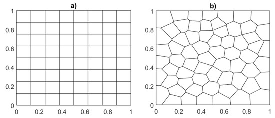
Figure 4. Sample polygonal meshes. (a) Uniform square mesh. (b) Regular Voronoi mesh.

By comparing the errors at two subsequent mesh refinements, we compute the convergence rate. From the theoretical results of Section 3, we expect optimal convergence rates $e_{h,0}^2=\mathcal{O}\left(h^{k+1}\right)$ and $e_{h,1}^2=\mathcal{O}\left(h^k\right)$, assuming that the exact solution is smooth enough.

Example 1

Consider the model problem given in Equation (7), with a nonlinear term, $f\left(u\right)=u(1-u)(u-1)$, $\mathit{x}=(x,y)$ and known load function given as

$$\begin{array}{cc}\hfill g(\mathit{x},t)=& \left(\Gamma (1+\alpha )+2{\pi }^2{t}^{\alpha }\right)\sin \left(\pi x\right)\sin \left(\pi y\right)+t^{\alpha }\sin \left(\pi x\right)\sin \left(\pi y\right)\hfill \\ \hfill & \left(2t^{\alpha }\sin \left(\pi x\right)\sin \left(\pi y\right)-{\left(t^{\alpha }\sin \left(\pi x\right)\sin \left(\pi y\right)\right)}^2-1\right).\hfill \end{array}$$

with $\Omega ={[0,1]}^2$ and $\partial \Omega =0$, which appropriately determines the impulse transport over a polygonal domain. These conditions ensure stability in the numerical approximation and provide a well-posed framework for solving the governing equation. To illustrate this, we present simulations of impulse transport over a polygonal domain. The results demonstrate the robustness of the numerical scheme, showing consistent convergence behavior and error estimates.

Figure 5 and Figure 6 show the VEM solutions and associated error plots for $\alpha =0.6$, computed on uniform square and regular Voronoi meshes, respectively, using first-order VEM ($k=1$). Similarly, Figure 7 and Figure 8 present the VEM solutions and error plots under identical conditions for the second-order VEM ($k=2$). These results have been obtained using the VEM formulation in (7).

Figure 5. Visualization of (a) VEM results and (b) error analysis for VEM order $k=1$ at $\alpha =0.6$ on uniform square meshes.

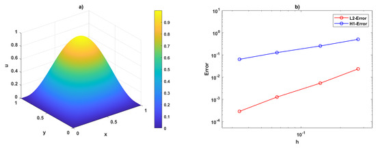
Figure 6. Visualization of (a) VEM results and (b) error analysis for VEM order $k=1$ at $\alpha =0.6$ on regular Voronoi meshes.

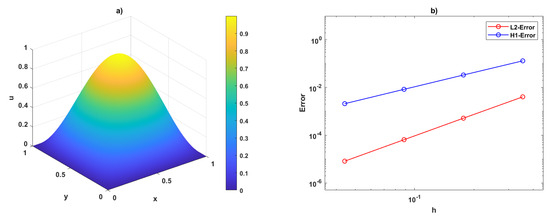
Figure 7. Visualization of (a) VEM results and (b) error analysis for VEM order $k=2$ at $\alpha =0.6$ on uniform square meshes.

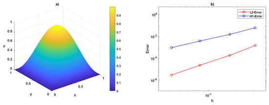
Figure 8. Visualization of (a) VEM results and (b) error analysis for VEM order $k=2$ at $\alpha =0.6$ on regular Voronoi meshes.

The computed results, including $L^2$-norm and $H^1$-norm errors alongside the rates of convergence (roc), are tabulated. Specifically:

• Table 1 and Table 2 provide the computed norms and rates of convergence with VEM order $k=1$ on uniform square meshes.
  Table 1. Data for $\alpha =0.3,0.6$ over uniform square meshes, the $L^2(\Omega )$-norm, and roc ($k=1$).

  		$\mathit{\alpha }=0.3$		$\mathit{\alpha }=0.6$
  h	DoF	${\mathit{L}}^{\mathbf{2}}$-Norm	Rate	${\mathit{L}}^{\mathbf{2}}$-Norm	Rate
  ${\displaystyle \frac{1}{2^2}}$	25	5.154952 × 10−2	–	5.153625 × 10−2	–
  ${\displaystyle \frac{1}{2^3}}$	81	1.224224 × 10−2	2.0741	1.222845 × 10−2	2.0753
  ${\displaystyle \frac{1}{2^4}}$	289	3.010066 × 10−3	2.0240	2.996480 × 10−3	2.0289
  ${\displaystyle \frac{1}{2^5}}$	1089	7.408137 × 10−4	2.0226	7.274806 × 10−4	2.0423

  Table 2. Data for $\alpha =0.3,0.6$ over uniform square meshes, the $H^1(\Omega )$-seminorm, and roc ($k=1$).

  		$\mathit{\alpha }=0.3$		$\mathit{\alpha }=0.6$
  h	DoF	${\mathit{H}}^{\mathbf{1}}$-Norm	Rate	${\mathbf{H}}^{\mathit{1}}$-Norm	Rate
  ${\displaystyle \frac{1}{2^2}}$	25	7.005321 × 10−1	–	7.005239 × 10−1	–
  ${\displaystyle \frac{1}{2^3}}$	81	3.543888 × 10−1	0.9831	3.543856 × 10−1	0.9831
  ${\displaystyle \frac{1}{2^4}}$	289	1.778421 × 10−1	0.9947	1.778407 × 10−1	0.9947
  ${\displaystyle \frac{1}{2^5}}$	1089	8.900554 × 10−2	0.9986	8.900493 × 10−2	0.9986

• Table 3 and Table 4 provide corresponding values for VEM with $k=2$ on uniform square meshes.
  Table 3. Data for $\alpha =0.3,0.6$ over uniform square meshes, the $L^2(\Omega )$-norm, and roc ($k=2$).

  		$\mathit{\alpha }=0.3$		$\mathit{\alpha }=0.6$
  h	DoF	${\mathit{L}}^{\mathbf{2}}$-Norm	Rate	${\mathit{L}}^{\mathbf{2}}$-Norm	Rate
  ${\displaystyle \frac{1}{2^2}}$	81	4.083755 × 10−3	–	4.083701 × 10−3	–
  ${\displaystyle \frac{1}{2^3}}$	289	5.196267 × 10−4	2.9743	5.195754 × 10−4	2.9754
  ${\displaystyle \frac{1}{2^4}}$	1089	6.529531 × 10−5	2.9924	6.522287 × 10−5	2.9939
  ${\displaystyle \frac{1}{2^5}}$	4225	8.613596 × 10−6	2.9223	8.199919 × 10−6	2.9917

  Table 4. Data for $\alpha =0.3,0.6$ over uniform square meshes, the $H^1(\Omega )$-seminorm, and roc ($k=2$).

  		$\mathit{\alpha }=0.3$		$\mathit{\alpha }=0.6$
  h	DoF	${\mathit{H}}^{\mathbf{1}}$-Norm	Rate	${\mathit{H}}^{\mathbf{1}}$-Norm	Rate
  ${\displaystyle \frac{1}{2^2}}$	81	1.319297 × 10−1	–	1.319295 × 10−1	–
  ${\displaystyle \frac{1}{2^3}}$	289	3.357831 × 10−2	1.9742	3.357831 × 10−2	1.9742
  ${\displaystyle \frac{1}{2^4}}$	1089	8.432059 × 10−3	1.9936	8.432053 × 10−3	1.9936
  ${\displaystyle \frac{1}{2^5}}$	4225	2.110393 × 10−3	1.9984	2.110361 × 10−3	1.9984

• Table 5 and Table 6 display the computed norms and roc for VEM with $k=1$ on regular Voronoi meshes.
  Table 5. Data for $\alpha =0.3,0.6$ over regular Voronoi meshes, the $L^2(\Omega )$-norm, and roc ($k=1$).

  		$\mathit{\alpha }=0.3$		$\mathit{\alpha }=0.6$
  h	DoF	${\mathit{L}}^{\mathbf{2}}$-Norm	Rate	${\mathit{L}}^{\mathbf{2}}$-Norm	Rate
  ${\displaystyle \frac{1}{2^2}}$	66	2.321432 × 10−2	–	2.319921 × 10−2	–
  ${\displaystyle \frac{1}{2^3}}$	256	5.294615 × 10−3	2.1324	5.281239 × 10−3	2.1351
  ${\displaystyle \frac{1}{2^4}}$	999	1.264779 × 10−3	2.0656	1.251974 × 10−3	2.0767
  ${\displaystyle \frac{1}{2^5}}$	3998	2.957565 × 10−4	2.0964	2.836264 × 10−4	2.1421

  Table 6. Data for $\alpha =0.3,0.6$ over regular Voronoi meshes, the $H^1(\Omega )$-seminorm, and roc ($k=1$).

  		$\mathit{\alpha }=0.3$		$\mathit{\alpha }=0.6$
  h	DoF	${\mathit{H}}^{\mathbf{1}}$-Norm	Rate	${\mathit{H}}^{\mathbf{1}}$-Norm	Rate
  ${\displaystyle \frac{1}{2^2}}$	66	5.001585 × 10−1	–	5.001548 × 10−1	–
  ${\displaystyle \frac{1}{2^3}}$	256	2.511504 × 10−1	0.9938	2.511499 × 10−1	0.9938
  ${\displaystyle \frac{1}{2^4}}$	999	1.260075 × 10−1	0.9950	1.260075 × 10−1	0.9950
  ${\displaystyle \frac{1}{2^5}}$	3998	6.293241 × 10−2	1.0016	6.293263 × 10−2	1.0016

• Table 7 and Table 8 present the results for VEM with $k=2$ on regular Voronoi meshes.
  Table 7. Data for $\alpha =0.3,0.6$ over regular Voronoi meshes, the $L^2(\Omega )$-norm, and roc ($k=2$).

  		$\mathit{\alpha }=0.3$		$\mathit{\alpha }=0.6$
  h	DoF	${\mathit{L}}^{\mathbf{2}}$-Norm	Rate	${\mathit{L}}^{\mathbf{2}}$-Norm	Rate
  ${\displaystyle \frac{1}{2^2}}$	195	1.434247 × 10−3	–	1.434028 × 10−3	–
  ${\displaystyle \frac{1}{2^3}}$	767	1.795089 × 10−4	2.9982	1.793635 × 10−4	2.9991
  ${\displaystyle \frac{1}{2^4}}$	2997	2.259150 × 10−5	2.9902	2.237516 × 10−5	3.0029
  ${\displaystyle \frac{1}{2^5}}$	11995	2.872416 × 10−6	2.9754	2.868341 × 10−6	2.9636

  Table 8. Data for $\alpha =0.3,0.6$ over regular Voronoi meshes, the $H^1(\Omega )$-seminorm, and roc ($k=2$).

  		$\mathit{\alpha }=0.3$		$\mathit{\alpha }=0.6$
  h	DoF	${\mathit{H}}^{\mathbf{1}}$-Norm	Rate	${\mathit{H}}^{\mathbf{1}}$-Norm	Rate
  ${\displaystyle \frac{1}{2^2}}$	195	6.064623 × 10−2	–	6.064618 × 10−2	–
  ${\displaystyle \frac{1}{2^3}}$	767	1.479368 × 10−2	2.0354	1.479367 × 10−2	2.0354
  ${\displaystyle \frac{1}{2^4}}$	2997	3.690532 × 10−3	2.0031	3.690514 × 10−3	2.0031
  ${\displaystyle \frac{1}{2^5}}$	11995	9.079729 × 10−4	2.0231	9.078992 × 10−4	2.0232

• Figure 9 illustrates the differences in computational efficiency between square and Voronoi meshes. The plot compares iteration count and CPU time, showing that a reduction in iterations leads to decreased computational cost, reflecting the solver’s efficiency across mesh types.
  

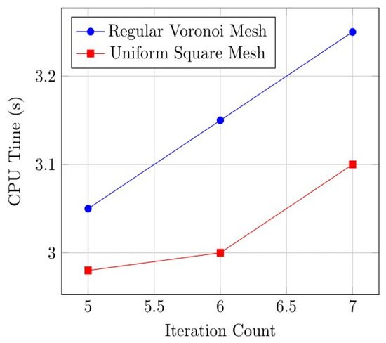  Figure 9. Computational efficiency and solver performance: uniform square vs. regular Voronoi mesh.

Additionally, Table 9 demonstrates that the discrete VEM scheme (7), for a fixed T, achieves a global temporal convergence rate of $\mathcal{O}\left(\tau \right)$. For this evaluation, the spatial mesh size is fixed at $h={10}^{-2}$ while refining $\tau$ to compute the error and temporal convergence. Figure 10 provides both the error plot and the reference convergence line.

Table 9. Error values and roc with fixed T for different values of $\alpha$ in time with regular Voronoi mesh configuration in spatial domain and fixed mesh size $h={10}^{-2}$.

		$\mathit{\alpha }=0.3$		$\mathit{\alpha }=0.6$
T	K	${\mathbf{L}}^{\mathbf{2}}$-Norm	Rate	${\mathbf{L}}^{\mathbf{2}}$-Norm	Rate
1	20	1.265 × 10−3	–	1.252 × 10−3	–
	25	1.019 × 10−3	0.95	1.012 × 10−3	0.95
	30	8.561 × 10−4	0.96	8.431 × 10−4	1.00
	35	7.354 × 10−4	0.98	7.121 × 10−4	1.10
0.1	20	1.652 × 10−3	–	1.681 × 10−3	–
	25	1.313 × 10−3	1.03	1.320 × 10−3	1.08
	30	1.081 × 10−3	1.07	1.090 × 10−3	1.05
	35	9.012 × 10−4	1.18	9.132 × 10−4	1.15

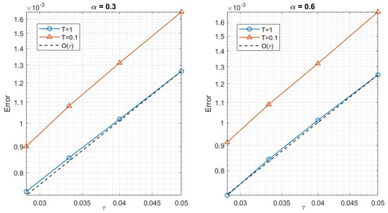
Figure 10. Error and convergence plots in temporal direction at different $\alpha$ values and different T values.

6. Conclusions

In this study, we have developed and analyzed a numerical scheme for approximating impulse transport modeled by a nonlinear time-fractional partial differential equation with Dirichlet boundary conditions. We presented the model formulation, proposed a virtual element method for its spatial discretization, and introduced a fully discrete time-stepping scheme. Theoretical convergence analysis was performed in both the $L^2$-norm and $H^1$-seminorm, and the results were confirmed through extensive numerical experiments. Fractional-order models are widely applicable in various scientific and engineering contexts, especially for systems with memory and hereditary properties. Consequently, efficient numerical techniques like VEM are essential to approximate such models accurately on general polygonal meshes.

Our primary objective was to assess the efficiency, stability, and accuracy of the proposed scheme, rather than to validate the physical accuracy of the model equation itself. Nevertheless, the mathematical framework provided offers insights into potential real-world applications. While the design and formulation of the model equation are briefly introduced, this serves to provide readers with insights into its structure and applicability rather than as a comparative evaluation against existing models.

Our analysis suggests that this modeling approach can be beneficial in the context of sensory prosthetics. Furthermore, the immediate emphasis of our research is to examine neurodegenerative diseases in relation to impulse transport and to illustrate how these disorders affect impulse transmission and vice versa.

References

- Podlubny, I. (Ed.) Fractional Differential Equations: An Introduction to Fractional Derivatives, Fractional Differential Equations, to Methods of Their Solution and Some of Their Applications; Elsevier: Amsterdam, The Netherlands, 1999; Volume 198. [Google Scholar]
- Wazwaz, A.M. Linear and Nonlinear Integral Equations: Methods and Applications, 1st ed.; Springer Publishing Company, Incorporated: Berlin/Heidelberg, Germany, 2011. [Google Scholar]
- Kilbas, A.A.; Srivastava, H.M.; Trujillo, J.J.E. Theory and Applications of Fractional Differential Equations; North-Holland Mathematics Studies; Elsevier: Amsterdam, The Netherlands, 2006; Volume 204. [Google Scholar]
- Baeumer, B.; Kov’acs, M.; Sankaranarayanan, H. Higher order Grünwald approximations of fractional derivatives and fractional powers of operators. Trans. Am. Math. Soc. 2014, 367, 813–834. [Google Scholar] [CrossRef]
- Sousa, E. Finite difference approximations for a fractional advection diffusion problem. J. Comput. Phys. 2009, 228, 4038–4054. [Google Scholar] [CrossRef]
- Acosta, G.; Borthagaray, J. A Fractional Laplace Equation: Regularity of Solutions and Finite Element Approximations. SIAM J. Numer. Anal. 2015, 55. [Google Scholar] [CrossRef]
- Acosta, G.; Bersetche, F.; Borthagaray, J. A short FE implementation for a 2d homogeneous Dirichlet problem of a Fractional Laplacian. Comput. Math. Appl. 2017, 74, 784–816. [Google Scholar] [CrossRef]
- Ervin, V.; Roop, J. Variational formulation for the stationary fractional advection dispersion equation. Numer. Methods Partial Differ. Equ. 2006, 22, 558–576. [Google Scholar] [CrossRef]
- Esen, A.; Ucar, Y.; Yagmurlu, N.; Tasbozan, O. A Galerkin Finite Element Method to Solve Fractional Diffusion and Fractional Diffusion-Wave Equations. Math. Model. Anal. 2013, 18, 260–273. [Google Scholar] [CrossRef]
- Jin, B.; Lazarov, R.; Zhou, Z. A Petrov-Galerkin Finite Element Method for Fractional Convection-Diffusion Equations. SIAM J. Numer. Anal. 2015, 54, 481–503. [Google Scholar] [CrossRef]
- Zhang, X.; Wei, L.; Liu, J. Application of the LDG method using generalized alternating numerical flux to the fourth-order time-fractional sub-diffusion model. Appl. Math. Lett. 2025, 168, 109580. [Google Scholar] [CrossRef]
- Luo, W.H.; Huang, T.Z.; Wu, G.C.; Gu, X.M. Quadratic spline collocation method for the time fractional subdiffusion equation. Appl. Math. Comput. 2016, 276, 252–265. [Google Scholar] [CrossRef]
- Zhao, Y.L.; Gu, X.M.; Ostermann, A. A Preconditioning Technique for an All-at-once System from Volterra Subdiffusion Equations with Graded Time Steps. J. Sci. Comput. 2021, 88, 11. [Google Scholar] [CrossRef]
- Gu, X.M.; Wu, S.L. A parallel-in-time iterative algorithm for Volterra partial integro-differential problems with weakly singular kernel. J. Comput. Phys. 2020, 417, 109576. [Google Scholar] [CrossRef]
- Beirão da Veiga, L.; Brezzi, F.; Cangiani, A.; Manzini, G.; Marini, L.D.; Russo, A. Basic principles of Virtual Element Methods. Math. Model. Methods Appl. Sci. 2012, 23. [Google Scholar] [CrossRef]
- Ahmad, B.; Alsaedi, A.; Brezzi, F.; Marini, L.D.; Russo, A. Equivalent projectors for virtual element methods. Comput. Math. Appl. 2013, 66, 376–391. [Google Scholar] [CrossRef]
- Adak, D.; Natarajan, S. Virtual element method for semilinear sine–Gordon equation over polygonal mesh using product approximation technique. Math. Comput. Simul. 2020, 172, 224–243. [Google Scholar] [CrossRef]
- Arrutselvi, M.; Natarajan, E. Virtual element method for nonlinear convection–diffusion–reaction equation on polygonal meshes. Int. J. Comput. Math. 2020, 98, 1852–1876. [Google Scholar] [CrossRef]
- Beirão da Veiga, L.; Lovadina, C.; Vacca, G. Divergence free virtual elements for the stokes problem on polygonal meshes. ESAIM: Math. Model. Numer. Anal. 2017, 51, 509–535. [Google Scholar] [CrossRef]
- Beirão da Veiga, L.; Brezzi, F.; Marini, L.D.; Russo, A. Mixed Virtual Element Methods for general second order elliptic problems on polygonal meshes. ESAIM Math. Model. Numer. Anal. 2014, 50, 727–747. [Google Scholar] [CrossRef]
- Antonietti, P.F.; Manzini, G.; Verani, M. The conforming virtual element method for polyharmonic problems. Comput. Math. Appl. 2020, 79, 2021–2034. [Google Scholar] [CrossRef]
- Antonietti, P.; Beirão da Veiga, L.; Manzini, G. (Eds.) The Virtual Element Method and Its Applications; SEMA SIMAI Springer Series; Springer: Berlin/Heidelberg, Germany, 2022; Volume 31. [Google Scholar]
- Dar, Z.M.; Arrutselvi, M.; Chandru, M.; Manzini, G.; Natarajan, S. Analytical and Numerical Methods for Solving Fractional-Order Partial Differential Equations and the Virtual Element Method. SSRN 2024. [Google Scholar] [CrossRef]
- Li, D.; Liao, H.l.; Sun, W.; Wang, J.; Zhang, J. Analysis of L1-Galerkin FEMs for Time-Fractional Nonlinear Parabolic Problems. Commun. Comput. Phys. 2018, 24, 86–103. [Google Scholar] [CrossRef]
- Li, D.; Zhang, J. Efficient implementation to numerically solve the nonlinear time fractional parabolic problems on unbounded spatial domain. J. Comput. Phys. 2016, 322, 415–428. [Google Scholar] [CrossRef]
- Zhang, Y.; Feng, M. A local projection stabilization virtual element method for the time-fractional Burgers equation with high Reynolds numbers. Appl. Math. Comput. 2023, 436, 127509. [Google Scholar] [CrossRef]
- Dar, Z.M.; Chandru, M. A virtual element scheme for the time-fractional parabolic PDEs over distorted polygonal meshes. Alex. Eng. J. 2024, 106, 611–619. [Google Scholar] [CrossRef]
- Dar, Z.M.; Arrutselvi, M.; Muthusamy, C.; Natarajan, S.; Manzini, G. Virtual element approximations of the time-fractional nonlinear convection-diffusion equation on polygonal meshes. Math. Eng. 2025, 7, 96–129. [Google Scholar] [CrossRef]
- Metzler, R.; Jeon, J.H.; Cherstvy, A.G.; Barkai, E. Anomalous diffusion models and their properties: Non-stationarity, non-ergodicity, and ageing at the centenary of single particle tracking. Phys. Chem. Chem. Phys. 2014, 16, 24128–24164. [Google Scholar] [CrossRef]
- Jin, B.; Li, B.; Zhou, Z. Numerical Analysis of Nonlinear Subdiffusion Equations. SIAM J. Numer. Anal. 2018, 56, 1–23. [Google Scholar] [CrossRef]
- Mascotto, L. Ill-conditioning in the virtual element method: Stabilizations and bases. Numer. Methods Partial Differerential Equ. 2018, 34, 1258–1281. [Google Scholar] [CrossRef]
- Kumar, D.; Chaudhary, S.; Srinivas Kumar, V. Fractional Crank–Nicolson–Galerkin finite element scheme for the time-fractional nonlinear diffusion equation. Numer. Methods Partial Differ. Equ. 2019, 35, 2056–2075. [Google Scholar] [CrossRef]
- Jin, B.; Li, B.; Zhou, Z. An analysis of the Crank-Nicolson method for subdiffusion. IMA J. Numer. Anal. 2017, in press. [Google Scholar] [CrossRef]
- Dimitrov, Y. Numerical approximations for fractional differential equations. J. Fract. Calc. Appl. 2015, 5, 1–45. [Google Scholar]
- Thomée, V. Galerkin Finite Element Method for Parabolic Problems; Springer: Berlin/Heidelberg, Germany, 2006; Volume 1054. [Google Scholar] [CrossRef]
- Chen, H.; Holland, F.; Stynes, M. An analysis of the Grünwald–Letnikov scheme for initial-value problems with weakly singular solutions. Appl. Numer. Math. 2019, 139, 52–61. [Google Scholar] [CrossRef]
- Gorenflo, R.; Kilbas, A.A.; Mainardi, F.; Rogosin, S.V. Mittag–Leffler Functions, Related Topics and Applications; Springer: Berlin/Heidelberg, Germany, 2016. [Google Scholar]
- Cangiani, A.; Manzini, G.; Sutton, O.J. Conforming and nonconforming virtual element methods for elliptic problems. IMA J. Numer. Anal. 2016, 37, 1317–1354. [Google Scholar] [CrossRef]
Disclaimer/Publisher’s Note: The statements, opinions and data contained in all publications are solely those of the individual author(s) and contributor(s) and not of MDPI and/or the editor(s). MDPI and/or the editor(s) disclaim responsibility for any injury to people or property resulting from any ideas, methods, instructions or products referred to in the content. |
© 2025 by the authors. Licensee MDPI, Basel, Switzerland. This article is an open access article distributed under the terms and conditions of the Creative Commons Attribution (CC BY) license (https://creativecommons.org/licenses/by/4.0/).